行政院國家科學委員會專題研究計畫 成果報告
銀行產業特性、品質因素與生產力及效率衡量(2/2)
計畫類別: 整合型計畫 計畫編號: NSC93-2415-H-009-013- 執行期間: 93 年 08 月 01 日至 94 年 07 月 31 日 執行單位: 國立交通大學資訊與財金管理學系 計畫主持人: 黃台心 計畫參與人員: 廖盈婷 報告類型: 完整報告 處理方式: 本計畫可公開查詢中 華 民 國 94 年 9 月 26 日
An Examination on the Cost Efficiency of Banking Industry under Multiple Output Prices’ Uncertainty
By
Tai-Hsin Huang Professor
Correspondence Author: E-mail: [email protected] and [email protected] Department of Information and Finance Management
National Chiao Tung University 1001 Ta Hsueh Road, Hsinchu Taiwan 300, The Republic of China
And
Ying-Ting Liao
Master
Graduate Institute of Economics Tamkang University Tamsui, Taipei Hsien
An Examination on the Cost Efficiency of Banking Industry under Multiple Output Prices’ Uncertainty
Abstract
This paper formulates a behavioral model of profit maximization, which explicitly incorporates both multiple output prices’ risk and safety-first practice. This theoretical model is specifically suitable for investigating financial institutions, whose output prices frequently encounter a variety of risks, such as loan default/arrears. The sample banks are empirically found to be highly risk-averse. Furthermore, risk preferences exert little effect on the technical efficiency estimates, whereas the same estimates obtained by the standard fixed-effect model under certainty tend to be overestimated. Evidence is found that a specialized bank offering a single product with a larger scale of production will be preferable, when an uncertain atmosphere is pervasive.
JEL Classification: C33 D81 G21
Keywords: output prices’ uncertainty safety-first risk premium scale economies technical efficiency
An Examination on the Cost Efficiency of Banking Industry under Multiple Output Prices’ Uncertainty
For the past few decades, many researchers have been devoted to developing various theoretical models from different angles to explain the responses of outputs and input demands to risk attitudes and changes in risk. See, for example, Sandmo (1971), Ishii (1978), Hartman (1975, 1976), Batra and Ullah (1974), Holthausen (1976), Smith (1970), Turnovsky (1973), Chambers (1983), Appelbaum and Katz (1986), Dalal (1990), and Viaene and Zilcha (1998), among others. The most common assumption in the literature is that producers maximize a von-Neumann-Morgenstern utility function in a competitive market. While there exist versatile analytic theories having been developed to understand the effects of uncertainty on firm behavior, relatively few empirical exercises utilize these frameworks, except for Parkin (1970), Just (1974), Antonovitz and Roe (1986), Appelbaum (1991), Appelbaum and Kohli (1993), Appelbaum and Ullah (1997), Roosen and Hennessy (2003), Wolak and Kolstad (1991), Ballivian and Sickles (1994), Hughes and Mester (1998), and Huang and Fu (2001).1
The purpose of this article is twofold. First, it is intended as a systematic study of the risk-averse behavior under multiple output prices’ uncertainty for competitive banks. A specific attitude toward risk - safety first - which was initiated by Roy (1952) and later by Telser (1955) is postulated by the theoretical model.2 The noticeable feature of the current study lies in its improvement over the previous works that dealt with single output price uncertainty. The uncertainty might come from the volatility of the bank’s investment returns and the risk of loan defaults. Investments and loans are two outputs defined by the intermediation approach in the literature of banking productivity and efficiency.
Second, given that there are relatively few empirical applications to firm behavior under uncertainty, this paper proposes an empirically feasible framework for analyzing such a behavior. Assuming multiple output prices’ uncertainty and rational expectations, we develop an estimable model which can be used to identify firms’ attitudes toward risk directly and to explain the impact of the price uncertainty and risk aversion on producers’ decision making. More specifically, we utilize the
1
In the context of risk-reducing inputs, proposed by Just and Pope (1978) under production uncertainty, several empirical studies have emerged recently; for example, Kumbhakar (1993), Battese et al. (1997), and Tveteras (1999). These papers unanimously investigate agricultural data, possibly pervasive of production risk.
2
parameter estimates to calculate scale and product mix economies of banks with and without regard to price uncertainty and to identify the influence of risk attitudes on the economies of scale and scope.
As an exemplification, we investigate the risk-averse behavior and safety-first practice of bank management facing uncertainty at the firm level of individual banks in Taiwan, for the period of 1996 to 2002. This particular sample is chosen due to the fact that it covers a turbulent time period with some regulatory changes and several changes in market conditions. It is known that the 1997 Asian financial crisis overwhelmed many economies in Northeast and Southeast Asia, including Taiwan. In contrast to those of other Asian countries, Taiwan weathered the storm very well. Both its stock and exchange markets turned out to be relatively stable.3 Some factors were likely to be responsible for its exemplary performance. Among them, deregulation starting from 1989 and more conservative risk management in the banking industry may have contributed to the smoothness of the financial sector. Somewhat later, the island did experience an economic downturn, in 2001. The unemployment rate rose from 3% in 2000 to 4.6% in 2001, and further increased to 5.2% in 2002. In fact the theoretical model developed by this article can be directly applied to other industries, characterized by multiple output prices’ risk, in various countries.
The rest of the paper is organized as follows. Section 2 develops a theoretical model of firm behavior under multiple output prices’ uncertainty. Section 3 addresses an econometric model. Section 4 briefly introduces the sample, while Section 5 analyzes the empirical results. Section 6 concludes the paper.
2. Theoretical Framework
Suppose a competitive firm hires m variable inputs, denoted by , to produce, for expository convenience and without loss of
generality, two outputs, as denoted by
(
1, , mX = X ! X
)
′)
(
1, 2Y = Y Y ′. Later, Y will be defined as
the amount of investments and Y is the amount of loans. The model to be developed below can be easily extended to the case of outputs. Vectors X and Y are both non-negative. The corresponding vectors of input and output prices are
1 2 2 n> 3
Between the second quarter of 1997 and the first quarter of 1998, the value of the currencies in Thailand, Indonesia, South Korea, Malaysia, and the Philippines dropped substantially, ranging from 57.46% to 228.95%, and their stock markets also fell, to a scope of 26.59% to 50.89%. During the same period, the value of Taiwan’s currency decreased 21.79%, while its stock market index declined 13.24%.
(
1, , m)
W = W ! W ′ and P=
(
P P1, 2)
′, respectively. Since the output prices are stochastic due possibly to the volatile banks’ investment returns and the risk of loan defaults, we assume j j P =P j P j P vj j v + , j=1, 2, (2.1)where is the mean value of the jth output price and is the statistical noise with
mean 0 and constant covariance
j v 1 11 12 22 2 ( ) v Cov v Cov v σ σ σ = = .
Both and are unobservable. The mean vector of the random prices is equal
to 1 2 ( ) P E P P P = = , and its covariance matrix is the same as Cov v( ).
It is noteworthy that the above model specification is substantially different from Huang and Fu (2001) in two aspects. First, they presumed an aggregated single output quantity index Y and the corresponding single output price index P, instead of original multiple outputs and prices. Second, they specified a multiplicative form of the random output price as P=Pev , where e denotes the natural exponent. Although this specification has its own merit, it appears to be difficult to find a suitable distribution for disturbance v with E e( )v = .1 4
The random profit function is expressed as
P Y′ W X′
Π = − . (2.2)
Since P is naturally restricted to be non-negative, so is P . This implies that, once X has been elected, the firm’s (expected) maximum economic loss is −W X′ . It can be shown that ( ) E Π = Π =P Y′ −W X′ , (2.3) and 4
The random component e is usually assumed to be distributed as a lognormal. However, the mean of will imply that the variance of has to be zero, which is implausible.
v
( )v 1
2 2 2
1 11 2 22 1 2 12
( ) 2
Var Π =σ =Y σ +Y σ + Y Yσ . (2.4)
In the literature it is conventionally assumed that the firm’s behavior under uncertainty is to maximize the expected utility of profits, E U[ ( )]Π , where E is the expectations operator and is a von-Neumann-Morgenstern utility function with
and U
( ) U • ( ) 0
U ′ Π > ′′ Π < . Thus, the firm is assumed to be risk averse. We argue ( ) 0 that the managers’ and/or stockholders’ goals may not simply pursue the maximization of the expected utility of profits, even though both prefer a higher level of expected utility. This seems to be meaningful, particularly in the banking sector, where risky investments and loans usually yield higher expected returns, but are frequently accompanied by considerable variability and risk, which may give rise to bank failure.
Following Huang and Fu (2001), banks’ managers are instead aware of a threshold utility level such that the probability of the utility of the random profit being less than or equal to falls short of , a subjective acceptable probability and likely to be firm specific. The threshold utility U reflects a critical level, below which either bank suffers insolvency, or the firing of the managers will result. The best interest of managers and/or stockholders is formulated as the maximization of the expected utility subject to the subjective probability, . This attitude toward risk is referred to as safety first, pioneered by Roy (1952) when dealing with a theory of asset holding, and followed by Telser (1955) who introduced the theory of hedging.
* U * U T* * * * ProbU( )Π ≤U T≤
The safety-first principle can be reformulated as maximizing the threshold utility subject to the same probability constraint, as suggested by Kataoka (1963). Mathematically, a firm’s behavior is assumed to
*
U
Max. U*
s.t. ProbU
( )
Π ≤U*=ProbU P Y(
′ −W X′)
≤U*≤T . (2.5) * This new maximization problem is perhaps easier to solve, because the objectivefunction is now a truncation point of the probability distribution of utility levels. Substituting equation (2.1) into (2.5) and taking the inverse function of , the probability constraint can be rewritten as
( ) U •
(
)
* 1 1 2 2 1( )
* Prob U P Y W X U Prob Y v Y v U U σ σ − + − Π ′ ′ − ≤ = ≤ ( )
1 * * U U T σ − − Π = Φ ≤ , (2.6)where denotes the cumulative distribution function (cdf) of the standard normal and is the inverse utility function.
( ) Φ• 1 ( ) − • U
Taking the inverse function of the cdf of the standard normal on both sides of (2.6), the probability constraint is restated as
( )
( )
1 * 1 *
U− U ≤P Y′ −W X′ + Φ− T σ. (2.7)
According to microeconomic theory, the utility function and the inverse utility function are both monotonic. This indicates that the maximization of the threshold utility level U subject to the probability constraint is equivalent to the unconstrained maximization of the threshold profit
*
( )
* 1 U− U Π = * in (2.7), i.e., Max. Π =* P Y′ −W X′ −R Y Y( , )1 2 , (2.8) where R Y Y( , )1 2 1(T*)σ −= −Φ defines the risk premium arising from uncertainty. This represents the difference between the expected profit under uncertainty and the profit under certainty, which leaves managers indifferent between the two choices. The corresponding maximum threshold utility is given by
[
]
*
1 2
( ) ( ) ( , )
U Π =U E Π −R Y Y . (2.9)
It is readily seen that model (2.8) can be reduced to the standard certainty case by letting σ11=σ22 =σ12 = , i.e., by removing the assumption of output price 0 uncertainty.
The risk premium contains important economic implications. Its value can be positive, zero, or negative, provided that the decision makers are risk-averse, risk-neutral, or risk-loving. The size of the risk premium at the firm level relies crucially on three factors. First, it depends on the degree of risk-aversion,
It is reflected by the underlying subjective probability measure, , such that 1 * (T ) −Φ− . = ) * T
(
)
1( )
* * 1 2 risk-averse , 0 risk-neutral 0 0.5 risk-loving R Y Y − T T > < < = ⇒ Φ = ⇒ < > > .is, the more risk-averse the decision maker is. Second, it is affected by the level of risk arising from the joint probability distribution of the two output prices. Finally, it depends on the level of the two outputs. Therefore, risk premiums increase as either risk aversion increases, or the level of risk increases, or the level of outputs increases, or any combinations of them occur together. As shown by equation (2.8), risk premiums represent extra costs for the risk-averse bank that influence its optimal organization.
Because higher costs decrease economic well-being, actions that lower risk aversion and risk level will lower risk premiums and thus diminish the costs of a bank’s operation. As a result, these actions will ultimately benefit the economy as a whole by improving economic efficiency as well as increasing the utility of profits. On the basis of equation (2.8), the lower the risk premium is, the higher the maximum attainable profits will be, and so the greater utility acquired, other things being constant. The enhancement of economic efficiency will be discussed after obtaining the first-order conditions of the profit maximization.
The magnitude of R• depends on endogenous variables ( ) and Y . Larger enterprises have greater estimates of the risk premiums. To get a more concrete idea about the relative scale of
1
Y 2
( )
R• , we further define and calculate the rate of the risk premium (RRP) as the ratio of the risk premium to the expected total revenue, i.e.,
1 2 1 1 2 2 ( , ) R Y Y RRP PY P Y = + . (2.10)
The RRP measure tells us the relative importance that the risk attitudes play in the process of decision-making.
To solve for the optimal outputs under uncertainty, we adopt the two-step procedure on the basis of microeconomic theory. A cost function, C W , is first derived by the minimization of the firm’s expenditure on employing variable inputs subject to a given production possibilities set. It is then plugged into equation (2.8) and the choice variables become Y and . The first-order necessary conditions for a maximum are then expressed as
* ( ′ ′,Y ) 1 Y1 * * * 1 1 1 1 0 C MR Y Y ∂Π ∂ Π = = − = ∂ ∂ , (2.11) and * * * 2 2 2 2 0 C MR Y Y ∂Π ∂ Π = = − = ∂ ∂ , (2.12)
( )
(
1 * 1
1 1 11
MRP = Φ− T σ− Yσ +Y2σ12
)
signifies the marginal risk premium of Y , caused by producing an additional unit of .1 1 Y 2 = 2+ 2 Y MRP = Φ−
)
σ− 2 * j C Y ∂ ∂ j=1, 2 * * * j j j P = ∂C ∂Y =C j=1, 2 ( RLikewise we can see that MR P MRP denotes the expected marginal
revenue of , in which 2 1
(
T* 1(
Y2σ22 +Yσ)
represents the marginal risk premium of Y , arising from producing an additional unit of Y . Finally, 2, , is the standard marginal cost function of output j.
2
1 12
Equations (2.11) and (2.12) incorporate the optimality conditions adaptable for uncertainty where the firm’s expected marginal revenue equals marginal cost. Due to the presence of uncertain output prices, the expected marginal revenue deviates from the expected output price to an extent determined by the marginal risk premium.
An interesting question is often raised by the introduction of the uncertainty: do the optimal outputs differ from the well-established competitive solution under certainty? Using our notation, the solution under certainty is characterized by , , i.e., the equality between respective output prices and marginal costs. For a single output case, it is evident from equation (2.11) that as long as the marginal cost is positive, the output level satisfying the first-order condition of a risk-averse firm will be less than the optimal level of output under certainty. This result is similar to, for example, Sandmo (1971), Appelbaum (1991), and Robison and Barry (1987). However, things become more complicated for multiple output situations. We shall come back to this issue shortly.
Whether or not the sufficient condition can be held falls in the range of empirical aspects and will be answered by the empirical study section later. From a theoretical point of view, the existence of • and its resultant ) MRP , 1, j j= 2, deviates the optimal solutions from the standard competitive equilibrium, irrespective of bank managers’ risk attitudes. Analogous to imperfect competition, this gives rise to the distortion of resource allocation, leaving room for promoting economic efficiency.
As for the second-order conditions for a profit maximum, the following shows what is needed: * * 1 11 11 11 1 0 MR C Y ∂Π Π = = − ≤ ∂ * , (2.13)
* * 2 22 22 22 2 0 MR C Y ∂Π Π = = − ≤ ∂ * * , (2.14) * * 12 21 MR12 C12 Π = Π = − , (2.15) and * * *2 11 22 12 0 ∆ = Π Π − Π ≥ , (2.16) where MR11= ∂MR1 ∂Y , 1 MR22 = ∂MR2 ∂Y2 , MR12 = ∂MR1 ∂ , Y2 C11* = ∂C1* ∂Y , 1
* *
22 2 2
C C
∂ = ∂ ∂Y , and * * *
12 = 21 = ∂C1 ∂Y2
C C . It can readily be shown that these
second-order conditions will guarantee the supply functions of Y and go upward sloping with respect to expected own output prices, consistent with the standard results under certainty and with the case of a risk-averse firm. See, for example, Sandmo (1971), Appelbaum and Katz (1986), and Appelbaum and Ullah (1997). A detailed derivation on equations (2.13) to (2.16) and the proofs for a positive association between quantities supplied and the expected own prices are shown in Appendix 1.
1 Y2
By reference to equations (A9) to (A11) of Appendix 1, since the presence of uncertain output price P1 alone will lower the expected marginal revenue
1 1 ( )
P +MRP ≤P
* 12
C
1 , it is anticipated that the optimal level of production for will
definitely decrease, whereas the effect on optimal is ambiguous, depending on the sign of . 1 Y 2 Y 5
The reverse is true when alone is subject to uncertainty. If both output prices are subject to uncertainty and cause the expected marginal revenues to change by an equal amount, i.e.,
2
P
1 2
dP =dP ≠ 0, then the effects on the optimal productions of and Y are both indeterminate, as shown by equations (A12) and (A13). A salient feature of the model worth mentioning is that once the unknown technology and risk parameters are empirically estimated, conditions (2.13) to (2.16) and (A9) to (A13) can be checked for each observation. Furthermore, the effects of
1
Y 2
1 2
dP =dP ≠ 0 on the optimal production of both outputs can be evaluated. 3. Empirical Specifications
5
Note that term MRP1 is now equal to Φ−1(T Y*) 1−1σ11−1 / 2 ≤ and equation (A4) reduces to 0 . 12 Π * 12 C = −
In this section we deduce a non-linear simultaneous equation system in the first subsection, followed by the definitions of scale and scope economies.
3.1 Regression Equations
Substituting equation (2.1) into (2.11) and (2.12) and rearranging terms, we transform equation (2.1) into econometric specifications:
* 1 * 1 1 1 11 1 ( ) ( ) it it it it it it C P T Y Y Y σ σ σ − − ∂ = − Φ + + ∂ 2 12 v , (3.1) 1 and * 1 * 1 2 2 22 2 ( ) ( ) it it it it it it C P T Y Y Y σ σ σ − − ∂ = − Φ + + ∂ 1 12 v2 n T , (3.2) where subscript i ( 1, , )= … indexes firms and t ( 1, , )= … indexes time.
The unobserved expected output prices Pj
P
have been successfully replaced by equivalent observable counterparts. Equations (3.1) and (3.2) are regression equations with dependent variables and , while explanatory variables , , and input prices are embedded in the cost function C and the marginal risk premiums. All the regressands and regressors are observable. However, these regression equations are not estimable, unless the functional forms of the two marginal costs are specified a priori.
1
P 2 Y1 Y2
*
The translog cost function is widely used by numerous empirical researchers, which is a second-order approximation to a twice-differentiable arbitrary cost function. In line with the convention, we specify such a function that also accounts for input-oriented technical efficiency (TE) level, ui, as
* 3 lnCit =lnCit+ +ui vit 2 3 2 2 0 1 1 1 1 1 ln ln ln ln 2 j j k k jm j j k j m Y W Y α α β α = = = = = +
∑
+∑
+∑∑
Ym 3 3 2 3 3 1 1 1 1 1 ln ln ln ln 2 k m km k m j k jk j k i it W W Y W u v β γ = = = = +∑∑
+∑∑
+ + , (3.3)where denotes the observed total expenditures of firm i at time t. Some standard regularity conditions can be imposed directly on the cost function, which include (i) linear homogeneity
it C 3 1 1 k k β = =
∑
, 3 1 0 km m β = =∑
, k =1, 2, 3, 3 1 0, 1, 2, jk k j γ = = =∑
and (ii) symmetry , , 1, 2, 3, km mk k m β =β ∀ = , , 1, 2. jm mj j m α =α ∀ =
There are ten restrictions that should be imposed during an estimation. Other regularity conditions, such as negative semi-definiteness, can be checked after estimating the cost function. Notation represents the incremental (log) cost due to the presence of the input-oriented technical inefficiency, which will be regarded as the firm-specific fixed-effect later. Variable is the random disturbance required by regression equations.
i
u
3it
v
Given that we have the translog cost function (3.3), the marginal cost functions of and can be derived straightforward. The structural coefficients of equations (3.1) through (3.3) can now be estimated simultaneously by the full information maximum likelihood (FIML) method.
1 Y Y 2 Y 6
This system method is particularly suitable for non-linear simultaneous equations like the one here, since the second moments of the stochastic disturbances and emerge in the structural equations (3.1) and (3.2). Its estimators are shown to be consistent, asymptotically efficient, and their asymptotic distribution is normal. Notice that the proposed estimation procedure in effect amounts to estimating a profit function, because it involves both the revenue and cost side of bank operations. Moreover, the marginal cost functions derived by differentiating the translog cost function with respect to and have to be substituted into equations (3.1) and (3.2), thus allowing for the risk preferences and risk parameters to be consistent with profit maximization and the constraints on outputs imposed by the technology, i.e., the cost function.
1
v v2
1
Y
2
Assuming that random vector V =( )v1 v v '2 3 is distributed as a multivariate normal, it is not difficult to derive the log-likelihood function for equations (3.1) to (3.3). Therefore, it is ignored.
3.2 Scale and Scope Economies
Two types of measure are going to be calculated. (1) Overall scale economies (OSE):
* 2 * 1 ( ', ') ( ', ') i i i C W Y OSE Y C W Y = =
∑
. (3.4)Returns to scale are increasing, constant, or decreasing, as OSE is greater than,
6
In fact, two out of the three cost share equations, implied by the translog cost function, can also be estimated simultaneously in order to improve the accuracy of the estimates. Unfortunately, this implies that all inefficiencies are technical in essence, excluding the possibility of allocative inefficiency. See Berger (1993).
equal to, or less than unity. (2) Economies of Scope (SC):
Following Kim (1986), Mester (1996), and Huang and Wang (2004), scope economies are defined as
* * 1 1 2 1 2 2 * ( , , ') ( , , ') ( ', ') ( ', ') C Y W C Y W C Y W SC C W Y δ δ δ δ − + − − = * , (3.5)
where δj, equals to 10% of the sample minimum of Y , . Scope economies or diseconomies are present if SC exceeds or falls short of zero.
1, 2,
j= j j= 1, 2
4. Data Description
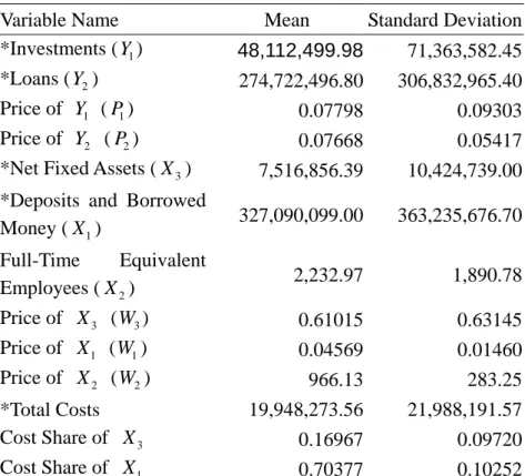
Following the intermediation approach, the current paper identifies two outputs and three inputs, extracted from the data bank of Taiwan Economic Journal. The sample period covers 1996 to 2002. Since some banks started their businesses after 1996, this unbalanced panel data set contains 49 commercial banks with sample size 324.7 The output entities are composed of investments ( ), which include government and corporate securities and stocks, and various short- and long-term loans (Y ). All kinds of deposits and borrowed money (
1
Y
2 X ), the number of full-time 1
equivalent employees (X ), and fixed assets net of depreciation (2 X ) are categorized 3 as inputs. Sample statistics of all variables are summarized in Table 4-1.
[Insert Table 4-1 Here]
Table 4-1 reflects that output item is the main product of the sample banks, which is more than five times as much as output Y on average. In practice, a bank’s excess reserves are often used to make loans with distinct terms of maturity. The remaining reserves will be used to buy securities and stocks. It is evident that the sample banks earn profits through the process of transforming funds (
2
Y
1
1
X ) into investments ( Y ) and loans (Y ) due to the discrepancy among the prices of 1 2 X , 1 , and . Input
1
Y
2
Y X appears to be the most important factor of production, because 1 its average cost share is as high as 70%.
5. Empirical Results
This section first presents the parameter estimates of three econometric models. Subsection 5.2 computes the risk premiums. Subsection 5.3 analyzes the implications of TE estimates, while the last subsection calculates scale and scope economies and various elasticities of substitution.
5.1 Parameter Estimates
7
At the end of 2002, there were 53 domestic banks in Taiwan. We preclude the two industrial banks and two specialized banks from the sample, since their activities differ dramatically from commercial banks.
Since is a probability measure dependent upon the managers’ attitudes toward risk, it is not directly observable, but is estimable after parameterization. There are several alternative ways of doing so. We choose to associate the subjective probability with a linear trend as:
*
T
*
0 1
T =a + t , a t=0, 1, , 6,… (5.1)
where t denotes the linear trend equaling the sample year minus 1996 (the first year of the panel data) and and a are unknown parameters, in which reflects the marginal change of the subjective probability over time.
0
a 1 a1
8
This is because changes in risk attitudes over a period before and after Asian financial crisis are fraught with important policy implications. Regulatory authorities should have some rigorous empirical evidence regarding the trend of bank managers’ risk preferences, in order to determine whether or not to impose tighter restrictions on loan-granting, new types of financial products, the establishment of new branches, and so on.
The current study estimates three different models using the same data. Model I is the primary model of interest, which consists of equations (3.1) through (3.3) and hence considers both uncertainty and TE. Model II assumes that bank managers are risk-neutral, i.e., Φ−1
( )
T* = and T0 , while Model III is the conventional model under certainty and solely composed of equation (3.3). It is conceivable that comparisons of Model I with Model III and Model II with Model III will explain the significance of analyzing firm behavior under a risk setting. Structural coefficient estimates are summarized in Table 5.1 and the bank-specific fixed effect estimates are summarized in Appendix 2.*
0.5 =
9
[Insert Table 5-1 Here]
Model II deviates from Model I due to its arbitrary imposition of risk-neutrality on manager preferences, without any prior knowledge. It is anticipated that Model II suffers a possible problem of misspecification. Moreover, Model III ignores entirely firm production responses to output price risk. As firms are always experiencing various kinds of risk, many aspects of firm behavior cannot be explained in a world of complete certainty. Therefore, Model III may incur the same difficulty as Model II.
More than half of the parameters are significantly estimated at least at the 5%
8
Note that we have tried to put an extra term of a quadratic trend in equation (5.1). However, its coefficient estimate is insignificant due possibly to the fact that the sample period spans only 7 years. Notation can also be formulated as firm-specific, which implies that 48 additional parameters (one of these firm-specific parameters has to be normalized to be zero) have to be estimated. We fail to make the likelihood function converge using many sets of initial values for the parameters.
* T
9
The linear time trend is originally included in the cost function of Model I to capture the effect of technical progress. Since its coefficient estimate is found to be insignificant, it is removed from all models.
level of significance for the three models. Using these estimates, we next check the standard regularity conditions, mentioned in Section 3. It is found that most of the sample points are consistent with the theory for these models. Although nearly all the fixed effect parameters of the first two models are insignificant, their joint null hypotheses that all the fixed effects are zeros are decisively rejected by the log-likelihood ratio tests. On the contrary, all the fixed-effect parameters of Model III are significantly estimated. These parameter estimates appear to be a good representative of a bank’s production technology and cost structure insofar as we now.
Both parameters and are estimated to be positive, while only the latter is significant at the 1% level. It is easily seen that the predicted values of within the sample period fall short of 0.5, implying that sample banks are classified as risk-averters on average. 0 a a1 * T 10
However, since T grows over time, the sample banks’ degrees of risk-aversion decline as time elapses. This may be attributed to a more market-oriented environment prompted by the enactment of the New Banking Law in 1989, which allowed new private commercial banks to enter the market in such a way as to enhance competition. It is naturally expected that individual banks must be more responsive and willing to take more active strategies for the sake of survival and expanding market shares. Consequently, the overall risk attitudes depart from risk-aversion. Model I enables us to capture the effects of risk on a firm’s equilibrium conditions.
*
The parameter estimates can be exploited to figure out interesting measures shown in equations (2.11) through (2.16) and (A9) through (A13). It is found that all
are negative for each observation, as expected. Their respective means are and . Each estimated values of
( 1, 2 i MRP i= − ) 0.0504 −0.0264 Π and 11* are
negative, while is positive. Their respective means are
, and * 22 Π * 12 Π 9 1 10 − × −1 1.7554 10 , − × 4.4806− 2.3919 10× −10 i
, which results in a positive determinant. Therefore, equations (A9) to (A13) are all positive on average. Consequently, if both output prices encounter uncertainty such that their prices fall by the same amount due to the emergence of MRP (i=1, 2), then it can be inferred that both optimal output quantities will fall, too, according to (A12) and (A13).
5.2 Estimated Risk Premiums
After obtaining the parameter estimates, we are ready to compute the index of risk-aversion, the value of the risk premium, and the RRP for each bank, using the
10
If we re-run Model I under the assumption of a1= , then we come up with an estimate of 0.023 0 for a0, which is significant at the 1% level and smaller than 0.5.
formulae of R Y Y
(
1, 2)
and (2.10). Their average values over time are presented in Table 5-2. Not surprisingly, the estimated index of risk-aversion declines as time grows. The estimated risk premium also declines over time in general, with the exception in 2001. The rate of the risk premium follows a similar pattern, except for 2002. The overall average of RRP is equal to 43.35%.[Insert Table 5-2 Here]
Such huge estimates of the risk-aversion index and the RRP reflect that, albeit sample banks’ risk aversion decreases over time, their degrees of risk aversion are still relatively high, on the one hand. By referring to equations (2.11) and (2.12), large risk premiums result in a large loss of economic efficiency, on the other hand. The outcome of high risk-aversion is acceptable and consistent with the reality in Taiwan. Commercial banks on the island place a heavy weight on loan collateral, when making bank-lending decisions, rather than on the business performance of the potential borrowers, not to mention the investment in venture capital. Bank attitudes toward risk may be characterized as highly risk-averse, which in turn leads bank management to practice safety first. The diminishing risk aversion over time is likely to be attributable to the success of financial deregulation, starting from 1989. Since then, up to 26 new privately-owned commercial banks have entered the market. In this more market-oriented and competitive environment bank managers cannot help but take higher risks, in order to survive and enlarge their market share. Economic welfare appears to be raised due to the enforcement of the deregulation policy.
5.3 Estimates of Efficiency Scores
Define fixed effect parameters of equation (3.3) as α αi = 0+ui u
[1] [2]
. A fixed-effect treatment is useful, because it does not rely on the assumption that is independent of and all the regressors of equation (3.3). Let
i
3it
v α ≤α ≤!≤α[ ]n be the
population rankings of αi, so α0≤α[1]. Using the fixed effect estimates, we let α ˆ
1 ˆ
i
minn= αi
= and ˆui =α αˆi− . As ˆ T → ∞ with n fixed, αˆi →αi, αˆ →α[1], and then uˆi →ui*=α αi− [1], such that evaluates inefficiency relative to the standard of the best practice bank in the sample. While the regulators and bank managers are interested in the existence of technical inefficiency, maybe its influence on costs is of greater concern. The individual estimates of ’s are not shown to save space, but are available upon request to the authors. The three models’ average cost
ˆi u
ˆi u
efficiencies, CEi =exp
(
−uˆi)
, are equal to 58.59%, 56.23%, and 67.88%, respectively.
The outcomes indicate that a fully technically efficient bank would employ about 59%, 56%, and 68% of resources currently used by a representative bank to produce an equal amount of output.
It is noteworthy that Model I and Model II appear to exemplify similar results on the TE measures. One is led to infer that differences in risk attitudes tend to exert little impact on the estimation of TE. The picture that emerges from Model III is quite different. It winds up with a much higher estimate of TE. However, this TE score is surprisingly close to the ones obtained by Huang and Wang (2002), who measured the TE score of Taiwan’s banking industry under certainty with a different data source by a number of parametric and non-parametric approaches.11 It is seen that the econometric model under certainty is inclined to draw higher TE estimates than the model under risk. This may be accredited to the fact that a risk-averse profit-maximizing bank seeks to compromise its goals in response to output price risk by reducing the amount of output somewhat. The deliberate reduction in output quantities is not without cost. Such a decision prompts the actual level of production to go farther away from the efficient frontier than would otherwise be for the same bank under certainty. A lower TE score results in the sequel. The above argument is indeed justified by looking at equations (2.11) and (2.12).
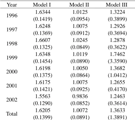
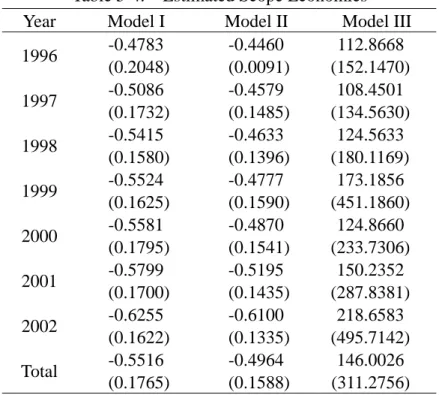
5.4 Economies of Scale and Scope Estimating Results
The coefficient estimates can be used to characterize the dual cost function and the underlying production technology. Overall economies of scale and product mix for each year are calculated and shown in Tables 5-3 and 5-4. A measure of OSE provides useful information to regulators and managers in assessing the potential benefits of mergers and acquisitions. The estimates of OSE from Model I decline slightly during the sample period, while all estimates exceed unity, implying that economies of size prevail in the entire industry. This possible cost advantage resulting from scale economies seems not to be exhausted as the OSE estimates decrease very slowly with the expansion of the industry over time.
[Insert Table 5-3 Here]
The other two models reach quite different results. The estimates of OSE from Models II and III are insignificantly different from unity, i.e., sample banks exhibit constant returns to scale. They are already producing at the minimum point of the long-run average cost curve. No further decrease in average cost is possible, other things being constant. Risk attitudes are inclined to affect the OSE measures.
11
In particular, their TE scores derived from the fixed-effect and the random effect models are about 65.4% and 67.1%, respectively.
Based on equations (2.11) and (2.12), banks cut their optimal outputs in response to risk due to the emergence of terms MRP , 1, i i= 2, leading banks’ output quantities to be under-produced so that their production scale tends to locate on the decreasing portion of the long-run average curve. In contrast, Models II and III do not have the terms MRP shown in their first-order conditions.i 12 Hence, their profit-maximizing outputs are apt to be higher than Model I’s, making their productions’ scales closer to the optimal plant size.
[Insert Table 5-4 Here]
Figures from Models I and II, shown in Table 5-4, draw a different picture from those of Model III. The first two models’ evidence suggests that it is not profitable for banks to produce all types of output jointly, which is consistent with Huang and Wang (2004), who employed the Fourier flexible cost function to examine the panel data on 22 domestic banks in Taiwan with a different data source from the one here. Neither scope economies nor scope diseconomies are found by Model III, which is in compliance with the findings of Huang and Wang (2001) using the same standard fixed-effect model under certainty. It may be viable for risk-averse banks to specialize in the production of either loans or investments. The rejection of joint production is ascribable to the output price uncertainty, which shrinks the optimal level of output and prevents the advantage of cost reductions due to products’ diversification from being effective. This argument seems to be confirmed by Model III in which both products are over-manufactured in terms of the equilibrium outputs under risk, while the total cost of joint production does not deviate significantly from the sum of the total costs incurred by two specialized banks producing the same level of outputs.13
We also calculate the own price elasticities for the three factors of production. All figures are negative, consistent with microeconomic theory. In addition, the computed Allen-Uzawa partial elasticities of substitution unanimously reflect that the pairs of inputs (X1 X ) and (2 X2 X ) are substitutable by the three models.3 14
12
It is important to note that Model II is still affected by the joint probability distribution of random prices P1 and P2.
13
We also compute the measures of cost complementarities, proposed by Baumol et al. (1982). Similar implications to the estimates of scope economies can be drawn and, hence, are overlooked to save space.
14
The commonly-used Allen-Uzawa partial elasticity of substitution between inputs i and j is defined as * * * * * * * ln , , , 1, 2, 3, ln ij j ij i j i i i C C C C S i j C C W C W ∂ = = ≠ = ∂ i j (3.6)
Model I claims that inputs X and 1 X are complements, while Models II and III 3 disagree. These numbers are not shown, but are available upon request to the authors.
6. Concluding Remarks
The current paper proposes a behavioral model of profit maximization under output prices’ uncertainty and safety-first practice. The adopted theoretical model allows for multiple output prices to be stochastic, which is particularly useful in examining financial institutions, such as banks and insurance companies, whose output prices are usually subject to various risks like loan defaults and investment losses. It is therefore necessary to formally consider managers’ risk preferences in order to correctly characterize the influences of risk on a decision-making unit’s equilibrium conditions. In the context of the theoretical model, a system of simultaneous equations is deduced, consisting of a cost and two price equations. The system of equations is in accordance with the assumption of profit maximization and contains extra insightful information on the level of risk and the decision maker’s level of risk aversion. What is more important is that both the levels of risk and risk aversion take an explicit form and, hence, are estimable. Their estimates can be further used to calculate the amount of risk premiums that represents additional costs, which are responsible for the reduction of economic well-being and the fall of outputs.
Given that the subjective probability is significantly estimated and that the risk-averse and safety-first bank behaviors are compatible with the data, Model I -- accounting for the effects of risk -- is more relevant than the other two models. Since the risk premiums are found to be quite substantial and gradually decreasing over time, the creations of a more orderly and responsive financial system and of more transparent banking practices can help lower production costs and promote economic efficiency. However, risk attitudes are found to have little impact on a bank’s TE estimates. In addition, Model III, derived under certainty, tends to overestimate the TE scores.
Evidence is found that overall scale economies prevail in the banking sector of Taiwan, based on the risk-averse Model I. It is advantageous to expand a bank’s production scale through, for example, mergers and acquisitions, indicating that the
where , and . If is greater (less) than zero, then the two
inputs are said to be substitutes (complements). The own price elasticities , must be negative in congruent with standard theory.
* *
i i
C = ∂C ∂W Cij* = ∂2C* ∂ ∂W Wi j Sij
ii
current level of outputs is deficient. At the same time, Models II and III uncover that sample banks are producing at their minimum long-run average cost. Constant returns to scale are pervasive in the sector, while attitudes toward risk play a pivotal role in the determination of an optimal scale of production. A risk-averse decision maker should alternatively pick a larger plant size to take full advantage of scale economies. Based on the estimates of scope economies, it is conservatively inferred that joint production is not preferable. To sum up, the empirical study reveals that a specialized bank providing either loans or investments with a larger scale of production will be better off. This is especially true when banks are undergoing uncertain output prices of all kinds.
This paper extends the theory of a firm to account for responses to multiple output prices’ risk in such a way as to enrich the theoretical framework, to gain further insights on a firm’s behavior, and to broaden our capacity in conducting rigorous empirical research. Researchers should have quantitative evidence through empirical studies to justify the economic implications drawn from a theoretical model and to evaluate the welfare and performance effects of uncertain output prices on cost reductions, optimal output quantities, technical efficiency, and scale and scope economies. Future research could further generalize to examine the cases of multiple input prices’ risk and quality of input risk.
Appendix 1. Derivation of the Second-order Conditions and Comparative Static
Rewrite equations (2.11) and (2.12) as
(
)
1(
)
* 1 2 2 2 * 1 P1 Y1σ11 Y2σ22 2Y Y1 2σ12 Y1σ11 Y2σ12 C1 0 − − Π = + Φ + + + − = , (A1) and(
)
1(
)
* 1 2 2 2 2 P2 Y1σ11 Y2σ22 2Y Y1 2σ12 Y2σ22 Y1σ12 C2 0 − − Π = + Φ + + + − * = . (A2) Taking partial differentiations with respect to Y1 and Y , one obtains 2(
)
2 * 1 3 1 1 * 11 σ Y1σ11 Y2σ12 σ σ11 C11 0 − − − − Π = −Φ + + Φ − ≤ (A3)(
)(
)
* 1 3 1 1 12 σ Y1σ11 Y2σ12 Y2σ22 Y1σ12 σ σ12 C12 − − − − Π = −Φ + + + Φ − * (A4)(
)
2 * 1 3 1 1 * 22 σ Y2σ22 Y1σ12 σ σ22 C22 0 − − − − Π = −Φ + + Φ − ≤ . (A5)Let us perform the comparative static study to find the slopes of the two supply functions and . By totally differentiating equations (A1) and (A2) and through some manipulations, we get
1 Y Y2 * * 11dY1 12dY2 dP1 Π + Π = − , (A7) and * * 12dY1 22dY2 dP2 Π + Π = − , (A8) or in matrix form * * 1 1 11 12 * * 2 2 12 22 dY dP dY dP Π Π − = Π Π − .
It can be shown that
* 1 22 1 0 dY dP −Π = ≥ ∆ , (A9) * 2 12 1 2 dY dY dP dP Π = = ∆ 1 , (A10) and * 2 11 2 0 dY dP −Π = ≥ ∆ . (A11)
The supply functions are upward sloping if the second-order conditions for maximizing profit are satisfied.
It is interesting to note that if dP1=dP2, then 1 2 * 12 * * * 22 1 1 1 1 dP dP dY dP = − Π − Π −Π + Π22 12 = = ∆ ∆ , (A12) and 1 2 * 11 * * * 12 2 1 1 1 dP dP dY dP = Π − Π − −Π + Π11 12 = = ∆ ∆ . (A13)
The signs of (A12) and (A13) are indeterminate and depend on the sign of and its magnitude.
* 12
Appendix 2. Fixed-Effect Estimates
Variable
Name Model I Model II Model III
Variable
Name Model I Model II Model III
U1 10.1429 (7.2385) 8.6820 (7.8494) 33.6250*** (9.8898) U26 12.3447 (7.1745) 10.2999 (7.8579) 36.1386*** (9.9669) U2 10.4194 (7.2507) 9.0875 (7.8626) 33.8980*** (9.9031) U27 10.0193 (7.2601) 9.2289 (7.8758) 33.8089*** (9.9312) U3 11.1450 (7.2145) 8.8633 (7.8209) 34.0105*** (9.7696) U28 10.0395 (7.2564) 9.2194 (7.8737) 33.8011*** (9.9330) U4 10.7288 (7.2233) 9.1172 (7.8267) 34.1567*** (9.8978) U29 10.3297 (7.2584) 9.3398 (7.8664) 34.0679*** (9.9311) U5 10.9419 (7.2224) 8.9971 (7.7980) 33.9107*** (9.8097) U30 10.2544 (7.2503) 9.2806 (7.8652) 33.9828*** (9.9305) U6 11.0553 (7.2309) 9.1732 (7.8225) 33.8978*** (9.8100) U31 10.2395 (7.2480) 9.2361 (7.8694) 34.0140*** (9.9311) U7 11.0166 (7.2353) 9.1714 (7.8227) 34.1792*** (9.8330) U32 10.4588 (7.2429) 9.4153 (7.8663) 34.0783*** (9.9225) U8 10.9876 (7.2540) 9.0689 (7.8237) 34.1368*** (9.8391) U33 10.4651 (7.2452) 9.2215 (7.8602) 34.1277*** (9.9283) U9 10.9901 (7.2462) 9.1594 (7.8328) 34.1665*** (9.8412) U34 10.4215 (7.2481) 9.4279 (7.8643) 34.1302*** (9.9251) U10 10.7136 (7.2275) 9.1088 (7.8154) 34.1166*** (9.8887) U35 10.3677 (7.2577) 9.2942 (7.8682) 34.0383*** (9.9342) U11 10.8821 (7.2188) 9.1428 (7.8408) 34.2518*** (9.8959) U36 10.2279 (7.2457) 9.3233 (7.8653) 34.0100*** (9.9277) U12 10.8317 (7.2523) 9.2735 (7.8461) 34.2899*** (9.9281) U37 10.2458 (7.2592) 9.3463 (7.8584) 34.0048*** (9.9288) U13 10.6282 (7.2502) 9.1509 (7.8484) 34.1149*** (9.9351) U38 9.9600 (7.2525) 9.2604 (7.8739) 33.7879*** (9.9269) U14 10.8071 (7.2627) 9.1923 (7.8429) 34.0124*** (9.8624) U39 10.9538 (7.2529) 9.2164 (7.8389) 34.3325*** (9.8875) U15 10.3861 (7.2589) 9.1729 (7.8632) 33.9731*** (9.9285) U40 10.3980 (7.2470) 9.2397 (7.8488) 34.1345*** (9.9265) U16 10.5274 (7.2516) 9.4329 (0.00001) 34.1295*** (9.9298) U41 10.6500 (7.2596) 9.4659 (7.8617) 34.3860*** (9.9264) U17 10.4046 (7.2473) 9.5763 (7.8680) 33.9182*** (9.9445) U42 10.5065 (7.2415) 9.4086 (7.8568) 34.1139*** (9.9332) U18 10.2492 (7.2456) 9.4770 (7.8646) 34.1090*** (9.9275) U43 10.2892 (7.2415) 9.3985 (7.8651) 34.0409*** (9.9240) U19 10.4523 (7.2138) 9.3651 (7.8532) 34.2390*** (9.9113) U44 10.4008 (7.2704) 9.3547 (7.8652) 33.9112*** (9.9275) U20 10.0999 (7.2468) 9.3631 (7.8785) 33.8064*** (9.8859) U45 10.2160 (7.2313) 9.2901 (7.8547) 33.7569*** (9.9053) U21 9.8758 (7.2506) 9.2889 (7.8588) 33.6799*** (9.8821) U46 9.8597 (7.2674) 9.4759 (7.8936) 33.7482*** (9.9279) U22 10.2476 (7.2492) 9.3023 (7.8750) 34.0389*** (9.9338) U47 10.1035 (7.2584) 9.2759 (7.8760) 33.7675*** (9.9254) U23 10.2963 (7.2507) 9.3001 (7.8658) 34.0657*** (9.9307) U48 10.1806 (7.2623) 9.1940 (7.8758) 33.6506*** (9.9189) U24 9.9038 (7.2550) 9.2034 (7.8780) 33.7040*** (9.9288) U49 10.3244 (7.2783) 9.3230 (7.8560) 33.9615*** (9.9159) U25 10.0513 (7.2538) 9.4485 (7.8750) 33.9191*** (9.9302)
References
Antonovitz, F. and T. Roe (1986), “A theoretical and empirical approach to the value of information in risky markets,” Review of Economics and Economics, 68, 105-114.
Appelbaum, E. (1991), “Uncertainty and the measurement of productivity,” Journal of Productivity Analysis, 2f, 157-17.
Appelbaum, E. and E. Katz (1986), “Measures of risk aversion and the comparative statics of industry equilibrium,” American Economic Review, 76, 524-529.
Appelbaum, E. and U. Kohli (1993), “Import price uncertainty and the distribution of income,” Review of Economics and Statistics, 79, 620-630.
Appelbaum, E. and A. Ullah (1997), “Estimation of moments and production decisions under uncertainty,” Review of Economics and Statistics, 79, 631-637. Ballivian, M.A. and R.C. Sickles (1994), “Product diversification and attitudes toward
risk in agricultural production,” Journal of Productivity Analysis, 5, 271-286. Batra, R.N. and A. Ullah (1974), “Competitive firm and the theory of input demand
under price uncertainty,” Journal of Political Economy, 82, 537-548.
Battese, G.E., A.N. Rambaldi, and G.H. Wan (1997), “A stochastic frontier production function with flexible risk properties,” Journal of Productivity Analysis, 8, 269-280. Baumol, W.J., J.C. Panzar, and R.D. Willig (1982), Contestable markets and the
theory of industry structure, New York: Harcourt Brace Jovanovich.
Berger, A.N. (1993), “Distribution-free estimates of efficiency in the U.S. banking industry and tests of the standard distributional assumptions,” Journal of Productivity Analysis, 4, 261-292.
Chambers, R.G. (1983), “Scale and productivity measurement under risk”, American Economic Review, 73, 802-805.
Dalal, A.J. (1990), “Symmetry restrictions in the analysis of the competitive firm under price uncertainty,” International Economic Review, 31, 207-211.
Hartman, R. (1975), “Competitive Firm and the Theory of Input Demand under Price Uncertainty:Comment,” The Journal of Political Economy, 83, 1289-1290.
Hartman, R. (1976), “Factor Demand with Output Price Uncertainty,” The American Economic Review, 66, 675-681.
Holthausen, D.M. (1976), “Input choices and uncertain demand,” American Economic Review, 66, 94-103.
Huang, C. J. and T.T. Fu (2001), “Uncertainty, risk premium, and productivity in the Taiwan banking industry,” manuscript。
Huang, T.H. and M.H. Wang (2001), “Measuring scale and scope economies in multiproduct banking – A stochastic frontier approach,” Applied Economics Letters,
8, 159-162.
Huang, T.H. and M.H. Wang (2002), “Comparison of economic efficiency estimation methods: Parametric and non-parametric techniques,” The Manchester School, 70, 682-709.
Huang, T.H. and M.H. Wang (2004), “Estimation of scale and scope economies in multiproduct banking: Evidence from the Fourier flexible functional form with panel data,” Applied Economics, 36, 1245-1253.
Hughes, J.P. and L.J. Mester (1998), “Bank capitalization and cost: Evidence of scale economies in risk management and signaling,” Review of Economics and Statistics, 80, 314-325.
Ishii, Y. (1978), ”One the theory of competitive firm under price uncertainty: Note,” American Economic Review, 67, 768-769.
Just, R. (1974), “An investigation of the importance of risk in farmers’ decisions,” American Journal of Agricultural Economics, 56, 14-25.
Just, R.E. and R.D. Pope (1978), “Stochastic specification of production functions and economic implication,” Journal of Econometrics, 7, 67-86.
Kim, H.Y. (1986), “Economies of scale and economies of scope in multiproduct financial institutions: Further evidence from Credit Union,” Journal of Money, Credit, and Banking, 18, 220-226.
Kumbhakar, S. C. (1993), “Production risk, technical efficiency, and panel data,” Economics Letters, 41, 11-16.
Mester, L.J. (1996), “A study of bank efficiency taking into account risk-preferences,” Journal of Banking and Finance, 20, 1025-1045.
Parkin, M. (1970), “Discount house portfolio and debt selection,” Review of Economic Studies, 37, 469-497.
Robison, L.J. and P.J. Barry (1987), The Competitive Firm’s Response to Risk, Macmillan Publishing Company, New York, U.S.A.
Roosen, J. and D.A. Hennessy (2003), “Tests for the role of risk aversion on input use,” American Journal of Agricultural Economics, 85, 30-43.
Roy, A.D. (1952), “Safety first and the holdings of assets,” Econometrica, 20, 431-449.
Sandmo, A. (1971), “On the theory of the competitive firm under price certainty,” American Economic Review,61,65 –73.
Smith, K.R. (1970), “Risk and the optimal utilization of capital,” Review of Economic Studies, 37, 253-259.
Telser, L.G. (1955), “Safety first and hedging,” Review of Economic Studies, 1-16. Turnovsky, S.J. (1973), “Production flexibility, price uncertainty, and the behavior of
Tveteras, R. (1999), “Production risk and productivity growth: Some findings for Norwegian salmon aquaculture,” Journal of Productivity Analysis, 12, 161-179. Viaene, J.M. and I. Zilcha (1998), “The behavior of competitive exporting firms under
multiple uncertainty,” International Economic Review, 39, 591-609.
Wolak, F.A. and C.D. Kolstad (1991), “A model of homogeneous input demand under price uncertainty,” American Economic Review, 81, 514-538.
Table 4-1. Sample Statistics
Variable Name Mean Standard Deviation
*Investments (Y ) 1 48,112,499.98 71,363,582.45 *Loans (Y ) 2 274,722,496.80 306,832,965.40
Price of Y1 ( P ) 1 0.07798 0.09303
Price of Y2 ( P ) 2 0.07668 0.05417
*Net Fixed Assets (X ) 3 7,516,856.39 10,424,739.00 *Deposits and Borrowed
Money (X ) 1 327,090,099.00 363,235,676.70 Full-Time Equivalent Employees (X ) 2 2,232.97 1,890.78 Price of X (W ) 3 3 0.61015 0.63145 Price of X (W ) 1 1 0.04569 0.01460 Price of X (W ) 2 2 966.13 283.25 *Total Costs 19,948,273.56 21,988,191.57 Cost Share of X 3 0.16967 0.09720 Cost Share of X 1 0.70377 0.10252
* Measured in thousands of New Taiwan’s Dollars, deflated by CPI with base year 2001. Number of Observations: 324.
Table 5-1. Parameter Estimates
Model I Model II Model III Variable Name Estimate
(Standard Error) Estimate (Standard Error) Estimate (Standard Error) 11 σ 0.0022** (6.72E-05) 0.0003** (1.35E-04) 22 σ 0.0002** (2.00E-05) 0.00003** (4.27E-05) 33 σ 0.0262** (2.14E-03) 0.0054** (0.0006) 12 σ 0.0001 (6.76E-05) 0.00001 (1.10E-04) 23 σ 0.0011** (1.57E-04) -0.0003** (4.85E-04) 13 σ 0.0005 (1.11E-03) -0.0002 (0.0002) 1 ln y -0.5325** (0.0536) -0.5757** (0.0680) 1.3027*** (0.4693) 2 ln y 0.7343** (0.3618) 0.7892* (0.3542) -4.9092*** (0.8773) 1 ln w 0.4893 (0.4776) 1.2586** (0.4700) -0.0935 (0.4020) 2 ln w 0.7240 (1.1415) 0.6839 (1.0636) -1.2536* (0.6719) 2 1 ln y -0.0450** (0.0032) -0.0104** (0.0044) 0.1631*** (0.0331) 1 ln y ln y 2 0.0451** (0.0028) 0.0125** (0.0057) -0.2852*** (0.0384) 2 2 ln y -0.0725** (0.0137) -0.0400** (0.0107) 0.6249*** (0.0504) 1 ln w ln w 2 -0.0277 (0.0529) -0.0195 (0.0323) 0.0247 (0.0271) 1 ln w ln w 3 0.0899 (0.0566) 0.0680 (0.0477) 0.0409 (0.0366) 2 ln w ln w 3 0.0834 (0.1066) 0.0954 (0.0789) 0.1671*** (0.0650) 1 ln w ln y 1 0.0018 (0.0037) 0.0017 (0.0043) -0.0310** (0.0152) 2 ln w ln y 1 -0.0479** (0.0065) -0.0629** (0.0066) -0.1198*** (0.0395) 1 ln w ln y 2 -0.0540** (0.0131) -0.0911** (0.0114) 0.0320 (0.0207) 2 ln w ln y 2 -0.6190 (0.0335) 0.0039 (0.0286) 0.1110** (0.0509) 0 k 0.0025 (0.0026) 1 k 0.0057** (0.0023) Log likelihood 2530.00 2440.37 268.963
Note: Numbers in parentheses are standard errors.
*: Significant at the 10% level. **: Significant at the 5% level. ***: Significant at the 1% level.
Table 5-2. Estimated Average Risk Premiums Year Index of Risk-aversion
(−Φ−1( *)T )
Risk Premium
(Millions of 2001 NT dollars)
Rate of Risk Premium (%) 1996 2.81 12244.7 47.72 1997 2.40 10426.3 46.84 1998 2.20 10287.0 41.94 1999 2.06 9844.0 41.05 2000 1.95 9245.5 40.24 2001 1.86 9305.1 40.58 2002 1.79 9111.4 46.14 Total 2.15 10001.8 43.35
Table 5-3. Estimated Scale Economies
Year Model I Model II Model III
1996 1.6344 (0.1419) 1.0125 (0.0954) 1.3224 (0.3899) 1997 1.6248 (0.1369) 1.0075 (0.0912) 1.2926 (0.3694) 1998 1.6607 (0.1325) 1.0245 (0.0849) 1.2878 (0.3622) 1999 1.6348 (0.1454) 1.0119 (0.0890) 1.7462 (3.3590) 2000 1.6198 (0.1375) 1.0050 (0.0864) 1.3682 (1.0412) 2001 1.6175 (0.1421) 1.0075 (0.0925) 1.2655 (0.4170) 2002 1.5563 (0.1290) 0.9836 (0.0852) 1.2463 (0.3614) Total 1.6205 (0.1399) 1.0072 (0.0891) 1.3633 (1.3891) Standard deviations are shown in the parentheses.
Table 5-4. Estimated Scope Economies
Year Model I Model II Model III
1996 -0.4783 (0.2048) -0.4460 (0.0091) 112.8668 (152.1470) 1997 -0.5086 (0.1732) -0.4579 (0.1485) 108.4501 (134.5630) 1998 -0.5415 (0.1580) -0.4633 (0.1396) 124.5633 (180.1169) 1999 -0.5524 (0.1625) -0.4777 (0.1590) 173.1856 (451.1860) 2000 -0.5581 (0.1795) -0.4870 (0.1541) 124.8660 (233.7306) 2001 -0.5799 (0.1700) -0.5195 (0.1435) 150.2352 (287.8381) 2002 -0.6255 (0.1622) -0.6100 (0.1335) 218.6583 (495.7142) Total -0.5516 (0.1765) -0.4964 (0.1588) 146.0026 (311.2756) Standard deviations are shown in the parentheses.