頻寬-空間-極化於寬頻多輸入多輸出無線電通道影響之研究

(1)

國立交通大學

電信工程學系

博士論文

頻寬-空間-極化於寬頻多輸入多輸出無線電

通道影響之研究

Effects of Bandwidth-Space-Polarization on

UWB/Wideband Multiple-Input Multiple-Output

Channels

研究生：張維儒

指導教授：唐震寰博士

(2)

頻寬-空間-極化於寬頻多輸入多輸出無線電

通道影響之研究

Effects of Bandwidth-Space-Polarization on

UWB/Wideband Multiple-Input

Multiple-Output Channels

研究生：張維儒

Student:

Wei-Ju

Chang

指導教授：唐震寰博士 Advisor:

Dr.

Jenn-Hwan

Tarng

國立交通大學

電信工程學系

博士論文

A Dissertation

Submitted to Institute of Communication Engineering

College of Electrical and Computer Engineering

National Chiao Tung University

in Partial Fulfillment of the Requirements

for the Degree of Doctor of Philosophy

in

Communication Engineering

Hsinchu, Taiwan

(3)

頻寬-空間-極化於寬頻多輸入多輸出無線電

通道影響之研究

研究生：張維儒指導教授：唐震寰博士

國立交通大學電信工程學系

中文摘要

為滿足下一代(B3G)無線通信系統的高傳輸速率需求，使用高頻寬並搭配多輸入多輸出(MIMO)天線技術是未來無線通信系統的發展趨勢，而其通道特性的掌握與適當模型的建構更是B3G 無線通信系統發展之初的首要課題。對寬頻MIMO 通道而言，頻寬、天線間距及天線極化是影響其通道模型參數的主要因子。頻寬的增加代表系統時間解析度變好，多路徑延遲(multipath delay)及群聚 (clustering)現象越明顯，窄頻之多路徑延遲模型必須修正以滿足寬頻系統通道之需求；而在多天線部份，除空間天線陣列架構外，極化天線的應用有助於在無線終端設備上實現多天線架構，因此，完整考量Space-Polarization 相關性的 MIMO 通道模型，是MIMO 技術設計發展所必需。

(4)

本論文完整探討Bandwidth-Space-Polarization 對寬頻 MIMO 通道之影響，發展一創新之寬頻通道模型參數預估方法，可由窄頻通道模型參數預估寬頻通道參數模型。另外吾人也針對室內環境，發展三維空間幾何散射模型，該模型結合幾何圓模型與幾何橢圓模型之概念並將之拓展至三維空間，可用以模擬空間/極化陣列天線 MIMO 通道的相關性。除此，吾人也透過實測數據分析，探討 UWB-MIMO 於身域環境(BAN) 之效能。本研究所發展之寬頻通道模型參數預估方法與MIMO 通道相關性模型，皆經由實測數據分析獲得驗證，實測環境包含室外寬頻(120 MHz)、室內及身域環境之超寬頻(3-10 GHz 頻段)通道量測，完全符合下一代無線通信系統之需求。

(5)

Effects of Bandwidth-Space-Polarization on

UWB/Wideband Multiple-Input

Multiple-Output Channels

Student:

Wei-Ju

Chang Advisor:

Dr.

Jenn-Hwan

Tarng

Institute of Communication Engineering

National Chiao Tung University

Abstract

To achieve high data rate requirements of systems beyond 3rd generation (B3G),

development and standardization of enhanced radio access technologies with wide

bandwidth and multiple-input multiple-output (MIMO) antennas are sustained. In wireless

communication systems, radio channels play an important role on system performance.

Therefore, a through understanding of wideband MIMO channel characteristics is essential

for B3G wireless systems developing and realization.

Compared to traditional narrowband single-input single-output (SISO) channels,

bandwidth, array spacing and antenna polarization effects should be taking into account in

(6)

to observe more multipath components, and therefore stronger clustering effects due to its

better time resolution. For MIMO systems, in addition to spatial arrays, the utilization of

polar arrays is of great interest recently due to its benefit to the device compactness.

Therefore, a complete MIMO channel model should include the space factor as well as the

polarization factors.

In this research, effects of bandwidth-space-polarization on UWB/wideband MIMO

channels are investigated. Here, a novel method for wideband model parameters estimation

is developed. Through this method, the model parameters of a wideband signal can be

determined from those of a narrowband signal. Furthermore, a three-dimensional

Geometrically Based Single Bounce Model (3D GBSBM), is proposed for indoor wideband

MIMO channel correlation modeling. This model is extended from a 2D model, which

combines the concept of the Geometrically Based Single Bounce Circle Model (GBSBCM)

and the Geometrically Based Single Bounce Ellipse Model (GBSBEM). In this model, the

effect of 3D multipath on sub-channel correlation of the spatial/polar arrays is taken into

account. Finally, the performance of UWB-MIMO for body area networks (BANs) is

investigated through channel measurements.

The newly developed method and models are validated by broadband channel

(120-MHz bandwidth) measurements in outdoors as well as ultra-wideband channels (3-10

(7)

誌

謝

本論文得以順利完成，有賴生命中許許多多貴人的指導、協助、包容與相伴，於此，以感恩之心，謹將此論文獻給您們！首先，我要以最誠摯的敬意感謝我的指導老師唐震寰教授，承蒙老師自大學、碩士至博士多年來的指導，讓我在無線電傳播的專業知識領域多有成長，並能在相關研究上有所突破，老師嚴謹認真的治學精神與謙沖的待人處事態度更是學生的典範。其次，本論文相關研究工作得以順利進行，也有賴實驗室瑞榮學長的指導，以及學弟妹豐誠、鳴君、孟勳、思云等人的共同努力，感謝他們。當然，也要特別感謝梁小姐麗君多年來在各項事務上的熱心協助。另外，也要感謝本論文的口試委員李大嵩教授、李學智教授、張道治教授、彭松村教授、楊成發教授，能在百忙當中撥冗費心審查，對論文內容提出懇切的意見與指導，讓本論文能更臻完善。於此，也要特別感謝陳榮義主任的提攜與推薦，讓我有機會完成博士學位的進修。計畫主管與同事在工作上給予的包容與協助，我更是銘感於心，每位同事的專業素養，也讓我在通訊知識上能不斷成長。最後，我要將此喜悅與我最親愛的家人分享。母親自小全心全意的照顧與教誨，讓我能以樂觀進取之心平順克服學業與職場的挑戰，而我親愛的老婆欣怡與女兒詠瑜，更是我精神上最大的支柱，有妳們陪伴的每一天，生活中總是歡樂喜悅與滿滿的幸福，我愛妳們也謝謝妳們。

(8)

List of Tables

Chapter 2 Overview of Channel Models for B3G Systems………..7

Table 2-1 The channel parameters of 3GPP SCM for link level simulations…… 28

Table 2-2 The channel parameters of 3GPP SCM for system level simulations…29 Table 2-3 Sub-paths to mid-paths assignment and resulting angle spread in 3GPP SCME……….……. 30

Chapter 3 Measurement and Modeling of Wideband SISO Channels………. 32

Table 3-1 Setup and environments for the broadband outdoor channel measurements……….………... 46

Table 3-2 Values of me-λ, σe-λ, me-P and σe-P for n=2……….. 61

Table 3-3 Values of me-λ, σe-λ, me-P and σe-P for n=4……….. 61

(11)

List of Figures

Chapter 1 Introduction………...1

Fig. 1-1 A diagram of 3GPP standard evolution….………...….4

Chapter 2 Overview of Channel Models for B3G Systems………..7

Fig. 2-1 The illustration of the ∆-K process……….………... 13

Fig. 2-2 The illustration of exponential decay of mean cluster power and ray power within clusters………. 15

Fig. 2-3 The illustration of the geometry of Lee’s model………. 17

Fig. 2-4 The illustration of the geometry of GBSBCM……… 18

Fig. 2-5 The illustration of the geometry of GBSBEM………. 20

Fig. 2-6 The illustration of the procedure for generating MIMO channels………... 30

Fig. 2-7 The illustration of multipath angle parameters at BS and MS sides…….... 31

Fig. 2-8 A diagram of the mid-path approach of SCME………... 31

Chapter 3 Measurement and Modeling of Wideband SISO Channels………. 32

Fig. 3-1 A diagram for bandwidth effect on the observed multipath propagation channels………34

Fig. 3-2 A diagram for the arrival of multipath when bandwidth changes from F to f for n=2……….…..38

Fig. 3-3 The averaged power delay profile of a 500 MHz-bandwidth UWB signal at an indoor environment and under NLOS condition. The wavy line shows the measured profile. The straight line, which is obtained by a best-fit procedure, represents an exponential decay line………. 40

Fig. 3-4 Rician factors of the first 15 bins of each measured point at indoor environments with 2-GHz bandwidth are shown. The total numbers of measured points are 24……… 41

(12)

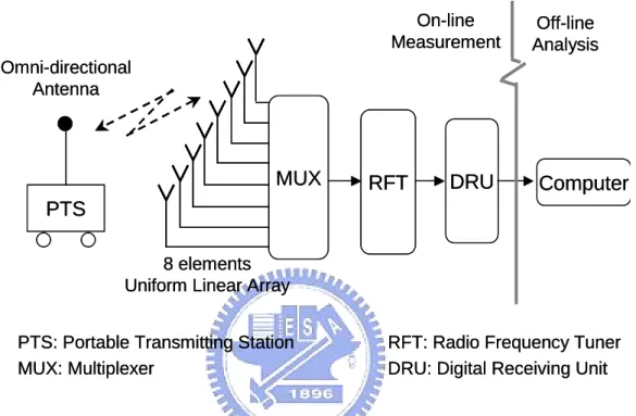
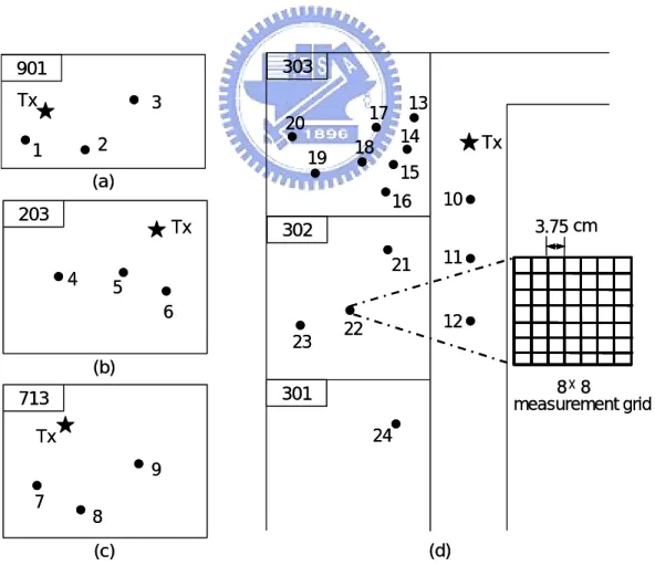
Fig. 3-6 Schematic diagram of the UWB indoor channel measurement system….. 49 Fig. 3-7 Layouts of four sites where the UWB indoor channel measurements were

performed. Locations of the transmitter (Tx) and the receiver are shown by “Ì” and “•”, respectively………... 49 Fig. 3-8 Comparisons of the measured and computed results of (a) the path arrival

rate λi; and (b) the path occurrence probability Pi of “Urban 1” site with 60-MHz bandwidth for n=2……… 58 Fig. 3-9 Comparisons of the measured and computed results of (a) the path arrival

rate λi; (b) the path occurrence probability Pi of “Indoor NLOS” site with 1 GHz bandwidth for n=2……… 59 Fig. 3-10 Comparisons of the measured and computed results of (a) the path arrival

rate λi; (b) the path occurrence probability Pi of “Urban 1” site with 120 MHz bandwidth for n=4……….. 60 Fig. 3-11 The measured ki of “Indoor NLOS” site with 1 GHz bandwidth………...62 Fig. 3-12 K value of the measurement sites: (a) outdoor environments; and (b)

indoor environments……… 63 Fig. 3-13 Decay constant versus measured point number for signal bandwidths of

500MHz, 1GHz, and 2GHz at “Indoor LOS” and “Indoor NLOS” sites… 65 Fig. 3-14 Power ratio versus measured point number for signal bandwidths of 500

MHz, 1GHz, and 2GHz at “Indoor LOS” and “Indoor NLOS” sites…….. 66 Fig. 3-15 Comparisons between the measured and computed results of the power

ratio for all measured points at “Indoor LOS” and “Indoor NLOS” sites with 1GHz bandwidth……….. 66 Fig. 3-16 Rician factor versus measured point number for signal bandwidths of

500MHz, 1GHz, and 2GHz at “Indoor LOS” and “Indoor NLOS” sites… 67 Fig. 3-17 Comparisons between the measured and computed results of the Rician

factor for all measured points at “Indoor LOS” and “Indoor NLOS” sites with 1GHz bandwidth……….. 67

Chapter 4 Measurement and Modeling of Space Correlation for Indoor

(13)

Fig. 4-1 Per tap MIMO correlation metrics……….. 73 Fig. 4-2 The illustration of the geometry of the 3D GBSBEM………. 76 Fig. 4-3 Thr geometry for the scatter region of different taps………... 77 Fig. 4-4 The illustration of the geometry of the 3D GBSBM for the 1st tap: (a) the

effective scatter region; (b) the effective scatterers………. 77 Fig. 4-5 The illustration of the geometry of the 3D GBSBM for the 2nd tap: (a) the

effective scatter region; (b) the effective scatterers………. 78 Fig. 4-6 The geometrical configuration of a 1-by-2 channel of the 3D GBSBM…. 84 Fig. 4-7 The illustration of the 3D GBSBM in cylindrical coordinates……… 85 Fig. 4-8 The illustration of the 3D GBSBM for the nth tap………... 85 Fig. 4-9 The simulated spatial correlation of the co-polarized antenna case based

on the 2D GBSBM………... 86 Fig. 4-10 The simulated spatial correlation of the co-polarized antenna case based

on the 3D GBSBM for the 1st tap………. 86 Fig. 4-11 The simulated spatial correlation of the cross-polarized antenna case based

on the 3D GBSBM for the 1st tap………. 87 Fig. 4-12 The simulated spatial correlation of the cross-polarized antenna case based

on the 3D GBSBM for the 5th tap……… 87

Fig. 4-13 Layouts of the wideband MIMO channel measurement site………... 89 Fig. 4-14 The virtual antenna array configuration for MIMO channel

measurements………..……… 90 Fig. 4-15 The measured and fitted CDFs of the normalized power of the 1st tap…... 92 Fig. 4-16 The measured and fitted CDFs of the normalized power of the 2nd tap….. 92 Fig. 4-17 The measured and simulated space correlation of the 1st tap for

co-polarized antenna case……… 93 Fig. 4-18 The measured and simulated space correlation of the 2nd tap for

co-polarized antenna case……… 93 Fig. 4-19 The measured and simulated space correlation of the 1st tap for

cross-polarized antenna case……… 94 Fig. 4-20 The measured and simulated space correlation of the 2nd tap for

(14)

Chapter 5 Measurements and Analysis of UWB MIMO Performance for Body Area Network Applications………... 96

Fig. 5-1 Measured antenna return loss versus frequency………101 Fig. 5-2 The locations of Tx and Rx antennas for MIMO measurements………...101 Fig. 5-3 Floor layouts of measurement sites. (a) Sites A and B; (b) Site C……….102 Fig. 5-4 The measured 2×2 MIMO channel capacity at different sites for frequency

band of 3-10 GHz………...105 Fig. 5-5 The measured 2×2 MIMO channel capacity at site C………106 Fig. 5-6 One sub-channel frequency response at Site C………..106 Fig. 5-7 MIMO channel capacities versus receiving array spacing at Site A……..108 Fig. 5-8 Spatial correlation coefficients versus receiving array spacing at Site A..109 Fig. 5-9 Maximum value of the power differences between any two sub-channels

versus receiving and transmitting array spacing at Site A……….109 Fig. 5-10 The measured 2×2 MIMO channel capacity of the polar array and the

spatial array at Site C……….111 Fig. 5-11 Received power of V/V or V/H link versus frequency at Site C for (a)

(15)

Abbreviations

Abbreviation Description

3G third generation

3GPP 3rd generation partnership project 3GPP2 3rd generation partnership project 2

AoA angle of arrival

AoD angle of departure

aPDP averaged power delay profile

AS angle spread

B3G beyond third generation

BAN body area network

BS base station

DS delay spread

GBSBM geometrically based single bounce model

GBSBCM geometrically based single bounce circular model GBSBEM geometrically based single bounce ellipse model HSDPA high speed downlink packet access

IFFT inverse fast Fourier transform

i.i.d. independently and identically distributed iPDP instantaneous power delay profile

ISI inter-symbol interference

LOS line-of-sight

LTE long-term evolution

METRA multi-element transmit receive antennas

MIMO multiple-input multiple-output

MPC multipath component

MS mobile station

NLOS non line-of-sight

(16)

PDF probability density function

PDP power delay profile

S-V Saleh-Valenzuela

SCM spatial channel model

SCME spatial channel model extension

SF shadow fading

SISO single-input single-output

SNR signal-to-noise ratio

TDL tapped-delay-line

TOA time of arrival

ULA uniform linear array

UWB ultra-wideband

VAN vector network analyzer

WAN wide area network

WLAN wireless local area network

(17)

Chapter 1 Introduction

In this chapter, the motivation and contributions of this research and the overview of this thesis are presented.

(18)

1.1 Motivation and Contributions

Recently, systems beyond 3G (B3G) have been actively discussed in various forum

and organizations. According to the ITU-R preliminary recommendation [1], new radio

interfaces of B3G systems will support high data rate transmissions up to approximately

100 Mbps for high mobility and 1 Gbps for low mobility, respectively. To achieve the high

data rate requirements, standardization and development of enhanced radio access

technologies with wide bandwidth and multiple antennas are sustained.

For instance, 3GPP is in the process of defining the long-term evolution (LTE) [2] and

LTE-Advanced for B3G services. Fig. 1-1 shows the evolution path of 3GPP standards.

Compared to the high-speed downlink packet access (HSDPA) [3] that introduced in 3GPP

release 5, LTE improves the downlink peak data rate from 14.4 Mbps to approximately 300

Mbps by using 4×4 multiple-input multiple-output (MIMO) antenna technologies along

with a wide bandwidth of 20 MHz, which is four times the bandwidth of HSDPA. In

addition to that, to meet the 1-Gbps peak data rate requirements of B3G systems, 3GPP

begins to process the feasibility studies of technologies using 8×8 MIMO along with a

bandwidth of 40 MHz. Furthermore, for short-range communications, ultra-wideband

(UWB) radio technology has attracted great interest in commercial and military sectors due

(19)

transmission bandwidth of 500 MHz at least [4].

The performance of wireless communications is greatly influenced by the radio

propagation channels. Consequently, a thorough understanding of UWB/wideband MIMO

channel characterizations is essential for the realization of B3G systems. To model

UWB/wideband MIMO channels, the statistical properties in frequency (bandwidth) and

spatial domains have to be carefully investigated. Furthermore, cross-polarized antennas

are of interest for MIMO applications due to its potential benefit for the device

compactness. Therefore, a complete investigation of UWB/wideband MIMO channels

should cover the characterizations and effects of bandwidth, space and polarization, which

is also the goal of this research.

For bandwidth effect, our major contribution is to develop a novel method to estimate

the model parameters of a wideband signal from those of a narrowband signal. Through

this approach, the proper model parameters for B3G systems can be determined from those

of current models of 3G systems, which support system bandwidth up to 5 MHz.

Furthermore, for space and polarization effect on MIMO channels, a three-dimensional

Geometrically Based Single Bounce Model (3D GBSBM) is proposed for the space

correlation modeling of indoor wideband MIMO channels. This model is extended from a

2D model, which combines the concept of the Geometrically Based Single Bounce Circle

(20)

In this model, the effect of 3D multipath on sub-channel correlation of the spatial/polar

arrays is taken into account.

Finally, UWB-MIMO performance in body area networks (BAN) is investigated

through channel measurements. It is found that in BAN the MIMO channel capacity is

mainly determined by the power imbalance between sub-channels compared to the

sub-channel correlation for spatial arrays, which is different from that in wide-area

networks (WAN) and wireless local area networks (WLAN).

In this research, the newly developed method and models are validated by extensive

broadband channel (120-MHz bandwidth) measurements in outdoors as well as UWB

channels (3-10 GHz) in indoors and BANs, which is agreeable to the requirements of B3G

systems. HSPA HSPA HSPA+ HSPA+ LTE LTE LTE-Advanced LTE-Advanced 5 MHz 20 MHz 40+ MHz 1×2 SIMO 2×2 MIMO 4×4 MIMO 8×8 MIMO Bandwidth 14.4 Mbps 28 Mbps ~300 Mbps ~1 Gbps HSPA HSPA HSPA+ HSPA+ LTE LTE LTE-Advanced LTE-Advanced 5 MHz 20 MHz 40+ MHz 1×2 SIMO 2×2 MIMO 4×4 MIMO 8×8 MIMO Bandwidth 14.4 Mbps 28 Mbps ~300 Mbps ~1 Gbps

(21)

1.2 Thesis Overview

In Chapter 2, some of the well-known models for wideband multipath delay

propagations and for MIMO channels are introduced. For UWB/wideband propagations,

multipath arrivals in cluster rather than in continuum as is customary for narrowband

channels. The ∆-K model [5] and the Saleh-Valenzuela (S-V) model [6] are two

well-recognized models to characterize the multipath-clustering phenomenon in delay

domain. For MIMO channels, correlation between sub-channels, which is dependent on the

multipath power-angle spectrum and array architecture, is significant to MIMO channel

capacity. The spatial channel models proposed in IEEE 802.11n [7] and 3GPP/3GPP2 [8]

are two representative models for MIMO channels in indoor and cellular environments,

respectively.

In Chapter 3, measurement and modeling of UWB/wideband multipath channels for

single-input single-output (SISO) is described. Here, a novel method is proposed to

estimate the model parameters of a wideband signal from those of a narrowband signal.

Through this approach, effect of bandwidth on the observable multipath-clustering is

explored. Our proposed method is extensively validated by measured channels of 1.95

GHz and 2.44 GHz broadband radios in metropolitan and suburban areas, and of 3-5 GHz

(22)

In Chapter 4, a newly developed 3D GBSBM for indoor environments is introduced.

Based on this model, we derived the correlation between MIMO sub-channels of

spatial/polar arrays and discuss its sensitively to a variety of different azimuth and

elevation angle spreads. By combining this 3D GBSBM scattering model with the

deterministic rays, site-specific indoor MIMO channels are well modeled.

In Chapter 5, the performance of UWB-MIMO applications in BANs in presented.

Here, the effects of bandwidth, array spacing, and antenna polarization on UWB-MIMO

channel capacity are experimentally investigated and discussed.

(23)

Chapter 2 Overview of Channel

Models for B3G Systems

In this chapter, first the well-known models for multipath-clustering are introduced. Then some MIMO channel models presented in literature and standards are introduced.

(24)

2.1 Introduction

Because of multipath propagation due to reflections, refractions, and/or scattering by

obstacles or scatters in propagation environments, radio propagation channels are usually

modeled as a linear filter with a complex-valued lowpass equivalent impulse response that

is expressed as

( )

=∑

(

−

)

k k k

a

hτ δ τ τ (2-1)

where ak and τk are the random complex-valued path gain and propagation delay of the

multipath components (MPCs), respectively; and δ is the Dirac delta function. However, in

practice, bandwidth of a signal is finite consequently the multipath resolution duration is

nonzero and is equal to the reciprocal of the signal bandwidth. Therefore, the number of

resolved multipath and its path gain is dependent on signal bandwidth.

In addition to the time dispersion phenomenon, angular dispersion effects are

described by the double-directional channel impulse response [9]

(

)

(

) (

_l

) (

_l

)

l l l

a

hτ, ,φ ψ =∑ δ τ−τ δ φ−φ δψ −ψ (2-2)

(25)

departure (AoD) and the angle of arrival (AoA), respectively. It is noted that the

double-directional channel impulse response describes only the propagation channel and is

thus independent of antenna.

For MIMO systems, the channel response has to be described for all transmit and

receive antenna pairs. Let us consider MIMO system with m transmit antennas and n

receive antennas, then the time-invariant MIMO channel is represented by a n×m channel

matrix:

( )

⎟⎟ ⎟ ⎟ ⎟ ⎟ ⎠ ⎞ ⎜ ⎜ ⎜ ⎜ ⎜ ⎜ ⎝ ⎛ = τ τ τ τ τ τ τ τ τ τ nm n n m m h h h h h h h h h 2 1 1 22 21 1 12 11 K M O M M K K H (2-3)

where, hij(τ) denote the impulse response between the jth transmit antenna and the ith

receive antenna. It is noted that hij(τ) includes the effects of propagation channel and

antennas. The relationship between hij(τ) in (2-3) and h(τ, φ, ψ) in (2-2) is shown as

( )

τ

(

( ) ( )

τ φ ψ

)

( )

φ

( )

ψ ϕ ψ φ ψ d d G G h h_ij = ∫ ∫ r_Txj ,r_Rxi , , , _Tx _Rx (2-4)

where, r(j)_Tx and r(j)_Rx are the coordinates of the jth transmit and ith receive antenna,

(26)

pattern, respectively.

For cross-polarized antenna applications, the polarization can be take into account by

extending the impulse response to a polarimetric (2×2) matrix [10] that describes the

coupling between vertical (V) and horizontal (H) polarizations:

(

)

(

)

(

)

(

)

(

)

(

) (

l

) (

l

)

l HV _lHH l l VH l VV l HH HV VH VV a a a a h h h h ψ ψ δ φ φ δ τ τ δ ψ φ τ ψ φ τ ψ φ τ ψ φ τ ψ φ τ − − − ⎟⎟ ⎟ ⎠ ⎞ ⎜⎜ ⎜ ⎝ ⎛ = ⎟ ⎟ ⎠ ⎞ ⎜ ⎜ ⎝ ⎛ = ∑ pol , , , , , , , , , , H (2-5)

From (2-4) and (2-5), it is found that the bandwidth, array spacing and antenna

polarization effects should be taking into account in the modeling of wideband MIMO

channels.

2.2 Multipath models for wideband channels

For narrowband/wideband radio channels, the tapped-delay-line (TDL) model is a

well-recognized model for multipath delay propagations. In this model, the axis of excess

delay times is partitioned into bins and the bin width is equal to the reciprocal of the signal

bandwidth. It assumes multipath arrive at every bins with average power profile that

(27)

Multipath-clustering, the phenomenon that multipath arrivals in cluster, has been

found in outdoor broadband channels as well as in indoor UWB channels [5-6, 11-16]. It is

caused by the fact that scatterers tend to group together in realistic environments and are

resolved in groups by the system with fine or very fine time resolution. Modeling of this

phenomenon helps the design of an equalizer or Rake receiver, such as design of equalizers

with unequal tap spacing or design of a selective Rake receiver and partial Rake receivers

[12]. In addition, in [17], it shows that unclustered models tend to overestimate the channel

capacity as comparing with the case that multipath components are indeed clustered. Here,

tow well-recognized models to characterize the multipath-clustering phenomenon, the ∆-K

model and the S-V model, are introduced.

2.2.1 ∆-K model

The ∆-K model is initiated by Turin et al. [18], [19] and developed by Suzuki [5] to

describe the ToAs of MPCs by taking multipath-clustering into account. In the model, the

axis of excess delay times (relative to the propagation delay of the direct path between

transmitting and receiving antennas) is partitioned into bins with width ∆ [5]. The

probability of having a path in bin i is a function of whether or not an arrival occurred in

the previous bin, and is a function of the empirical probability of path occurrences at

(28)

of Fig. 2-1: the probability of having a path in bin i is equal to λi if there is no path in the

(i-1)st bin; otherwise, it is increased by a factor K due to multipath-clustering effect. Note

that, both the path occurrence probabilities, λi and K⋅λi, are equal to or less than 1. When K

>1, the process exhibits a clustering property and large K represents a large clustering

effect. For K=1, this process reverts to a standard Poisson process.

It is noted that this model is applicable upon replacing K by ki, which is a function of

the bin number i [5, 20-21]. From the branching process shown in Fig. 2-1 with replacing

K by ki, it is found that, Pi, the probability of having a path in bin i, is equal to the sum of

the probabilities (1-Pi-1)⋅λi and Pi-1⋅ki⋅λi. After some derivations, λi is given as

2 , 1 1 ⋅ ₁+ ≥ − = − i P k P i i i i ) ( λ (2-6) where λ1 = P1.

It is noted that ∆ is a model parameter to be chosen [5,18]. However, according to the

assumption in these papers that each bin contains either one path or no path, it is

reasonable to set ∆ as the signal time resolution, which is reciprocal of the signal

bandwidth, of the specific radio system [11, 21-22]. This is because two or more paths

arriving within the same time resolution interval cannot be resolved as distinct paths for a

(29)

bandwidths may observe different multipath-clustering phenomenon and yield different

channel model parameters for a specific environment because that the number of

resolvable MPCs and clusters are changed with signal time resolution.

1 λ

…

..

.

∆

bin 1 bin 2 bin 3 bin 4

1 1−λ 2 λ K 2 1−Kλ 2 λ 2 1−λ 3 λ K 3 1−Kλ 3 λ 3 1−λ 3 λ K 3 1−Kλ 3 λ 3 1−λ 4 λ K 4 1−Kλ 4 λ 4 1−λ 1 λ

…

..

.

∆

bin 1 bin 2 bin 3 bin 4

1 1−λ 2 λ K 2 1−Kλ 2 λ 2 1−λ 3 λ K 3 1−Kλ 3 λ 3 1−λ 3 λ K 3 1−Kλ 3 λ 3 1−λ 4 λ K 4 1−Kλ 4 λ 4 1−λ

Fig. 2-1 The illustration of the ∆-K process.

2.2.2 Saleh-Valenzuela model

The S-V model was introduced first by Saleh-Valenzuela [6] to characterize the

multipath-clustering phenomenon, and later verified, extended, and elaborated upon by

many other researchers in [14-15]. The major difference between S-V model and

(30)

time interval. Instead, two Poisson models are employed in the modeling of the arrival time.

The first Poisson model is for the first path of each path cluster and the second Poisson

model is for the paths (or rays) within each cluster. Following the terminology in [6], we

define

Tl = the arrival time of the first path of the l-th cluster;

τk,l = the delay of the k-th path within the l-th cluster relative to the first path arrival

time, Tl;

Λ = cluster arrival rate;

λ = ray arrival rate, i.e., the arrival rate of path within each cluster.

By definition, we have τ₀_l =T_l. The distribution of cluster arrival time and the ray

arrival time are given by (2-2) and (2-3), respectively

(

T T₋₁

)

=Λ

[

−Λ

(

T −T ₋₁

)

]

l >0

p _l _l exp _l _l , (2-7)

(

₋₁

)

=

[

−

(

− ₋₁

)

]

k >0

pτ_k_,_lτ₍_k _),_l λexp λτ_k_,_l τ₍_k _),_l , (2-8)

The magnitude of the k-th path within the l-th cluster is denoted by βkl. It is Rayleigh

distributed with a mean given by

( ) (

)

(

τ γ

)

β

(31)

where Γ and γ are the cluster and ray decay constants, respectively. β2

( )

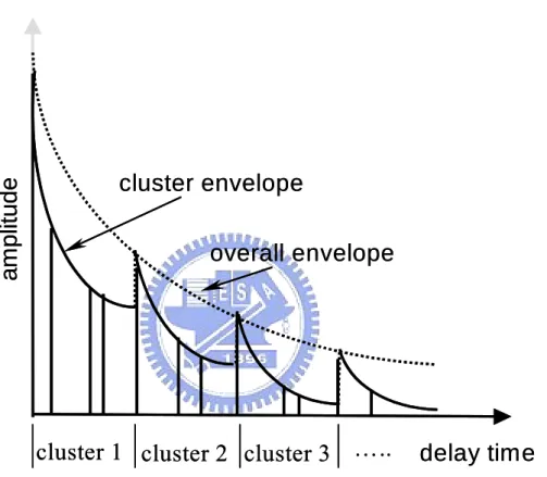
0,0 is the average power of the first arrival of the first cluster. Illustrations of the double exponential

decay model in Fig. 2-2.

delay time

a

m

plitude

overall envelope

cluster envelope

cluster 1 cluster 2 cluster 3 ….. delay time

a

m

plitude

overall envelope

cluster envelope

cluster 1 cluster 2 cluster 3 …..

Fig. 2-2 The illustration of exponential decay of mean cluster power and ray power within clusters.

(32)

2.3 Spatial channel models

2.3.1 Overview of Developed Spatial Channel Models

A. Ray tracing models

In the past few years, a deterministic model, called ray tracing, has been proposed

based on the geometric theory and reflection and diffraction models. By using site-specific

information, this technique deterministically models the propagation channel, including the

path loss, the multipath delay and angle spread. However, the high computational burden

and lack of detailed terrain and building databases make ray tracing models difficult to use.

For computation efficiency, some physical-based models, such as Lee’s model and

geometrically based single bounce models, and analytical-based models, such as

correlation-based model, are developed.

B. Lee’s model

In Lee’s model, scatterers are evenly spaced on a circular ring about the mobile as

shown in Fig. 2-3 [23, 24]. Each of the scatterers is intended to represent the effect of

many scatterers within the region, and hence are referred to as effective scatterers.

Assuming that N scatterers are uniformly placed on the circle with radius R and

(33)

1 1 0 2 ₌ ₋ ⎟ ⎠ ⎞ ⎜ ⎝ ⎛ ≈ i i N N D R i sin , , ,K, π φ (2-10)

From the discrete AoAs, the correlation of the signals between any two elements of

the array can be found using

(

)

∑−

[

(

)

]

= − + = 1 0 0 0 1 2 N i i d j N D R d θ π θ θ ρ , , , exp cos (2-11)

where d is the element spacing and θ0 is measured with respect to the line between the two

elements as shown in Fig. 2-3.

(34)

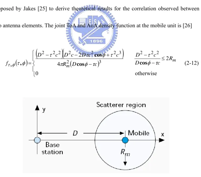
C. Geometrically Based Single Bounce Circular Model

The Geometrically Based Single Bounce Circular Model (GBSBCM) is applicable to

macro-cell scenarios. The geometry of the GBSBCM is shown in Fig. 2-4. It assumes that

the scatterers lie within radius Rm about the mobile. Often the requirement that Rm < D is

imposed. Furthermore, it assumes that there is no scatterer near the base station since the

height of base station antenna is very large relative to scatterers in macro-cell environments.

The idea of a circular region of scatterers centered about the mobile was originally

proposed by Jakes [25] to derive theoretical results for the correlation observed between

two antenna elements. The joint ToA and AoA density function at the mobile unit is [26]

( )

(

)(

₍

₎

)

⎪ ⎩ ⎪ ⎨ ⎧ ≤ − − − + − − = otherwise 0 2 4 2 2 2 2 3 2 3 2 2 2 2 2 2 m m R c D c D c D R c c D c D c D f φ τ τ τ φ π τ φ τ τ φ τ φ τ _cos cos cos , , (2-12)

(35)

D. Geometrically Based Single Bounce Elliptical Model

For micro-cell environments where the base station antenna is at the same height as

the surrounding scatterers, the Geometrically Based Single Bounce Elliptical Model

(GBSBEM) is developed to take into account the effect of scatterers around the base

station antennas [27-28]. In the GBSBEM, it assumes that scatterers are uniformly

distributed within an ellipse, as shown in Fig. 2-5, where the base station and mobile are

the foci of the ellipse. The parameters am and bm are the semi-major axis and semi-minor

axis values, which are implicitly to delay of the maximum ToA to be considered, τm , by

2 2 2 2 b c D c a_m = τ_m , _m = τ_m− (2-13)

where c is the speed of light.

A nice attribute of the elliptical model is the physical interpretation that only

multipath signals that arrive with an absolute delay τm are accounted for by the model.

Ignoring components with larger delays is possible since signals with longer delays will

experience greater path loss, and hence have relatively low power compared to those with

shorter delays.

(36)

( )

(

)(

₍

₎

)

⎪ ⎩ ⎪ ⎨ ⎧ ≤ < − + − − = otherwise 0 4 2 3 3 2 2 2 2 2 2 m m m c D c D b a c c D c D c D f π φ τ τ τ τ φ τ τ φ τ φ τ cos cos , , (2-14)

In Chapter 4, a three-dimensional GBSBM which combines the concept of Lee’s

model, GBSBCM and GBSBEM, is proposed to derived the correlation of the signals

between any two elements of an spatial-/polar-array in pico-cell (indoor) environments.

Fig. 2-5 The illustration of the geometry of GBSBEM.

E. Correlation-based Models

In contrast to physical models, analytical channel models characterize the transfer

function of the channel between the individual transmit and receive antennas in a

mathematical/analytical way without explicitly accounting for wave propagation.

In [29-30], the European Union IST METRA (Multi-Element Transmit Receive

(37)

MIMO channels. In this model, it claims that the spatial cross correlation coefficient can be

expressed as the product of the correlations at transmitting and receiving side. i.e.,

Rx m m Tx n n l n m l n m n m n m H 1 1 H 1 1 1 2 1 2 1 1 2 2 2 2 ρ ρ ρ = , = (2-15)

which can be also written in matrix form as

Rx H Tx H H P P P = ⊗ (2-16)

where ‘⊗’ denotes the Kronecker product, PH is the power correlation matrix of the MIMO

channel, Tx H

P and P_HTx are the power correlation matrices seen from the transmitter and

receiver, respectively.

According to the above description, the MIMO channel can be easily generated by

( )

H_l = P_l Cz_l

vec (2-17)

where vec(X) is the operation of stacking the columns of a matrix X into a vector. zl is a

column vector (MN×1) with i.i.d. zero-mean complex Gaussian elements. C is a symmetric

matrix and the (x, y)th element of CCT equals the root of the power correlation coefficient

(38)

2.3.2 MIMO Channel Models in Standards

A. IEEE 802.11n spatial channel model

To enable multiple-input multiple-output (MIMO) antenna technologies in wireless

local area networks (WLAN), the task group n (TGn) of IEEE 802.11 standardization

group proposed a set of channel models applicable to indoor MIMO WLAN systems [7].

Some of the channel models are an extension of the SISO WLAN channel models, and a

newly developed multiple antenna models is based on the cluster model developed by

Saleh and Valenzuela [6].

In [7], six clustering delay profile models are proposed for different indoor

environments. The model parameters, such as number of clusters, number of taps in a

particular cluster, and power, angular spread (AS), angle-of-arrival (AoA), and angle of

departure (AoD) values of each tap are defined for each delay profile model. With the

knowledge of each tap power, AS, and AoA (AoD), for a given antenna configuration, the

channel matrix H can be determined.

The MIMO channel modeling approach, which is similar to the method presented in

[30-31] that utilizes receive and transmit correlation matrices. For a 4×4 array, the MIMO

channel matrix H for each tap can be separated into a fixed (constant, LOS) matrix and a

(39)

⎟ ⎟ ⎟ ⎟ ⎟ ⎠ ⎞ ⎜ ⎜ ⎜ ⎜ ⎜ ⎝ ⎛ ⎥ ⎥ ⎥ ⎥ ⎦ ⎤ ⎢ ⎢ ⎢ ⎢ ⎣ ⎡ + + ⎥ ⎥ ⎥ ⎥ ⎥ ⎦ ⎤ ⎢ ⎢ ⎢ ⎢ ⎢ ⎣ ⎡ + = ⎟ ⎟ ⎠ ⎞ ⎜ ⎜ ⎝ ⎛ + + + = 44 43 42 41 34 33 32 31 24 23 22 21 14 13 12 11 1 1 1 1 1 1 44 43 42 41 34 33 32 31 24 23 22 21 14 13 12 11 X X X X X X X X X X X X X X X X K e e e e e e e e e e e e e e e e K K P H K H K K P H j j j j j j j j j j j j j j j j v F φ φ φ φ φ φ φ φ φ φ φ φ φ φ φ φ _(2-18)

where Xij (i-th receiving and j-th transmitting antenna) are correlated zero-mean, unit

variance, complex Gaussian random variables as coefficients of the variable NLOS

(Rayleigh) matrix HV, exp(jφij) are the elements of the fixed LOS matrix HF, K is the

Rician K-factor, and P is the power of each tap. To correlate the Xij elements of the matrix

X, the following method can be used

[ ] [ ] [

][ ]

(

)

T tx iid rx H R R X = 12 12 (2-19)

where Rtx and Rrx are the receive and transmit correlation matrices, respectively, and Hiid is

a matrix of independent zero mean, unit variance, complex Gaussian random variables, and

⎥ ⎥ ⎥ ⎥ ⎦ ⎤ ⎢ ⎢ ⎢ ⎢ ⎣ ⎡ = 44 43 42 41 34 33 32 31 24 23 22 21 14 13 12 1 rx rx rx rx rx rx rx rx rx rx rx rx rx rx rx rx R ρ ρ ρ ρ ρ ρ ρ ρ ρ ρ ρ ρ ρ ρ ρ (2-20)

(40)

⎥ ⎥ ⎥ ⎥ ⎦ ⎤ ⎢ ⎢ ⎢ ⎢ ⎣ ⎡ = 44 43 42 41 34 33 32 31 24 23 22 21 14 13 12 1 tx tx tx tx tx tx tx tx tx tx tx tx tx tx tx tx R ρ ρ ρ ρ ρ ρ ρ ρ ρ ρ ρ ρ ρ ρ ρ (2-21)

where ρtxij are the complex correlation coefficients between i-th and j-th transmitting

antennas, and ρrxij are the complex correlation coefficients between i-th and j-th receiving

antennas.

The complex correlation coefficient values calculation for each tap is based on the

power angular spectrum (PAS) with angular spread (AS) being the second moment of PAS

[32-33]. Using the PAS shape, AS, mean angle-of-arrival (AoA), and individual tap power,

correlation matrices of each tap can be determined as described in [32]. For the uniform

linear array (ULA) the complex correlation coefficient at the linear antenna array is

expressed as ) ( ) (D jR D R_XX + _XY = ρ (2-22)

where D=2πd/λ, and RXX and RXY are the cross-correlation functions between the real

parts (equal to the cross-correlation function between the imaginary parts) and between the

(41)

∫ − = π π φ φ φ d PAS D D R_XX( ) cos( sin ) ( ) (2-23) ∫ − = π π D φ PAS φ dφ D R_XY( ) sin( sin ) ( ) (2-24)

B. 3GPP SCM/SCME channel model

To enable multiple-input multiple-output (MIMO) antenna technologies in cellular

systems, standardization groups 3GPP and 3GPP2 defined a spatial channel model (SCM)

[8] for cellular systems with bandwidths up to 5 MHz. Recently, for 3GPP long-term

evolution (LTE) standardization [2], an SCM extension (SCME) model including the

wideband spatial channel characteristics was proposed to support bandwidths up to 20

MHz.

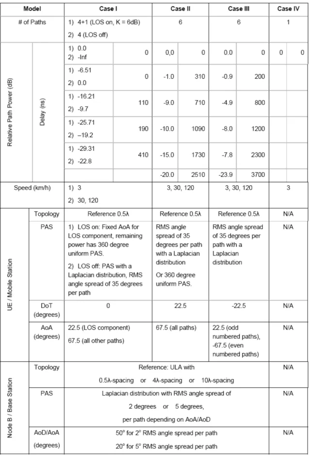
In [8], the spatial channel models for link level and system level simulations are

defined. Link level simulations will not be used to compare performance of different

algorithms. Rather, they will be used only for calibration, which is the comparison of

performance results from different implementations of a given algorithm. Table 2-1

summarizes the physical parameters to be used for link level modeling. The MIMO

channel matrix generation method of the link level model is similar to that described in

(42)

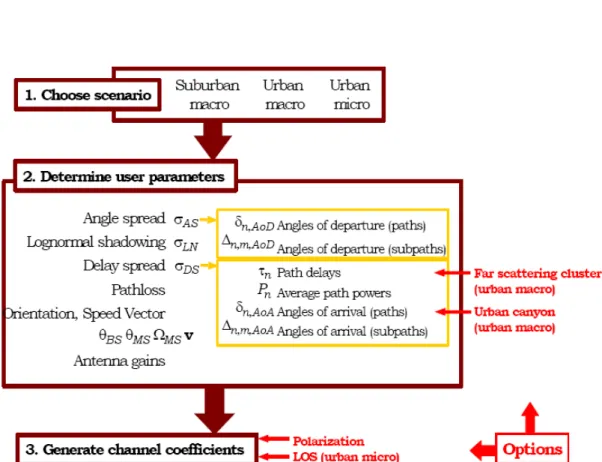
As opposed to link simulations which simply consider a single BS transmitting to a

single MS, the system simulations typically consist of multiple cells/sectors, BSs, and MSs.

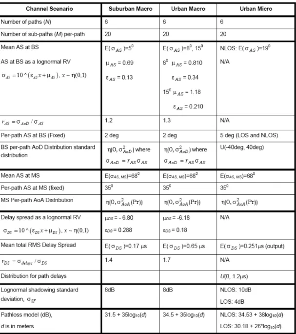
Fig. 2-6 shows a roadmap for generating the channel coefficients. It defines three

environments (suburban macro, urban macro, and urban micro) where urban micro is

differentiated in line-of-sight (LOS) and non-LOS (NLOS) propagations. Detailed model

parameters are listed in Table 2-2. In each environment, the number of paths is equal to 6.

Each path is further composed of 20 spatially separated sub-paths to produce a Rayleigh

fading envelope. The main characteristics of the model include a narrow angle spread (AS)

per-path, with specific base station angle of departure (AoD) and mobile station angle of

arrival (AoA) models. The large-scale behaviors, described by the composite AS, DS and

shadow fading (SF), are simultaneously correlated in the log-normal domain to produce the

expected channel characteristics for each realization of the channel. Path powers, path

delays, and angular properties for both sides of the link are modeled as random variables

defined through probability density functions (PDFs) and cross-correlations.

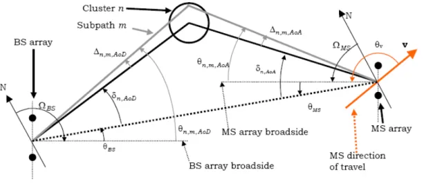
For an S element linear BS array and a U element linear MS array, the channel

coefficients for one of N multipath components are given by a U-by-S matrix of complex

amplitudes. Denote the channel matrix for the nth multipath component (n = 1,…,N) as

) (

(43)

(

)

(

[

(

)

]

)

(

)

(

)

(

)

(

)

∑ = ⎟⎟ ⎟ ⎟ ⎟ ⎟ ⎠ ⎞ ⎜⎜ ⎜ ⎜ ⎜ ⎜ ⎝ ⎛ − × × Φ + = M m v AoA m n AoA m n u AoA m n MS m n AoD m n s AoD m n BS SF n n s u t jk jkd G kd j G M P t h 1 θ θ θ θ θ θ σ , , , , , , , , , , , , , cos v exp sin exp sin exp ) ( (2-25)

where the angular parameters are shown in Fig. 2-7.

The 3GPP SCME is an extension to the SCM for bandwidths up to 20 MHz. In 3GPP

SCME, the 20 sub-paths of SCM are split into 3 subsets, denoted as mid-paths, which are

moved to different delays relative to the original path as shown in Fig. 2-8. The delays and

powers of these 3 mid-paths are predetermined by an exponential power decay function

with 10-ns delay spread. To keep the fading distribution close to Rayleigh, a mid-path is

lumped of 4 or more sub-paths. The mid-path ASs (ASi where i is the mid-path index) are

optimized such that the deviation from the path AS (ASn where n is the path index), i.e. the

AS of all mid-paths combined, is minimized. The delays and the corresponding sub-paths

(44)

(45)

(46)

Table 2-3 Sub-paths to mid-paths assignment and resulting angle spread in 3GPP SCME 1.0247 13, 14, 15, 16 25 ns 4 (of 20) 3 1.0056 9, 10, 11, 12, 17, 18 12.5 ns 6 (of 20) 2 0.9865 1, 2, 3, 4, 5, 6, 7, 8, 19, 20 0 10 (of 20) 1 As_i/ AS_n Sub-paths Delay Number of sub-paths Mid-path 1.0247 13, 14, 15, 16 25 ns 4 (of 20) 3 1.0056 9, 10, 11, 12, 17, 18 12.5 ns 6 (of 20) 2 0.9865 1, 2, 3, 4, 5, 6, 7, 8, 19, 20 0 10 (of 20) 1 As_i/ AS_n Sub-paths Delay Number of sub-paths Mid-path

(47)

Fig. 2-7 The illustration of multipath angle parameters at BS and MS sides.

Excess delay

Power

Path 4: composed of 20 zero-delay, spatially separated sub-paths

3 mid-paths with different relative delays

SCM: 6-path representation SCME: 6*3-path representation

Excess delay

Power

Path 4: composed of 20 zero-delay, spatially separated sub-paths

3 mid-paths with different relative delays

SCM: 6-path representation SCME: 6*3-path representation SCM: 6-path representation SCME: 6*3-path representation

(48)

Chapter 3 Measurement and Modeling

of Wideband SISO Channels

In this chapter, first our proposed method for wideband multipath model parameters estimation is described. We validate this method with extensive measurement data. The measurement setup and environments and the validation results are presented.

(49)

3.1 Introduction

In order to realize the B3G systems, a thorough understanding of the time dispersion

characteristics of radio multipath propagation channels is required. In high-speed wireless

data transmission, severe frequency-selective fading of multipath channel causes

inter-symbol interference (ISI) and leads to a significant problem for the systems. To solve

the problem, modeling of multipath time-of-arrival (TOA), particular on the

multipath-clustering phenomenon, is a fundamental and important work.

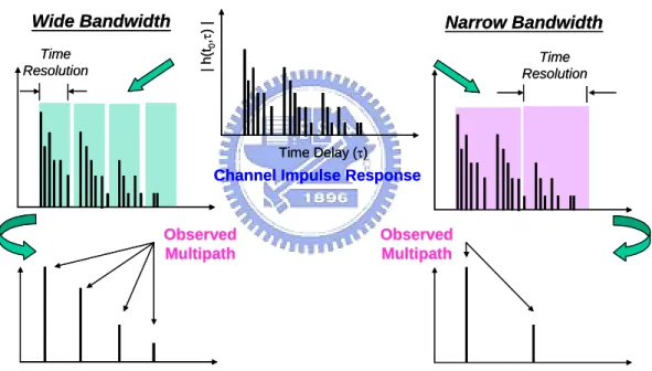
Although there are many researches focused on the exploration or modeling of

multipath-clustering phenomenon, few researches focused on the effect of signal

bandwidth on observed multipath-clustering so far. As shown in Fig. 3-1, it is easily

understood that in the observation of multipath-clustering of a radio channel using a

band-limited signal, the result is mainly affected by the signal resolution, which is the

reciprocal of the signal bandwidth. In this paper, based on the ∆-K model, newly formulas

are derived to describe the relationships between the observed TOA model parameters of

narrowband signals and those of wideband signals. Through this approach, effect of signal

bandwidth on the observable multipath-clustering is explored. Furthermore, to completely

characterize the time dispersion characteristics of the channel, a model using power ratio,

(50)

and amplitude fading is proposed. Formulas to relate these model parameters of a

wideband signal to those of a narrowband signal are also derived. Here, the model

parameter estimation methods have been extensively validated by comparing the computed

channel parameters with the ones extracted from the measured channel responses of 1.95

GHz and 2.44 GHz broadband radios in metropolitan and suburban areas, and of 3-5 GHz

UWB signals in indoors.

Time Delay (τ)

| h

(t0

,τ

) |

Channel Impulse Response Time

Resolution _ResolutionTime

Observed Multipath

Wide Bandwidth Narrow Bandwidth

Time Delay (τ)

| h

(t0

,τ

) |

Channel Impulse Response Time

Resolution _ResolutionTime

Observed Multipath

Wide Bandwidth Narrow Bandwidth

Fig. 3-1 A diagram for bandwidth effect on the observed multipath propagation channels.

3.2 A novel method for wideband model parameter estimation

To explore bandwidth dependency of the model parameters, which include the

clustering parameter, formulas to describe the relationships between observed model

(51)

model is adopted to characterize the multipath-clustering. It is noted that the bandwidth of

the wideband signal is confined to be n times of the narrowband signal’s, where n is a

positive integer. For convenience, the parameters with a subscript f or F correspond to

those of bandwidth f or F, respectively, where F=n⋅f.

3.2.1 Bandwidth on observable multipath-clustering

A. Formulas for wideband to narrowband

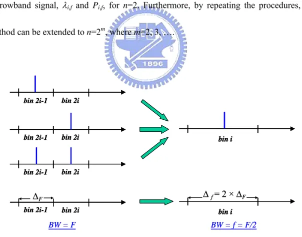
Since a bin width is inversely proportional to its signal bandwidth, ∆f is equal to n⋅∆F,

where ∆f and ∆F are the bin widths of the systems with signal bandwidths f and F,

respectively. Therefore, when a received path occurs at bin i of a signal with bandwidth f,

the path should arrive at one or more of the bins covering from the (n⋅i-n+1)th_{bin to the}

(n⋅i)th_{bin, for the signal with bandwidth F, which is due to the increase of time resolution}

interval. Fig. 3-2 shows an example of n=2.

With the above analysis, λi,f and Pi,f are derived in terms of λj,F and Pj,F by (3-1) and

(3-2), respectively. ) 1 1 1 A r F n r f i, ( + , = ∏ − − = λ λ (3-1) where A= n⋅i-n.

(52)

(

)

(

)

⎪ ⎪ ⎪ ⎪ ⎩ ⎪⎪ ⎪ ⎪ ⎨ ⎧ ⎪⎩ ⎪ ⎨ ⎧ ≥ ⎪⎭ ⎪ ⎬ ⎫ ⎥ ⎦ ⎤ ⎢ ⎣ ⎡ − + − + = − + = ∑ ∏ = + = + − + + + + + + 3 ) 1 1 2 1 3 3 1 2 1 1 2 1 1 n P P n P P P n r A s F r s F r A F A F A F A F A F A F A f i , ( , , , , , , , , , , λ λ λ λ (3-2)

Substituting λi,f and Pi,f into (2-6), ki,f is obtained. Here, let n=2, the analytical

relationship between ki,f and k2⋅i-1,F is found and written as

(

)

(

)

_[

(

₍

)

₎

_]

(

)

[

]

(

)

[

i- ,F i- ,F i- ,F

]

,F i-,F i-,F i-,F i-,F i-i,F ,F i-i,F i,F ,F i-F i f i P P P P k k k 3 2 2 2 3 2 3 2 2 2 3 2 2 2 2 2 2 1 2 2 2 1 2 1 2 1 1 1 1 1 1 ⋅ − ⋅ + ⋅ ⋅ − ⋅ + ⋅ ⋅ ⋅ ⋅ ⋅ ⋅ ⋅ − ⋅ + ⋅ ⋅ − ⋅ ⋅ − ⋅ = − ₋ λ λ λ λ λ λ λ λ , , (3-3)

On the right-hand side of (3-3), magnitudes of the second and third factors are in the

range of 0 to 1. From (3-3), it is found that ki,f is smaller than k2⋅i-1,F if k2⋅i-1,F > 1. It means

that wider bandwidth signal observes stronger multipath-clustering phenomenon. It is

noted that k2⋅i-1,F ≅ k2⋅i,F, which is found from measurement data and is shown in Section

3-3.

B. Formulas for narrowband to wideband

With (3-1) and (3-2), the observed model parameters of a narrowband signal cannot

(53)

condition is needed to determine three unknown parameters, λ2⋅i-1,F, λ2⋅i,F and P2⋅i-1,F with

those of bandwidth f, λi,f and Pi, f. Here, the condition is given by assuming λ2⋅i-1,F =λ2⋅i,F,

i.e., the path arrival rates of two neighboring bins are equal. It is because that for both

outdoor broadband and indoor UWB radio channels, multipath excess delay time is much

larger than the time resolution (bin width). Based on this assumption, λ2⋅i-1,F and λ2⋅i,F are

solved from (3-1)

2 1

2i ,F λ i,F 1 1 λi,f

λ _⋅ ₋ = _⋅ = − − (3-4)

However, our assumption may lead to underestimate λ2⋅i-1,F and overestimate λ2⋅i,F

since the path arrival rate decreased asymptotically with bin number. To reduce the

estimation errors, λ2⋅i-1,F and λ2⋅i,F from (3-4) are modified using the interpolation method

and are given by (3-5a) and (3-5b), respectively

(

)

⎭ ⎬ ⎫ ⎩ ⎨ ⎧ ⎥⎦ ⎤ ⎢⎣ ⎡ ₊ _⋅ ₋ = _⋅ ₋ _⋅ ₋ _⋅ ₊ − ⋅ 1 2 1 2 1 2 1 2i ,F min 1, λ i ,F ₄1 λ i ,F λ i ,F λ (3-5a)

(

2 1 2 1

)

1 2 2⋅i,F =λ ⋅i− ,F −1₄⋅ λ ⋅i− ,F −λ ⋅i+ ,F λ (3-5b)

It is noted that λ2⋅i-1,F and λ2⋅i+1,F on the right-hand side of (3-5a) and (3-5b) are

(54)

(

2

) (

2

)

1

2i F P_i _f i F 1 i F

P _⋅ ₋ _, = _, −λ _⋅ _, −λ _⋅_, (3-6a)

P2⋅i,F is computed by averaging its neighboring points and is given by (3-6b)

(

₂ ₁ ₂ ₁

)

2 2iF P i F P i F

P_⋅_, = _⋅₋ _, + _⋅₊ _, (3-6b)

Substituting λj,F and Pj,F into (2-6), kj,F is obtained. Through the above approaches, the

model parameters of a wideband signal, λj,F, Pj,F and kj,F, are determined by those of a

narrowband signal, λi,f and Pi,f, for n=2. Furthermore, by repeating the procedures, this

method can be extended to n=2m_{, where m=2, 3, ….}

bin 2i-1 bin 2i

bin i

bin 2i-1 bin 2i _{bin i}

BW = F BW = f = F/2

∆F ∆f= 2 ×∆F

bin 2i-1 bin 2i

bin i bin i bin i

bin 2i-1 bin 2i _{bin i}

bin 2i-1 bin 2i _{bin i}_{bin i}

BW = F BW = f = F/2

∆F ∆f= 2 ×∆F

(55)

3.2.2 Bandwidth on multipath power decay and amplitude fading

To completely characterize the time dispersion characteristics of the channel, effects

of bandwidth on multipath averaged power decay and amplitude fading are analyzed as

follows.

A. A statistical model for multipath averaged power decay and amplitude fading

In many literatures for broadband and UWB radio channel modeling [34-35], the

small-scale averaged power delay profile (aPDP), g

( )

τ , is modeled by an exponential time

decay function with a stronger first bin and is expressed as

( )

[

(

)

]

( )

_⎥ ⎦ ⎤ ⎢ ⎣ ⎡ Γ − − + = ∑ = i L i i G g τ δ τ γ τ τ δ τ 2 2 1 1 exp (3-7)

where G₁ is the mean power of the first bin, τi is the relative time delay of bin i and is

equal to (i-1)⋅∆, γ is the power ratio that is defined as the ratio of the second bin’s mean

power to the first bin’s mean power, Γ is the exponentially power decay constant and δ is

the Dirac delta function. From our extended measurement data at indoor environments, one

of the examples shown in Fig. 3-3, it is found that this model well describes the measured

aPDP.

(56)

follows a Rician distribution with a large Rician factor and the later bins tend to follow the

Rayleigh statistics (the Rician factor is closed to zero), as shown in Fig. 3-4. It is noted that

measured points no.1-no.12 are in LOS (Line-of-Sight) situations and the rest points are in

NLOS (Non LOS) situations. Details of measurements are described later in Section 3.3.2.

Power ratio

Exponentially power decay

Power ratio

Exponentially power decay

Fig. 3-3 The averaged power delay profile of a 500 MHz-bandwidth UWB signal at an indoor environment and under NLOS condition. The wavy line shows the measured profile. The straight line, which is obtained by a best-fit procedure, represents an exponential decay line.

(57)

Fig. 3-4 Rician factors of the first 15 bins of each measured point at indoor environments with 2-GHz bandwidth are shown. The total numbers of measured points are 24.

B. Formulas for wideband to narrowband

For an uncorrelated scattered radio propagation channel [36], bins’ amplitudes are

distributed independently of one another, and the averaged bin power is calculated by the

power sum of multipath in a bin. For example, averaged power sum of two successive bins

for bandwidth F is equal to the averaged power of the corresponding bin for bandwidth f

頻寬-空間-極化於寬頻多輸入多輸出無線電通道影響之研究

國 立 交 通 大 學

電信工程學系

博 士 論 文

頻寬-空間-極化於寬頻多輸入多輸出無線電

通道影響之研究

Effects of Bandwidth-Space-Polarization on

UWB/Wideband Multiple-Input Multiple-Output

Channels

研 究 生：張維儒

指導教授：唐震寰 博士

頻寬-空間-極化於寬頻多輸入多輸出無線電

通道影響之研究

Effects of Bandwidth-Space-Polarization on

UWB/Wideband Multiple-Input

Multiple-Output Channels

研究生：張維儒

Student:

Wei-Ju

Chang

指導教授：唐震寰 博士 Advisor:

Dr.

Jenn-Hwan

Tarng

國立交通大學

電信工程學系

博士論文

A Dissertation

Submitted to Institute of Communication Engineering

College of Electrical and Computer Engineering

National Chiao Tung University

in Partial Fulfillment of the Requirements

for the Degree of Doctor of Philosophy

in

Communication Engineering

Hsinchu, Taiwan

頻寬-空間-極化於寬頻多輸入多輸出無線電

通道影響之研究

研究生：張維儒 指導教授：唐震寰 博士

國立交通大學電信工程學系

中文摘要

Effects of Bandwidth-Space-Polarization on

UWB/Wideband Multiple-Input

Multiple-Output Channels

Student:

Wei-Ju

Chang Advisor:

Dr.

Jenn-Hwan

Tarng

Institute of Communication Engineering

National Chiao Tung University

Abstract

誌

謝

Contents

List of Tables

List of Figures

Abbreviations

Chapter 1 Introduction

1.1 Motivation and Contributions

1.2 Thesis Overview

Chapter 2 Overview of Channel

Models for B3G Systems

2.1 Introduction

( )

(

)

(

)

(

) (

) (

)

( )

( )

( )

( )

( )

( )

國立交通大學

博士論文

研究生：張維儒

指導教授：唐震寰博士

指導教授：唐震寰博士 Advisor:

研究生：張維儒指導教授：唐震寰博士