生物系統內分子交互作用及生化路徑之大規模分析---子計畫二:智慧型最佳化方法用於基因網路的重建與分析(III)

(1)

行政院國家科學委員會專題研究計畫成果報告

生物系統內分子交互作用及生化路徑之大規模分析--(子計

畫二)智慧型最佳化方法用於基因網路的重建與分析(3/3)

研究成果報告(完整版)

計畫類別：整合型計畫編號： NSC 99-2627-B-009-002- 執行期間： 99 年 08 月 01 日至 100 年 07 月 31 日執行單位：國立交通大學生物科技學系（所）計畫主持人：何信瑩計畫參與人員：碩士級-專任助理人員：劉品辰學士級-專任助理人員：宋禹碩士班研究生-兼任助理人員：張孝邦碩士班研究生-兼任助理人員：林意哲碩士班研究生-兼任助理人員：林玉祥碩士班研究生-兼任助理人員：高德芬博士班研究生-兼任助理人員：陳義雄博士班研究生-兼任助理人員：高國慶博士班研究生-兼任助理人員：蔡明儒處理方式：本計畫涉及專利或其他智慧財產權，2 年後可公開查詢

中華民國 100 年 10 月 31 日

(2)

摘要

推論基因調控網路(Gene Regulatory Network)來發現一些重要的調控關係，在後基因體時代扮演很重要的角色，尤其在分子生物學、生物化學、生化工程學以及製藥學上更是舉足輕重。本子計畫依據不同需求下之基因調控網路模型，將調控網路的建立變成大型的參數最佳化問題。針對不同模型的基因調控網路，本計畫提出最佳化方法依模型推論基因調控網路來建立網路單元的調控關係: (1)含所有調控關係：調控因子(Transcription factors, TFs)對基因，TFs 對 TFs 及基因對 TFs 之調控網路重建，在考量實際生物微陣列資料樣本數太少和雜訊，以 S-system 模型發展改良方法 iAEA，來克服無限多解導致網路無法鎖定的問題。(2)以目標基因為出發點，針對調控其表現量之 TFs 的調控網路重建，以

Network Component Analysis (NCA)為主軸，提出的智慧型最佳化方法 GRNet。兩者除了使用基因表現量資料外，並透過文獻已知的基因調控關係來重建網路。在第一年執行期間，配合子計畫三的基因調控資料庫，進行模擬實驗，發展 iTEAP 及 GRNet+建立有效且能夠不受實驗雜訊影響的網路重建方法，並證實核心演算法在於不同需求下的網路重建，都能有效地建立可供參考的調控網路。接著針對不同模型的基因調控網路，第二年延伸第一年提出之解決實際生物微陣列資料樣本數過少，以及不受實驗雜訊影響的網路重建方法，進行改良與整合。第二年完成整合子計畫三之生化路徑與基因調控資料庫，配合繪圖運算單元(GPU)叢集，進行網路重建平台(Gene Network Platform, GNP)

建置。透過使用GPU 提昇平台運算效能近十倍，並針對大腸桿菌之調控網路進行重建，以視覺化方式

呈現並進行分析。

第三年根據模擬與實際資料分析結果，持續改良核心演算法並發展 Intelligent Adaptive-encoding

Evolutionary Algorithm (iAEA)有效解決雜訊與無限多組解的問題，並與子計畫合作對於厭氧條件轉至

有氧條件下之大腸桿菌網路進行網路重建預測，發現調控因子CRP, Fnr 對於 fumC 的調控關係，並於基因晶片實驗中獲得證實，該調控關係並未發表於最新的RegulonDB 中。本三年計畫衍生成果包括發展多項生物資訊預測的演算法及其應用，研究成果豐碩。合計已發表相關期刊論文 13 篇，及已投稿和複審中 3 篇期刊論文，及已發表 14 篇國外會議論文。並將該核心建模方法「智慧型演化式演算法於數學建模與預測的最佳化機制」套件模組化，便於日後進行技術轉移到業界應用。關鍵詞：演化式計算、直交退火演算法、基因調控網路、網路分析模型、S-system 基因網路模型、統一運算架構、繪圖運算單元

(3)

Abstract

Inference of gene regulatory networks (GRNs) plays an important role in molecular biology, biochemistry, bioengineering, and pharmaceutics in the post genomic research. According to different models for GRNs with transcription factor (TF) or not, reconstructing GRNs from mathematical models can be formulated as large-scale parameter optimization problems. The project proposes evolutionary optimization algorithms to obtain near-optimal solutions to the problems of reconstructing GRNs. (1) GRNs with all regulations: In reconstruction of GRNs, the regulations contain TF-gene, TF-TF, and gent-TF. Because of it’s degrees increase and make this reconstruction problem more complex and inconsistent of possible solutions. To cope with noise and insufficient data problems, we propose iAEA based on S-System model to efficiently reconstruct GRNs; (2) GRNs considering interested genes with TF-gene regulations: The well-known method as Network Component Analysis (NCA) is used, we propose GRNet based on Intelligent Evolutionary Algorithm (IEA) and NCA model. In addition to time-series data of gene expression, the connectivity data between TF and gene is used for both methods to infer GRNs.

In the first year, we cooperate with regulatory database in sub-project in this integrated research project for our simulation to develop efficient and robust methods: iTEAP and GRNet+ to cope with noise to reconstruct GRNs. The stabilities of predicted GRNs are achieved.

We also cooperate with regulatory database in the sub-project III in this integrated research project for Gene Network Platform (GNP). The GNP with graphics process unit (GPU) clusters achieve about 10 times faster to reconstruct GRNs. The regulatory network of Escherichia coli is also optimized with GNP and friendly charts are used for visualization and analysis.

In the last year, we improve our core algorithms continuously with previous experiments and propose an Intelligent Adaptive-encoding Evolutionary Algorithm (iAEA) to cope with noise and inconsistent solutions with domain knowledge as GRNet. Biological experiments of E. coli during transition from anaerobic to aerobic conditions are used with GNP to predicted unknown regulations that are not found in latest version of the database RegulonDB. The prediction of GNP is proved from RT-PCR experiments that CRP activates fumC and Fnr inhibits fumC during the transition.

The extended achievements of this three-year project are good, including several bioinformatics prediction algorithms and their applications. There are totally 13 published journal papers and 3 submitted ones, and 14 international conference papers. We package the core modelling method “Intelligent Evolutionary Algorithm for the Optimization Mechanism of Mathematical Modeling and Prediction” for transferring the related technologies to industry for various applications in future.

Keywords: Evolutionary Computation, Orthogonal Simulated Annealing, Gene Regulatory Network, Network Component Analysis, S-System, Compute Unified Device Architecture, Graphics Processing Unit

(4)

List of Figures

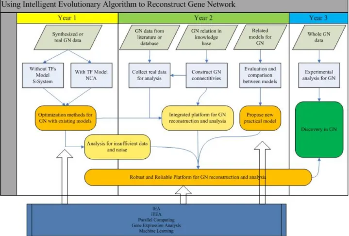
FIGURE 0.1: ROADMAP AND RELATED TASKS TO RECONSTRUCT GRNS. THE PARALLELOGRAMS IN GREY ARE EXISTED DATA OR KNOWLEDGE. THE RECTANGLE IN BLUE INDICATES THE IMPROVEMENTS WE APPLIED OR EVALUATE FROM CURRENT RESULTS OR RESEARCHES. THE ROUND-‐

RECTANGLE IN ORANGE OR GREEN IS FINAL GOALS OR FINDING. ... 1

FIGURE 2.1: ILLUSTRATION OF GENE REGULATORY NETWORK[25] ... 3

FIGURE 3.1: CHROMOSOME REPRESENTATION. ... 7

FIGURE 3.2: THE ARCHITECTURE OF GNP FOR RECONSTRUCTING GENE NETWORK: THE YELLOW, GREEN, AND BLUE AREAS REPRESENT THE INVOLVED PARTS FOR FIRST TO THIRD YEAR IN OUR SUB-‐PROJECT. THE RED AREA IS DONE BY OTHER PROJECT. ... 9

FIGURE 4.1: COMPARISONS OF LSE BETWEEN GRNET AND NCAR. ... 10

FIGURE 4.2: COMPARISONS OF CSDIFF BETWEEN GRNET AND NCAR. ... 11

FIGURE 4.3: COMPARISON OF LSE BETWEEN NCAR AND GRNET FOR 10 SILICO-‐DATASETS ... 12

FIGURE 4.4: COMPARISON OF CS CONFLICTS BETWEEN NCAR AND GRNET FOR 10 SILICO-‐DATASETS ... 12

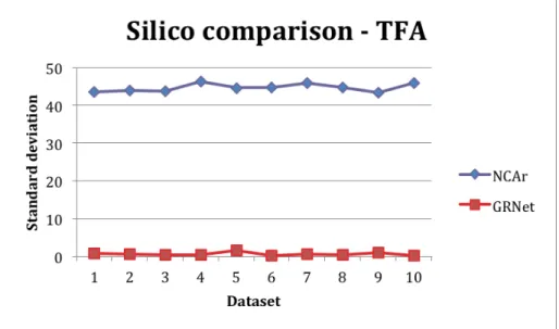
FIGURE 4.5: COMPARISON OF STANDARD DEVIATION TO REAL TF ACTIVITIES BETWEEN NCAR AND GRNET FOR 10 SILICO-‐DATASETS ... 12

FIGURE 4.6: SPEEDUP WITH CUDA ARCHITECTURE. ... 13

FIGURE 4.7: TIME COURSE OF TF ACTIVITIES FROM NCA[1]. ... 14

FIGURE 4.8: TF ACTIVITIES DEDUCED FROM TGRNET. ... 15

FIGURE 4.9: COMPARISONS OF CAMP CONCENTRATION DURING GLUCOSE TO ACETATE TRANSITION ARE MADE BETWEEN EXPERIMENT AND TGRNET. LEFT SIDE IS OBSERVED FROM BIOLOGICAL EXPERIMENT[37]. RIGHT SIZE IS THE TF ACTIVITIES FROM TGRNET. ... 15

FIGURE 4.10: FLOWCHART TO USE GNP FOR RECONSTRUCTING GRNS. ORANGE RECTANGLES ARE ACTIONS USER NEED TO HANDLE. ... 16

FIGURE 4.11: E. COLI (FROM KAO’S DATA)GRNS PREDICTED BY GNP. ... 16

FIGURE 4.12: THE EXPERSSION PROFILES FOR BOTH INVOLVED GENES AND TFS. ... 17

FIGURE 4.13: CONNECTIVITY DATA OF E. COLI DATA IS SHOWN. THERE ARE 6 REGULATIONS ARE MARK AS UNKNOWN WITH SYMBOL X. ... 17

FIGURE 4.14: EXPRESSION PROFILES WITH DIFFERENT PRIORI KNOWLEDGE IN [CS]. ... 18

(6)

List of Tables

TABLE 4.1: SILICO AND EXPERIMENTAL RESULTS COMPARISON ... 11

TABLE 4.2: COMPARISON BETWEEN GRNET, REGULONDB, AND TSENG’S LAB IN 30 RUNS ... 18

TABLE 4.3: COMPARISON BETWEEN IAEA, REGULONDB, AND TSENG’S LAB IN 50 RUNS ... 18

(7)

0. Introductions

The inference of biochemical networks, such as gene regulatory networks, protein-protein interaction networks, and metabolic pathway networks, from time-course data is one of the main challenges in systems biology. The ultimate goal of inferred modeling is to obtain expressions that quantitatively understand every detail and principle of biological systems. To solve the large-scale and complex reversing engineering problem, the sub-project would propose intelligent optimization algorithms combined with biological domain knowledge for coping with noise and insufficient data problems of practical applications. The proposed methods will be verified using synthesized and real data. In this sub-project, we propose two efficient methods for inferring various biochemical networks depends on needs and integrate them with biological data warehouse to build a user-friendly platform, which can also benefit the other sub-projects.

Figure 0.1: Roadmap and related tasks to reconstruct GRNs. The parallelograms in grey are existed data or knowledge. The rectangle in blue indicates the improvements we applied or evaluate from current results or

researches. The round- rectangle in orange or green is final goals or finding.

In the first year, IEA was used to develop effective algorithms for various mathematical models. As mentioned above, we choose two widely used models: S-System and Network Component Analysis (NCA) for gene network reconstruction considering the details of regulations involved. The major goal is to develop optimization methods for real experimental data while the performance is evaluated using synthesized data. We take the problems of insufficient data and measured noise into consideration for modeling from experimental data of gene network before we start to integrate the gene network platform (GNP). We applied

(8)

statistical and mathematical methods to help us to solve this problem and extend the power of IEA with successful experiences in gene expression analysis.

Most of the existing models come with limitations [1]. For example, cooperative mechanism and combinatorial control in gene regulation of gene and TFs occurs in many cases [2] . NCA only implies gene was regulated by TFs. Comparison and evaluation in models proposed by other researchers will be done in the second year first. Then, we aim to establish a GNP with anti-noise and efficient methods that need less data proposed in the first year. Using Biomolecular Interaction Data Warehouse proposed in sub-project 3 to obtain connectivity of gene-gene or gene-TFs as optimization criteria for initial solutions and try to avoid from violating known regulations.

At the last year, as success of GNP we start our case study for analysis of reconstructed gene regulatory networks. We focus on E. coli first due to the availabilities and integrity of experimental data for the first two years. In this year, biological experiments will help us to verify our results of computational simulation, which was done by the collaboration of all PIs and co-PIs of this integrated project.

1. Motivations

Reconstructing gene regulatory networks (GRNs) plays an important role in many research disciplines such as molecular biology, biochemistry, bioengineering, and pharmaceutics. In order to help biologists to study and analyze specific biological mechanisms, benefit pharmacy, and disease therapy from a systematic viewpoint, it is necessary to clarify the regulatory relationship of genes and transcription factors. Recently, we have proposed efficient evolutionary algorithms for identifying dynamic pathways from time-course gene expression profiles. The methods iTEA and GRNet are shown to be efficient for synthesized data sets. The objective of this sub-project is to develop various problem-specific intelligent optimization algorithms as well as an integrated platform for reconstructing biochemical networks such as gene regulatory networks and figure out the regulatory relationship between genes. With the help of the structural information from sub-project 1 and knowledge of biological database from sub-project 3, the feasible range of parameters is restricted and makes the proposed methods to acquire accurate regulatory relationship. By the cross validation of related literatures, biological experiments, simulation results, and biological knowledge from sub-project 3, the reliable regulatory relationships can be further confirmed. Furthermore, additional analysis of the problem caused by insufficient data and noise of experiments data is conducted to propose an adding-noisy-duplicate technique to solve the ill conditioned and system uncertainty problems, which can therefore reduce the required experimental resource. This analysis is expected to provide the information about a minimal number of gene expression profiles for reconstructing a reliable gene network mode. In addition to silicon simulation, an overview of whole genes for species may find something new and biological experiments would be applied to verify the findings.

2. Related works

The inference of biochemical networks would focus on gene networks first. Several models had been proposed to reconstruct complex gene networks, and used for understanding the activation, inhibition, and transcriptional strength between genes and transcription factors. In general, gene network is reconstructed by

(9)

gene expression data measured by Real-Time Polymerase Chain Reaction (RT-PCR). The numerous mathematical algorithms and models were proposed to describe biochemical networks include[3]: the Boolean network model [4, 5] the Bayesian network [6-9], and the differential model or S-system model [3, 10-24]. In Boolean network models, gene expression levels can refer to two situations: true or false. The Bayesian network model is able to deal with linear, nonlinear, and combinatorial problems and is also used to infer genetic networks. However, similarly to Boolean networks, it suffers from the same dilemma and is only applicable to acyclic structures. The most popular model is referred to as NCA and S-system model, which have been applied to reconstruct various fundamental gene regulatory networks in many researches.

Figure 2.1: Illustration of Gene Regulatory Network[25]

2.1 Reconstruct GRNs with all regulations: S-system model

The S-system model has been considered suitable to characterize non-linear regulatory network systems and is able to reflect gene expression continual variation dynamics. It is a set of non-linear differential equations of the following form:

1 1

,

ij ij N N g h i i j i j j j

dX

X

dt

=

α

∏

₌

−

β

∏

₌ i=1, …, N, (1)

Where Xi represents the expression level of gene i and N is the number of genes in a genetic network. αi

and βi are rate constants, which indicate the direction of mass flow and must be positive. gij and hij are kinetic

orders which reflect the intensity of interaction from gene j to i. For inferring an S-system model, it is

necessary to estimate all the 2N(N+1) S-system parameters (αi, βi, gij, hij) from experimental time-series data

of gene expression. However, reconstructing large-scale (N > 50) gene regulatory networks is more important than reconstructing small-scale gene regulatory networks in biological researches. Because there involve many genes in a biological function process.

Therefore, reconstructing large-scale gene regulatory networks using S-system model became large number parameter simultaneously optimize problems. Many researchers proposed diverse methods using numerical methods such as steady-state analysis[26] and evolutionary algorithms[3, 13, 17, 20, 23, 24, 27] to solve the optimization problem. The genetic algorithm (GA) plays an important role in solving the optimization problem of dynamic modeling of gene regulatory network using the S-system model.

(10)

2.2 Reconstruct GRNs with TFs-genes regulations: Network Component Analysis

Network component analysis (NCA) is known as a model-based decomposition method for GRN to deduce information of TF activities and control strength (CS) of TF-gene connectivity network. Gene expression data is real microarray data and TF-gene connectivity is collected from literature or public database. This decomposition matrix can be solved by singular value decomposition [28-30]. Conventional approaches, such as PCA and ICA, typically seek a matrix of [CS] such that the resulting reconstructed signal matrix [TFA] satisfies orthogonality or independence criteria, respectively [1, 31, 32]. To ensure unique solutions of matrix decomposition, NCA requires some criteria to be satisfied. In practice, some information, such as relationship of TF-gene regulation or potential unknown regulation, is ignored to prevent from the uncertainty of matrix computation. Due to criteria used for matrix reduction, up or down regulation may be incorrect in some case. Therefore, biologists need some prior knowledge to determine if invert observed TF activities or not. In addition to that, the predicted TFs are not equal to competent TFs (a.k.a. TFAs) that have ability to bind promoter, so the amount of TFAs should identify to match real biological system. However, TFAs are still hard to determine through experiments approach thus NCA is still a good model to determine TFAs [33].

NCA can uncover hidden regulatory signals from outputs of networked systems, when only a partial knowledge of the underlying network topology is available [1]. The author implements a Matlab package for biologist to study regulations beyond interesting gene regulatory network. The NCA adopts alternative method with QR factorization to solve minimizing least square problem. It’s not very stable depends on initial value of TF-gene connectivity [25, 34, 35] and may exist multiple local minima [33, 34]. The subsequently developed NCAr algorithm with Tikhonov regularization can help solve the first issue but cannot completely handle the second one [25]. The total number of source signal components was limited to the total number of experiments rather than the total number of biological regulators in NCA. In most case, biologist would like to analyze regulatory network as many important TF as possible to prevent from loss of regulation in regulatory network. However, networks that have less transcriptome data points than the number of regulators are common. There is an enhanced release to replace these constraints with the TFs regulating each gene must be linearly independent in the available experiments [35]. NCA package would take lots of time while applying to large regulatory network, one make an enhanced FastNCA to reduce the time cost NCA needed [34] . They claim FastNCA is more accurate and is not sensitive to the correlation among the input signals than that of NCAr and comparable to that of properly converged NCA. Although NCA model comes with some short comes, NCA is one of feasible model that can infer a conceptual GRNs [36] [38], or reveal new TF-gene regulations [39].

3. Methods

These proposed models describe the networks through their inner parameters. When the scale of network is increased, the number of parameters that need to be optimized is also significantly increased. An effective computational gene network model should realize the observed dynamic gene expression and reflect the regulatory relationship between genes. For this reason, gene network is often reconstructed from the observed gene expression profiles. To describe the network appropriately, it is inevitable to optimize the inner parameters of model through the observed data. Because of limited resource and time, the available data is too

(11)

few to prevent model uncertainty. Optimization methods will be proposed to solve the problem of model uncertainty when modeling gene networks from insufficient data and noise.

3.1 Efficient and robust method: GRNet

NCA is known as a useful analysis tool for GRNs. The main concept of NCA is shown as Figure 1.2. The gene expression level is determined from transcription factor (TF) activities and control strength (CS) for specific gene. The linear model of NCA is shown in equation (2):

E= CS ⋅TFA + Γ (2)

where E is the expression profiles of genes that measured by DNA microarray. CS is composed of the regulation between TFs and genes. TFA represents activities of associated transcription factors. NCA decomposes data matrix E into CS and TFA by minimizing Γ under the constraints that the network structure or the non-zero pattern of the matrix CS is conserved [1]. E is the known M × T matrix that contains M genes and T time points under specific condition. CS is the unknown M × N matrix considers N transcription factors regulate to M genes. Corresponding to E and CS, TFA shows that activities of N transcription factors at T time points.

11 1 11 1 11 1 1 1 1 n o n m mn m mo o on E E CS CS TFA TFA E E CS CS TFA TFA ⎛ ⎞ ⎛ ⎞ ⎛ ⎞ ⎜ ⎟ ⎜₌ ⎟ ⎜_× ⎟ ⎜ ⎟ ⎜ ⎟ ⎜ ⎟ ⎜ ⎟ ⎜ ⎟ ⎜ ⎟ ⎝ ⎠ ⎝ ⎠ ⎝ ⎠ K K K M O M M O M M O M L L L (3) 3.1.1 Evaluations of GRNet

An efficient and robust evolutionary method GRNet is investigated to reconstruct GRNs from gene expression data and known TF-gene connectivity. A mathematical model of NCA is defined as equation (3). We aim to optimize both signs and magnitudes of TF activities and CS while considering noisy gene expression data. The initial values of CS are known regulation between gene and TF from public literature and database and in the set of [1, -1, 0] to represent up-regulation, down-regulation, and no regulation respectively. The model reconstruction is formulated as an optimization problem where least square error (LSE) between the known and estimated expression data is used as an objective function to be minimized. LSE is defined in equation(4). High performance of GRNet arises mainly from an orthogonal simulated annealing algorithm [36] to solve the large-scale optimization problem.

LSE= ( E⎡⎣ ⎤⎦ − cs⎡⎣ ⎤⎦ tfa⎡⎣ ⎤⎦)

2 ₍₄₎

With achievements of the lower LSE, the regulation between TFs and genes should be noticed for better understanding of estimated GRN. An evaluation function is defined in equation(5). We check the signs of final [cs] to [CS] from prior knowledge that demonstrate if TF induce or repress specific gene or not. This information will help us to identify precise TF-gene network structure for unknown or violated information from literature or published database.

(12)

CS_diff = Sign(cs_ij,CS_ij) j=1 T

∑

i=1 M

∑

(5)

However, the regulations in GRNs include TF-gene, TF-TF, and gene-TF in physiological process. In NCA, TFA matrix is defined as activities of TF. In equation(2), the [TFA] is described as activities for standalone TF. Regarding to TFs act in combination on promoter, it’s also an important regulations to control gene expression. Hence, Temporal GRNet (tGRNet) is proposed for more straightforward GRNs. The idea of tGRNet is based on the strength of [CS] should be determined as time goes by. The control strength for each gene can be summarized with TFs, TFs in combination, and even feedback by gene in next time points. This model is extended from NCA and defined as temporal NCA (tNCA). tGRNet implements tNCA to validate the practicability for GRNs.

3.2 Efficient and robust method: iAEA

To effectively reconstruct gene network using S-system model and avoid the problem of model uncertainty, sufficient data for modeling is required. In order to increase the number of data, L sets of additional data are produced by adding k% random Gaussian noises to real experimental data using the following equation,

( )

, , 2 , , 0, pseudo i t l obs i t X =X +N σ , (6)

where Xobs,i,t is experimental observed expression level of gene i at time t, and Xl_{pseudo i t}_{, ,} is the l-th produced

pseudo expression data, N(0, σ2_{) is a normal distributed random number function with zero mean and variance}

σ2_{. Here, σ is assigned as X}

obs,i,t × k%.

The extended optimization method we proposed in the second year (named iTEAP) bases on iTEA to infer the S-system models of genetic networks from a time-series real data set of gene expression profiles using SOS DNA microarray data in E. coli as an example. The algorithm iTEAP generated additionally multiple data sets of gene expression profiles by perturbing the given data set. The results reveal that 1) iTEAP can obtain S-system models with high-quality profiles to best fit the observed profiles; 2) the performance of using multiple data sets is better than that of using a single data set in terms of solution quality, and 3) the effectiveness of iTEAP using a single data set is close to that of iTEA using two real data sets. The obtained model can be validated by biological experiments and known knowledge.

The goal of iAEA, an improved version of iTEA and iTEAP, in GNP is to solve the infinite solutions of the S-system model for efficiently establishing large-scale GRNs by incorporating the domain knowledge of gene regulation into the proposed evolutionary computation method. The novel encoding chromosomes used

the intelligent genetic algorithm.Because of the connectivity of the genetic network has been known to be

sparse, domain knowledge was provided for the encoding chromosome. Let I is a maximum in-degree of the

maximal number of genes that directly affect gene. The iAEA uses a hybrid encoding method that consists of

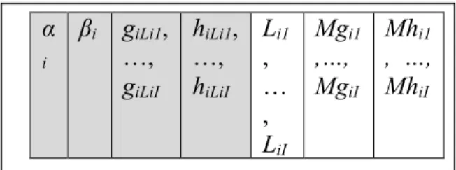
regulation strength, gene number regulated, and binary control parameters in a chromosome. 3.2.1 Chromosome encoding method

The chromosome representation for each gene i, shown in Figure 3.1, consist of three parts: 1) rate

(13)

mass flow. giLij and hiLij are kinetic orders that reflect the intensity of interaction from gene Lij to i, where Lij

belongs to {1, 2, …, N} and j=1,.., I. Mgij is a mask parameter of a positive kinetic order which the value 1

represents the edge of gene Lij to i in the structure of the gene regulatory network is connected. And zero

represents the edge is disconnected. Similarly, Mhij is a mask parameter of a negative kinetic order. Mgij and

Mhij belong to {0,1}. The two sets {αi,βi, giLi1,…, giLiI, hiLi1,…, hiLiI } and {Li1, …, LiI, Mgi1,…, MgiI Mhi1,…,

MhiI } of S-system parameters are real and integer values, respectively. There are 2×I+2 real variables and 3×I

integer variables in our genetic algorithm.

Figure 3.1: Chromosome representation. 3.2.2 iAEA Algorithm

The algorithm for solving subproblems is given as follows:

Step 1:Randomly set the connected state of gene regulation in each subproblem.

Step 2:Initiation: Randomly generate an initial population with Npop feasible individuals of 2×(I+1)

real-valued parameters and 3×I integer-value parameters. Step 3:Evaluation: Evaluate fitness values of all individuals.

Step 4:Selection: Use the simple ranking selection that replaces the worst Ps×Npop individuals with the best

Ps×Npop individuals to form a new population, where Ps is a selection probability. Let Ibest be the best

individual in the population.

Step 5:Crossover: Randomly select Pc×Npop individuals including Ibest, where Pc is a crossover probability. Perform perturbation intelligent crossover operations for all selected pairs of parents.

Step 6:Mutation: Apply the two different mutation operators to real-value and integer-value of the population

using a mutation probability Pm. To prevent the best fitness value from deteriorating, mutation is not

applied to the best individual.

Step 7:Repeat 50 times from step2 to step 6.

Step 8:Selected the fitness of subproblem was solved good enough from the 50 times experiments, then counted the number of gij, and hij.

Step 9: Termination test: If fitness evaluation is achieved in this 50 times experiments, then stop the algorithm. Otherwise, according statistical result from Step 8, set the connected state was fixed or unfixed in each gene, then go to step 2.

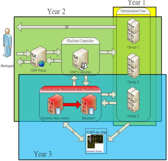
3.3 Integration of gene network platform

The architecture of GNP is shown as Figure 3.2. The optimization core was completed at the first year based on proposed methods for gene networks reconstruction considering with or without transcription factors. The two tasks in this year are integration of biomolecular interaction data warehouse built in sub-project 3 and

α i βi giLi1, …, giLiI hiLi1, …, hiLiI Li1 , … , LiI Mgi1 ,…, MgiI Mhi1 , …, MhiI

(14)

Main components in GNP are described as follows:

l Optimization core: this unit serves as computational core based on proposed methods. Different groups used to share information and balance the computation load. Parallel computation is introduced to optimize gene network based on our previous work “Developing a parallel intelligent optimization system based on evolutionary algorithm for genetic network modeling” (NSC-95-2221-E-009-116). In addition to our achievements, we consider transcription factors in dedicated application of GRNs, insufficient data and experimental noise for modeling in this project.

l GNP portal site: A portal server to provide user-friendly interface for biologists.

l Platform controller: The controller can determine how our system to work. Query from data warehouse or activate optimization core to inference gene network based on information for specific gene network.

l Biomolecular Interaction Data Warehouse: In sub-project 3, a data warehouse of GN was built and up-to-date from latest literature and databases.

GNP allows biologists to select interesting genes to reconstruct their gene network before performing experiments. In Figure 1.2, grey arrow indicates the working flow between components of GNP and the number is execution order when requests come in. GNP portal let them to select species they want in GNP if no more prior knowledge provided. Additional option for TFs, constraints of gene-gene or gene-TF interaction can also be input in GNP. The GNP controller receives command to reconstruct gene network for user and performs query from biomolecular interaction data warehouse if data is sufficient or not (steps 3 and 4) and response the correct gene network information to user. Otherwise, GNP controller forwards the conditions to optimization core to perform optimization of specific gene network (step 7) and asks user to wait for computation results. The computational cost depends on the scale of gene network and may take very long time to find out a nearly optimized solution. GNP controller controls Job scheduler and resource allocation between computational groups. After optimization is done, optimization core will update best results to data warehouse (steps 8 and 9) and notify biologists by email that query results are available (step 10).

Due to the inter-exchange between components of GNP, it may involve lots of data and computational costs. Two queue systems are used for the optimization core: divide and conquer, and paralleling computing. We use distributed architecture of GNP which can do benefit from:

l It’s easy to extend if computational power is insufficient. Cluster for hyper computational requirements is ready for years.

l GNP controller will dispatch tasks to optimization core and update data warehouse automatically. In additional to collect from other databases and literature, data warehouse for gene network will be up-to-date frequently if more biologists use GNP.

(15)

Figure 3.2: The architecture of GNP for reconstructing gene network: the yellow, green, and blue areas represent the involved parts for first to third year in our sub-project. The red area is done by other project.

4. Results and Discussions

4.1 Analysis of gene regulatory networks modeling using insufficient data and noise

One of important objective for reconstructing gene network is to minimize the error between the observed expression and computational simulated one. However, the truly regulatory relationship of genes is the major concern of biologists. Due to insufficient data, the obtained model may suffer from model uncertainty. In order to clarify the reliability of the obtained model, a large scale analysis is practiced from several viewpoints, such as number of genes; number of experimental data used, noise degree, etc.

For correctly verifying the obtained model, the observed data is replaced with synthesized one that is generated from predefined synthesized model. Therefore, the reliability is able to evaluate by model error between synthesized models and reconstructed one. The analysis results are expected to give further related

(16)

researches a guideline for supplying enough real experimental data and to prevent the discovered regulatory relationship from model uncertainty. The small number of gene expression profiles is expanded by adding the pseudo samples which are generated by perturbing the original observed samples. It is benefit to find the real regulatory relationship of genes.

There are three datasets used in Table 4.1. First dataset is original data within NCA package from Kao, [37]. There are 16 TFs covering 100 genes results in 140 regulations. In this dataset, some of the regulations between TFs and genes are ignored from RegulonDB 3.2. Unlike the RegulonDB 3.2, the connectivity array in the reduced dataset comes with activators and repressors as 1 and -1 respectively. As to the Kao’s dataset, the second dataset is created from RegulonDB 3.2. There are 120 TFs covering 828 genes for E. coli. K12. The difference compared to first dataset is there are no activators or repressors in connectivity matrix. GRNet is adaptive for different optimization policies as shown in Table 1. The last one is silico-data that the connectivity data is same as first dataset. We construct the [CS] randomly in range of -10 and 10 with regards to the regulations. We generate random numbers between 0 to 10 for activators and 0 to -10 for repressors. All elements in [TFA] are generated between -10 and 10 randomly. As a result, we obtain a simulated expression profile [E], from [CS] and [TFA].

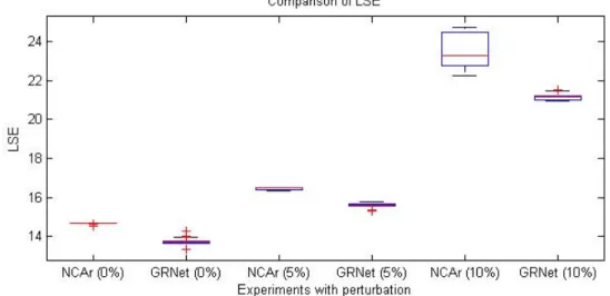
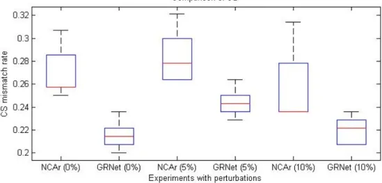
For evaluating the robustness ability of GRN, Various Gaussian perturbations (0%, 5%, and 10%) are added to the gene expression data. Our results in Figure 4.1, 4.2 reveal that GRNet is significantly superior to NCAr in both aspects of least square error and CS mismatch rate for noise-free and noisy expression data using the same dataset of Escherichia coli used by NCA [19].

(17)

Figure 4.2: Comparisons of CSdiff between GRNet and NCAr.

We run 30 silico-experiments for NCAr, GRNet, and GRNet+. In datasets: Kao_PNAS and RegulonDB_3.2, GRNet is accurate than NCAr with changing fewer regulations. As increasing LSE, [CS] array in GRNet+ comes with constraints regarding to the regulations in vivo, literature, and public database. Table 4.1: Silico and experimental results comparison

E. coli. NCAr GRNet GRNet+

LSE CS (%) LSE CS (%) LSE CS (%)

Kao_PNAS 14.66 27.02 12.91 21.95 22.04 0

RegulonDB_3.2 7.33 36.89 6.81 28.52 14.64 0

Kao_Silico 16022.7 11.4 38.09 0.22 23.42 0

Considering the first two dataset come with unknown control strength and TF activities, the Kao_Silico is simulated for known solution to validate the efficiency of GRNet. There are 10 randomly generated data in this dataset. We also take 30 runs in each dataset for both NCAr. GRNet, and GRNet+ and manipulate the average LSE, CS difference rate, and TF standard deviation (TF-SD) of [TFA]. A low standard deviation indicates that the data points tend to be very close to the mean (real [TFA] matrix). In our experiments, TF-SD in GRNet is 0.6876 compare to 44.60 in NCAr in average. In addition to GRNet, we find GRNet+ achieves no conflicts in [CS] with less LSE than GRNet. Therefore, GRNet+ can find better solutions than GRNet if the [CS] matrix is given with reliable knowledge.

(18)

Figure 4.3: Comparison of LSE between NCAr and GRNet for 10 silico-datasets

Figure 4.4: Comparison of CS conflicts between NCAr and GRNet for 10 silico-datasets

(19)

silico-datasets

4.2 Improved performance by GPU

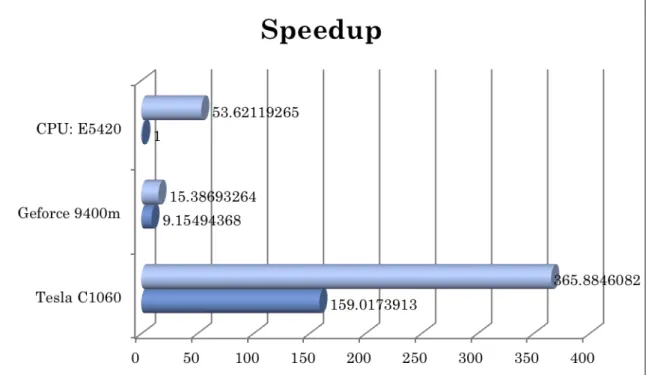
Large-scale GRNs involved with plenty of genes and TFs. In GNP, we have try two dataset for evaluating large-scale GRNs. Dataset #1 comes with 158 TFs over 2758 genes with 77 time points. Dataset #2 is similar to Dataset #1 but scale up to 30 times faster with 800 TFs over 1600 genes with 800 time points. Obviously, dataset #2 is extremely large one for simulation. In general, dataset #1 needs one week to find predicted GRNs. We manage to evaluate to time costs to manipulate matrixes multiplication in CPUs and GPUs as shown in Figure 4.6. Although the time cost to copy data from host computer and GPU device is high, we still gain about 10 times speedup for dataset #1. It means we can get GRNS with 16~17 hours for dataset #1.

Both methods in GNP: GRNet and iAEA can be parallel computed by GPU device to improve performance of reconstruction of GRNs. We plan to build GPU clusters if the requirements are increasing and budget is allowed. Currently, we only apply GPU computing of GRNs reconstruction for experimental purpose not in online services.

Figure 4.6: Speedup with CUDA architecture.

4.3 Validations of temporal GRNet

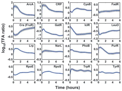
In this part, we use the Escherichia coli transition from glucose to acetate media as an example from NCA[1]. The dataset involves 16 TFs over 100 genes with 10 time points. The dynamics for 16 TFs from glucose to acetate transition is shown as Figure 4.7 from NCA.

(20)

Overall, consistent with the reduced need of building blocks during transition from glucose to acetate, activities of TFs that were involved in biosynthesis were behaving accordingly. The leu operon activator, LeuO, was inactivated during the growth arrest. The aromatic amino acid biosynthesis pathway repressors, TrpR and TyrR, were activated during this transition. TrpR binds to its ligand, tryptophan, for activation, whereas TyrR requires any of the aromatic amino acids for activation depend-ing on the target. Durdepend-ing the growth arrest, there was an apparent surplus of the aromatic amino acids, thus the two repressors involved in amino acid biosynthesis were activated to repress the biosynthetic genes. PurR is the repressor for the nucleotide biosynthesis genes using hypoxanthine or guanine as corepressors. It exhibited a sharp peak in activity initially, indicative of a reduced need for purine biosynthesis during growth arrest. The initial activation of PurR was slowly allevi-ated, suggesting that the need for nucleotide biosynthesis in-creased as growth resumed. One exception to the general reduction of biosynthesis was indicated by CysB, the activator for the synthetic genes of cysteine and uptake genes of sulfur sources. CysB is also known to be involved in glyoxylate assim-ilation and to be active under catabolite-derepressed conditions by exerting its effect on adenylate cyclase through influencing the phosphotransferase system-regulatory apparatus (15). Therefore the activation of CysB may help the cells to adapt to the new environmental condition after the carbon source tran-sition from glucose to acetate.

The global regulatory protein, Lrp, participates in coping with changes in the nutritional conditions by regulating genes in-volved in amino acid biosynthesis, transport, and degradation (16, 17). Lrp exhibits its effect on operons through various modes of action. Depending on the target operon, Lrp can be activated with or without the binding of leucine. The TFA of Lrp represents its overall impact on its membership genes. For example, as a growth lag was first observed during glucose to acetate transition, Lrp repressed genes involved in the branched

chain amino acid transport (e.g., livJ and livKHMGF) likely caused by reduced need.

Verification of TFA by cAMP Measurement.Most of the TFAs are

difficult to measure directly. However, CRP activity can be deduced from the cAMP level, which can be measured. To verify the TFA estimates of CRP, we measured the intracellular concentration of cAMP during the transition. Indeed, the time course of cAMP (Fig. 5) ratios showed the same trend of CRP activity, providing evidence in support of the NCA analysis. In particular, the peak (5 min) to valley (4 h) difference in cAMP was the same as that of CRP activity. The agreement between the time course of cAMP and the estimated TFA of CRP is a positive confirmation to the NCA methodology and the CRP connec-tivity used in the analysis.

Conclusion

DNA microarray has been successfully used as a tool in the study of differential gene expression changes in various conditions (6, 18–24). However, without the proper mathematical and

statis-Fig. 4. The dynamics of the TFA for 16 transcriptional regulators during glucose to acetate transition in E. coli. The activities for transcription regulators provide

indications of the levels of their active forms, such as phosphor-ArcA, cAMP–CRP complex, and tryptophan–TrpR complex, which may either repress or activate transcription. The solid line is the average TFA, and the shaded areas span two standard deviations (these statistics were estimated by using a bootstrap technique).

Fig. 5. The ratios of the intracellular cAMP concentration relative to the initial time point during the glucose to acetate transition. The similarity of this profile to the TFA of CRP helps to confirm the NCA approach.

Kao et al. PNAS ! January 13, 2004 ! vol. 101 ! no. 2 ! 645

MICROBIOLOGY

Figure 4.7: Time course of TF activities from NCA[1].

In purpose to comparison, partial information of regulations between TFs and genes are used in CS. TFA is defined as positive number to illustrating TF activities. However, large amounts of error in connectivity may lead to TFA profiles that are inconsistent with other existing physiological data[1]. In order to reduce the inconsistent of connectivity data and dimension, TFA is defined as positive number to prevent from inconsistent of CS in tGRNet.

(21)

Figure 4.8: TF activities deduced from tGRNet.

Compare to previous work GRNet, the several of [CS] and [TFA] are increasing as expected but the trend for control strength and TF are similar In Figure 4.8.

In addition to the previous results we obtain from tGRNet, we need some more evidence to check if our results act as real transcription factor activities. Most of TF activities are hard to measure expect CRP. The TF activities of CRP can be deduced from cAMP concentration level[37]. In Figure 4.9, CRP’s activity is similar to cAMP.

Overall, consistent with the reduced need of building blocks during transition from glucose to acetate, activities of TFs that were involved in biosynthesis were behaving accordingly. The leu operon activator, LeuO, was inactivated during the growth arrest. The aromatic amino acid biosynthesis pathway repressors, TrpR and TyrR, were activated during this transition. TrpR binds to its ligand, tryptophan, for activation, whereas TyrR requires any of the aromatic amino acids for activation depend-ing on the target. Durdepend-ing the growth arrest, there was an apparent surplus of the aromatic amino acids, thus the two repressors involved in amino acid biosynthesis were activated to repress the biosynthetic genes. PurR is the repressor for the nucleotide biosynthesis genes using hypoxanthine or guanine as corepressors. It exhibited a sharp peak in activity initially, indicative of a reduced need for purine biosynthesis during growth arrest. The initial activation of PurR was slowly allevi-ated, suggesting that the need for nucleotide biosynthesis in-creased as growth resumed. One exception to the general reduction of biosynthesis was indicated by CysB, the activator for the synthetic genes of cysteine and uptake genes of sulfur sources. CysB is also known to be involved in glyoxylate assim-ilation and to be active under catabolite-derepressed conditions by exerting its effect on adenylate cyclase through influencing the phosphotransferase system-regulatory apparatus (15). Therefore the activation of CysB may help the cells to adapt to the new environmental condition after the carbon source tran-sition from glucose to acetate.

The global regulatory protein, Lrp, participates in coping with changes in the nutritional conditions by regulating genes in-volved in amino acid biosynthesis, transport, and degradation (16, 17). Lrp exhibits its effect on operons through various modes of action. Depending on the target operon, Lrp can be activated with or without the binding of leucine. The TFA of Lrp represents its overall impact on its membership genes. For example, as a growth lag was first observed during glucose to acetate transition, Lrp repressed genes involved in the branched

chain amino acid transport (e.g., livJ and livKHMGF) likely caused by reduced need.

Verification of TFA by cAMP Measurement.Most of the TFAs are

difficult to measure directly. However, CRP activity can be deduced from the cAMP level, which can be measured. To verify the TFA estimates of CRP, we measured the intracellular concentration of cAMP during the transition. Indeed, the time course of cAMP (Fig. 5) ratios showed the same trend of CRP activity, providing evidence in support of the NCA analysis. In particular, the peak (5 min) to valley (4 h) difference in cAMP was the same as that of CRP activity. The agreement between the time course of cAMP and the estimated TFA of CRP is a positive confirmation to the NCA methodology and the CRP connec-tivity used in the analysis.

Conclusion

DNA microarray has been successfully used as a tool in the study of differential gene expression changes in various conditions (6, 18–24). However, without the proper mathematical and

statis-Fig. 4. The dynamics of the TFA for 16 transcriptional regulators during glucose to acetate transition in E. coli. The activities for transcription regulators provide

indications of the levels of their active forms, such as phosphor-ArcA, cAMP–CRP complex, and tryptophan–TrpR complex, which may either repress or activate transcription. The solid line is the average TFA, and the shaded areas span two standard deviations (these statistics were estimated by using a bootstrap technique).

Fig. 5. The ratios of the intracellular cAMP concentration relative to the initial time point during the glucose to acetate transition. The similarity of this profile to the TFA of CRP helps to confirm the NCA approach.

Kao et al. PNAS ! January 13, 2004 ! vol. 101 ! no. 2 ! 645

MICROBIOLOGY

Figure 4.9: Comparisons of cAMP concentration during glucose to acetate transition are made between experiment and tGRNet. Left side is observed from biological experiment[37]. Right size is the TF activities

from tGRNet.

4.4 User guidance to use GNP

GNP is used for user to analysis GRNs with interested genes. Therefore, we simplified the complexity of operations and provide a flowchart to guide user how to start. Figure 4.10 is the flowchart of GNP. First of all, user must have microarray data for their research topics. They can choose only interested genes for analysis. GNP currently support .csv file only. The first raw is the definitions of time points and followed by expression profiles for each genes. The expression level can be log ratio number and separated by ‘\t’. Then, you can submit to GNP to retrieve connectivity data from our database or specify regulations by your own domain knowledge. The most important step is choosing the regulations you interested that is not published yet. With GNP, we can predict the regulations of unknown and show the control strength for each regulation.

After all, all you need to do is waiting for email to access your results. You may need to wait hours or days, even weeks depends on the scale of GRNs. Finally, the results contains a network topology as Figure 4.11 and two detailed [CS] and [TFA].

(22)

Expression profiles for interested

genes

Submit to GNP Start to analysis

Retrieve connectivity data Determine unknown regulations Predicted GRNs With weighted control strength Finished

Find new regulations Database built by sub-‐project Validate the unknown regulations by experiments Finish

Figure 4.10: Flowchart to use GNP for reconstructing GRNs. Orange rectangles are actions user need to handle.

Figure 4.11: E. coli (from Kao’s data) GRNs predicted by GNP.

4.5 Case study with experimental validations

When obtaining gene regulatory networks with the regulatory control strategy, the biological experiments for validation should be conducted. To validate the regulations between genes we found, one step inactivation of chromosomal genes is performed to knock out investigated gene once per time. We use RT-PCR to measure amounts of mRNA expression in small scale with heavy and complicated routines for

(23)

large scale GN in our experimental validation. Through these real experiments, the obtained computational model and regulatory control strategy can be verified. For some complex biological mechanism researches, this approach can help them to clarify the interesting topics.

Our Co-PIs, Prof. Tseng’s Lab provide us microarray data of E. coli during transition from anaerobic to aerobic conditions for analysis. The expression profiles are shown in Figure 4.12. In this part, we aim to figure out what GNP is capable with our iAEA and GRNet. Hence, we discuss the unknown regulations GNP predicted of CRP and Fnr over fumC.

Figure 4.12: The experssion profiles for both involved genes and TFs.

!

Figure 4.13: Connectivity data of E. coli data is shown. There are 6 regulations are mark as unknown with symbol x.

In Table 4.2 and 4.3, we compare the known regulations between GRNet, iAEA, Tseng’s Lab, and RegulonDB. We found our predictions for CRP over fumC and Fnr are matched. In case of the dimensions of the known variables are lower than the unknown (in this example we have 3x4 unknown in [E] v.s. 3x3 partial known in [CS] and 3x4 unknown in [TFA]), the solutions are not fixed very well. But GRNet provides stable solutions for biologists to analysis before they start to perform microarray experiments. GNP intends to find sufficient solutions to support us to reconstruct GRNs.

(24)

Table 4.2: Comparison between GRNet, RegulonDB, and Tseng’s Lab in 30 runs

Tseng’s Lab RegulonDB 7.2 GRNet

ArcA CRP Fnr ArcA CRP Fnr ArcA CRP Fnr

fumA -‐ + -‐ -‐ + -‐ -‐ + -‐

fumB + x + + + + + + +

fumC -‐ + -‐ -‐ x x -‐ + -‐

Table 4.3: Comparison between iAEA, RegulonDB, and Tseng’s Lab in 50 runs

Tseng’s Lab RegulonDB 7.2 iAEA

ArcA CRP Fnr ArcA CRP Fnr ArcA CRP Fnr

fumA -‐ + -‐ -‐ + -‐ -‐ + -‐ fumB + ? + + + + + -‐ + fumC -‐ + -‐ -‐ x x -‐ + -‐ arcA ? + ? x x +-‐ x + +-‐ crp ? + ? x +-‐ x +-‐ + -‐ fnr -‐ ? -‐ -‐ x -‐ -‐ +-‐ -‐

In Table 4.4, we have different combinations in regulation of CRP and Fnr over fumC, ‘X’, ‘-‘,’+’, ‘?’ present no regulation, repressor, activator, and unknown regulations respectively. GRNet can satisfy the expression profiles sufficiently no matter of the hypothesis we have in the beginning.

Table 4.4: Combination of regulations for Fnr and CRP over fumC.

Fnr\CRP X -‐ + ?

X 2.95E-‐12 1.27E-‐12 4.20E-‐13 7.29E-‐13

-‐ 1.21E-‐12 1.32E-‐12 1.38E-‐12 1.54E-‐12

+ 5.59E-‐12 1.02E-‐12 2.59E-‐12 1.11E-‐12

? 4.40E-‐12 3.99E-‐12 2.70E-‐12 1.41E-‐12

Figure 4.14: Expression profiles with different priori knowledge in [CS].

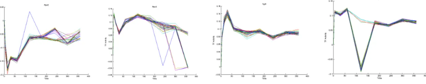
In different combitions of Fnr and CRP over fumC, comparions are shown in Figure 4.14. There are four data in this figure, the purple and blue line represent real and predicted expression profile respectively. We run 30 runs of GRNet and get the average of [CS] and [TFA] to obtaion predicted expression profile. As shown in the figure, the expression profiles are fitted well even the various are in [CS] and [TFA]. Also, the

(25)

red and green lines present mutation of CRP and Fnr over fumC. We think the red line make sense to the mutation of CRP over fumB and fumC but not to fumA after discussion with Tseng’s Lab. The concentrations of specific genes are similar to real expression profiles of fumA, fumB, and fumC as show in Figure 4.14. With helps of GNP, we found the new regulations of CRP and Fnr over fumC and verified in biological experiments.

Figure 4.15: Expression profiles with different priori knowledge in [CS] with knock-out of CRP and Fnr.

5. Conclusions and future works

As a convenient and efficient platform of reconstructing gene regulatory network is available, biologists can obtain accurate computational models of gene networks to simulate the dynamics of interested gene expressions. With the help of simulated dynamics, the desired regulatory control mechanism can be designed for drug design and other purposes. However, the complex regulatory relationships between genes make the optimal regulatory control difficult to realize manually. Discussions of predicted GRNs are interested for biologists to define the range of control strength or transcription factors activities between regulations.

5.1 Refining the platform incrementally

A use-friendly, reliable, and fast-response multi-user platform would be evaluated and tested from many users using various kinds of applications. The provided functions of the platform would be increased gradually after rigorous tests. To maintain the platform work continuously, it is desirable to carefully design and test the system. Therefore, sufficient resources such as human resource and computer servers are necessary. Some tasks are listed as follows:

l Collect experimental data from web lab for specific species for testing and refining the system. l Collect the achievement of using the platform for increasing the experience of inferring GRNs. l Prepare the documents and help service for using the platform.

l Maintain and manage the gene network platform.

5.2 Experimental validations

When obtaining gene regulatory networks with the regulatory control strategy, the biological experiments for validation should be conducted. To validate the regulations between genes we found, one step inactivation of chromosomal genes is performed to knock out investigated gene once per time. We use RT-PCR to measure amounts of mRNA expression in small scale with heavy and complicated routines for large scale GRNs in our experimental validation. Through these real experiments, the obtained computational model and regulatory control strategy can be verified. For some complex biological mechanism researches, this approach can help them to clarify the interesting topics.

(26)

6. Related research achievements

6.1 Journal papers

Journal papers are from 2008 (* corresponding author) as follows:

1. H.-L. Huang, F.-L. Chang, S.-J. Ho, L.-S. Shu, W.-L. Huang, and S.-Y. Ho*, “FRKAS: Knowledge

Acquisition Using a Fuzzy Rule Base Approach to Insight of DNA-Binding Domains/Proteins,” accepted by Protein and Peptide Letters, 2011. (SCI)

2. S.-Y. Ho, C.-Y. Chao, H.-L. Huang, T.-W. Chiu, P. Charoenkwan, and E. Hwang*, “NeurphologyJ: an automatic neuronal morphology quantification method and its application in pharmacological discovery,” BMC Bioinformatics, 12:230, 2011. (SCI)

3. H.-L. Huang, I-C. Lin, Y.-F. Liou, C.-T. Tsai, K-T. Hsu, W,-L. Huang, S.-J. Ho, and S.-Y. Ho*, “Predicting and analyzing DNA-binding domains using a systematic approach to identifying a set of informative physicochemical and biochemical properties”, BMC Bioinformatics, 12(Suppl 1):S47, 2011. (SCI)

4. Hsin-Nan Lin, Ting-Yi Sung, S.-Y. Ho and Wen-Lian Hsu, “Improving protein secondary structure prediction based on short subsequences with local structure similarity,” BMC Genomics, 11(Suppl 4):S4, 2010 (SCI)

5. C.-H. Hung, H.-L. Huang, K.-T. Hsu, S.-J. Ho and S.-Y. Ho, ”Prediction of non-classical secreted proteins using informative physicochemical properties." Interdiscip Sci Comput Life Sci 2: 263-270, 2010.

6. Hsin-Nan Lin, Ching-Tai Chen, Ting-Yi Sung, S.-Y. Ho, and Wen-Lian Hsu* "Protein subcellular localization prediction of eukaryotes using a knowledge-based approach," BMC Bioinformatics, 10(Suppl 15):S8, 2009. (SCI)

7. W.-L Huang, C.-W Tung , H.-L Huang and S.-Y. Ho*, "Predicting protein subnuclear localization using GO-amino-acid composition features," BIOSYSTEMS, Vol 98 (2), pp. 73-79, 2009. (SCI)

8. H.-Y Huang, H.-Y Chang, C.-H Chou, C.-P Tseng, S.-Y. Ho, C.-D Yang, Y.-W Ju and H.-D Huang*, "sRNAMap: genomic maps for small non-coding RNAs, their regulators and their targetsin microbial genomes," Nucleic Acids Research, vol. 37, Database issue, 2009. (SCI)

9. C.-T. Tsai, W.-L. Huang, S.-J. Ho, L.-S. Shu and S.-Y. Ho*, "Virulent-GO: Prediction of virulent proteins in bacterial pathogens utilizing Gene Ontology terms," International Journal of Biological and Life Sciences, vol. 5, no. 4 pp. 159-166, 2009. (SCI)

10. C.-W. Tung and S.-Y. Ho*, "Computational identification of ubiquitylation sites from protein sequences,” BMC Bioinformatics, 9:310, 2008. (SCI)

11. W.-L. Huang, C.-W. Tung, S.-W. Ho, S.-F. Hwang and S.-Y. Ho*, ”ProLoc-GO: Utilizing informative Gene Ontology terms for sequence-based prediction of protein subcellular localization,” BMC

Bioinformatics, 9:80, 2008. (SCI)

(27)

simulated annealing algorithm for designing robust PID controllers,” IEEE Trans. Systems, Man, and Cybernetics Part A ─Systems and Humans 38 (2), pp. 319-330, 2008. (SCI, EI)

13. S.-Y. Ho, H.-S. Lin, W.-H. Liauh and S.-J. Ho*, "OPSO: Orthogonal Particle Swarm Optimization and Its Application to Task Assignment Problems," IEEE Trans. Systems, Man, and Cybernetics Part A ─Systems and Humans 38 (2), pp. 288-298, 2008. (SCI, EI)

6.2 Submitted and under revision papers

14. W.-L. Huang, C.-W. Tung, C. Liaw and S.-Y. Ho*, “Predicting subcellular localization of eukaryotic and prokaryotic proteins using increasingly informative Gene Ontology terms,” PLoS ONE, 2011. (under revision) (SCI)

15. C.-W. Tung, M. Ziehm, A. Kämper, O. Kohlbacher*and S.-Y. Ho*, “POPISK: T-cell reactivity

prediction using support vector machines and string kernels,” BMC Bioinformatics, 2011 (under revision). (SCI)

16. W.-L. Huang, C.-W. Tung and S.-Y. Ho*, “Predicting promoters by designing an informative feature set of DNA sequence descriptors and using an inheritable bi-objective genetic algorithm,” Submitted to Information Science, 2011. (SCI)

6.3 International Conference papers

Conference papers are from 2009 as follows:

1. H.-L. Huang., T.-F. Kao., P. Charoenkwan., W.-L. Huang, S.-J. Ho and S.-Y. Ho*, 2012, “Estimating

solubility scores of dipeptides and residues for predicting proteins solubility,” The Tenth Asia Pacific Bioinformatics Conference, Melbourne, Australia, 17-19 January 2012.

2. C.-T. Tsai, W.-L. Huang, C. Liaw, C.-W. Tung, H.-L. Huangand S.-Y. Ho*, 2012, “Virulence-iGO:

Predicting virulence factors in pathogenic bacteria using informative Gene Ontology terms,” The Tenth Asia Pacific Bioinformatics Conference, Melbourne, Australia, 17-19 January 2012.

3. H.-C. Lee, S.-J. Ho, L.-S. Shu, F.-L. Chang, S.-Y. Ho and H.-L. Huang*, 2012, “Optimization method of predicting enzyme mutant activity from sequences by identifying a set of informative physicochemical properties,” The Tenth Asia Pacific Bioinformatics Conference, Melbourne, Australia, 17-19 January 2012.

4. H.-L. Huang, Y.-H. Lin, W.-L. Huang and S.-Y. Ho*, 2011, “Intelligent triple-objective genetic

algorithm for selecting informative Tag SNPs,” The 22nd_{International Conference on Genome}

Informatics, Korea, Dec. 5-7, 2011.

5. H.-L. Huang, S.-B. C., Y.-H. Chen, and S.-Y. Ho*, 2011, “Optimization approach to estimation of

kinetic parameters for modelling metabolic pathways of muscle glycogenolysis,” The 22nd International

Conference on Genome Informatics, Korea, Dec. 5-7, 2011.

6. L.-S. Shu, H.-L. Huang, S.-J. Ho, and S.-Y. Ho*, 2011, “Establishing large-scale gene regulatory networks using a gene-knowledge-embedded evolutionary computation method,” IEEE International Conference on Computer Science and Automation Engineering, June 10-12, 2011, Shanghai, China. 7. H.-L. Huang, F.-L. Chang, S.-J. Ho, L.-S. Shu, and S.-Y. Ho*, 2011, “Interpretable knowledge

(28)

International Conference on Computer Science and Automation Engineering, June 10-12, 2011, Shanghai, China.

8. H.-L. Huang, I-C. Lin, Y.-F. Liou, C.-T. Tsai, K.-T. Hsu, W.-L. Huang, S.-J. Ho, and S.-Y. Ho*, 2011, “Predicting and analyzing DNA-binding domains using a systematic approach to identifying a set of informative physicochemical and biochemical properties, APBC 2011, Korea, Jan. 11-14.

9. C. Liaw, C.-W. Tung, S.-J. Ho and S.-Y. Ho*, 2010, “Sequence-based Prediction Of Gamma-turn Types Using A Physicochemical Property-based Decision Tree Method”, International Conference on Computational Biology, WASET 2010 Tokyo, May 26-28, 2010, Japan.

10. C.-W. Tung, C. Liaw, S.-J. Ho and S.-Y. Ho*, 2010, “Prediction of protein subchloroplast locations using Random Forests”, International Conference on Computational Biology, WASET 2010 Tokyo, May 26-28, 2010, Japan.

11. Y.-J. Lin, H.-L. Huang, K.-T. Hsu, and S.-Y. Ho*, 2010, “Designing predictors of DNA-binding proteins using an efficient physicochemical property mining method,” The 2nd International Conference on Computer and Automation Engineering (ICCAE2010), Singapore, Feb. 26-28.

12. W-L Huang, C-W Tung, S-Y Ho*, 2010, ”Human Pol II promoter prediction by using nucleotide property composition features.” The International Symposium on Biocomputing (ISB) Feb 15-16, Calicut, Kerala, India.

13. C.-H. Hung, H.-L. Huang, K.-T. Hsu, S.-J. Ho and S.-Y. Ho*, 2009, ”Prediction of non-classical secreted proteins using informative physicochemical properties." The International Conference on Computational and Systems Biology (ICBB) October 9-11, Shanghai, China.

14. K.-T. Hsu, H.-L. Huang, C.-W. Tung, Y.-H. Chen, and S.-Y. Ho*, 2009, "Analysis of physicochemical properties on prediction of R5, X4 and R5X4 HIV-1 coreceptor usage," International Conference on Bioinformatics and Bioengineering (ICBB), May 27-29, Tokyo, Japan.

15. C.-T. Tsai, W.-L. Huang, S.-J. Ho, L.-S. Shu, and S.-Y. Ho*, 2009, "Virulent-GO: Prediction of virulent proteins inbacterial pathogens utilizing Gene Ontology terms," International Conference on Bioinformatics and Bioengineering (ICBB), May 27-29, Tokyo, Japan.