Tourism multipliers and capacity utilization- A case study of Taiwan tourism
hotel
Ya-Yen Sun
Assistant Professor
Department of Kinesiology, Health, and Leisure Studies (DKHL) National University of Kaohsiung
No. 700, Kaohsiung University Rd., Nan Tzu Dist., 811 Kaohsiung, Taiwan
Tel: 886-7-5919217 Fax: 886-7-5919264 E-mail: [email protected]
Tourism multipliers and capacity utilization- A case study of Taiwan
tourism hotels
ABSTRACT
Input-Output (I-O) model, a popular tourism economic impact evaluation method, assumed the stability of economic ratios and regional multipliers during the evaluation period. Constant technical coefficients and fixed economic ratios of employee compensation, jobs, and profitability are applied when calculating total impacts. For manufacturing sectors, constant multipliers within a short term period may resent a reasonable picture of the real-world production function. Tourism, however, is composed of a variety of services, which total output and factor inputs are strongly influenced by capacity utilization. A conceptual model is proposed in this paper to indicate that a shift in capacity utilization for perishable services will lead to economies of scale in inputs, price changes in final output, and possible substitution between input factors, especially between capital and labor. These factors simultaneously influence the stability of I-O ratios and tourism multipliers. Using constant economic ratios and multipliers in the tourism economic impact analysis, as traditional I-O analysis has assumed, will therefore lead to biases, especially on the value added component.
Introduction
Input-Output (I-O) analysis has been extensively adopted to estimate tourism economic impacts in the tourism planning and management procedures from both national and regional perspectives. Advantages of I-O analysis are 1) its flexibility to evaluate economic impacts from the general equilibrium perspective based on different temporal and spatial scales, 2) its ability to monitor the economic impacts of individual groups who have distinct spending patterns, and 3) the ease of interpretation and convenience of data
availability (Blake, 2000; Briassoulis, 1991; Fletcher, 1989).
Input-Output analysis computes tourism economic impacts by first converting the final demand changes (visitor spending, investment) into direct effects in terms of jobs, personal income, tax and value added using economic ratios pertained to the regional economy. Secondary effects are then computed by multiplying the direct effects with the regional multipliers, which are resulted from the inter-industry dependences. Total impacts of employment, for example, are determined by three factors: jobs to sales ratios, regional sales multipliers, and final demand changes. The first factor, the jobs to sales ratio, represents the average ratio of labor inputs to production, regional sales multipliers indicate the structure of the local economy, and final demand changes specify the total amount of money injected.
Three principal assumptions employed in an I-O analysis are 1) the output of each sector is produced with a unique set of inputs, 2) the amount of inputs required is solely determined by the level of output, and 3) there are no capacity constraints on the production process (Miller & Blair, 1985; Otto & Johnson, 1993). Based on these assumptions,
economic impact is solely determined by final demand changes. In other words, I-O models have assumed the stability of economic ratios and regional multipliers during the evaluation period (typically 2 to 5 years). Constant technical coefficients and fixed economic ratios of labor cost, employment, and profitability are applied when calculating total impacts
regardless of the level of demand changes as well as the level of sector capacity. A sector operating at the 40% capacity is assumed to have the same cost structures as one at the 80% capacity.
For manufacturing sectors, constant economic ratios, such as jobs to sales ratio, and regional multipliers within a short term period may provide a satisfactory portray of the real-world production function and offer estimates with acceptable errors (G. R. West, 1995). The tourism industry, however, is perceived as a combination of sectors and most of them offer services that are time perishable, such as lodging, entertainment, and transportation. These time-perishable services have distinct characteristics such as simultaneity and perishability in their production and consumption process. Specifically, capacity utilization (CU), the ratio of actual used (consumed) products to the total available products, is a distinct measurement for time-perishable services for explaining changes in the rate of investment, labor productivity and inflation (Berndt and Morrison, 1981).
The purposes of this paper are first to provide a conceptual framework that examines the stability of I-O ratios and tourism multipliers from the perspective of capacity utilization. A case study of Taiwan tourist hotel is adopted to present the relationship between two I-O ratios (jobs to sales ratio and income to sales ratio) and capacity utilization (occupancy rates).
Conceptual framework
One primary limitation of the I-O analysis is that constant technical coefficients and fixed economic ratios of labor cost, employment, and profitability are applied when
calculating total impacts. For manufacturing sectors, constant regional multipliers within a short term period may resent a reasonable picture of the real-world production function (G. R. West, 1995). Tourism, however, is not a single acknowledged sector (Fletcher, 1989; Smith, 1994). It covers a combination of industries, most providing time perishable services, such as
lodging, entertainment, and transportation. These services have distinct production and consumption process from manufactured goods.
The major characteristics of services are intangibility, simultaneity and perishability. Intangibility indicates that services are not solid products and cannot be stored for repeated use (perishability). Simultaneity implies that the production and the consumption of services occur at the same point in time and location. Unlike manufactured goods, the unused
perishable products (e.g., hotel rooms or airline tickets) cannot be resold somewhere else and the associated sales are lost forever. Second, high fixed costs are incurred in the production process regardless of the demand level (Kimes, 1989; Lewis & Chambers, 1989). The marginal cost of an additional unit is relatively low unless at full capacity. The operational objective, therefore, is to maximize profits instead of minimizing costs (Berman, 1994).
One approach to generate maximum profits for perishable products is through price discrimination in which the price is determined based on the level of demand and unused capacity. Accommodations and air transportation generally employ this pricing strategy (referred as yield management by the academicians). Due to high fixed capacity and product perishability, the profit level of many service firms is greatly tied to capacity utilization (Allen, 1988).
The third general characteristic of service industries is that they are labor and capital intensive (Mullins, 1993). Because of limited productivity gains through technological progress, accommodations and restaurants tend to make the best use of existing labor to accommodate additional demands (Hollenstein, 2001; Peneder, Kaniovski, & Dachs, 2003; Smeral, 2003).
Due to these fundamental characteristics - perishability, intangibility and simultaneity, cost structures of perishable services are determined by the number of units consumed (sold), instead of the number of units produced. This has led to a distinct measurement for
time-perishable services: capacity utilization (CU), the ratio of actual used products to some measure of potential outputs (Nelson, 1989; Ng, Wirtz, & Lee, 1999). Based on Berndt and Morrison (1981), CU is an important factor in explaining changes in the rate of investment, labor productivity and inflation for services.
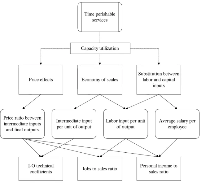
A conceptual model connecting capacity utilization and the I-O framework is presented in Figure 1. It hypothesizes that a shift in utilization for perishable services will lead to economies of scale in both labor and material inputs (Miller & Blair, 1985), price changes in final output (Arenberg, 1991), and possible substitution between input factors, especially between capital and labor (Krakover, 2000; G. West & Gamage, 2001). The pricing strategy will modify the price ratio of intermediate inputs to final output1; the
economies of scale change the input ratio of labor and materials; and the substitution pattern between labor and capital adjusts the average salary per employee. These factors
simultaneously affect the I-O technical coefficients, jobs to sales ratios, and personal income to sales ratio.
1
Price change may result in technical substitution between different intermediate inputs. However, it has been argued that a major swing in relative price is required before substitution takes place (Rose & Miernyk, 1989).
Time perishable services
Average salary per employee Labor input per unit
of output Price ratio between
intermediate inputs and final outputs
Capacity utilization
Economy of scales Substitution between labor and capital inputs Price effects
Intermediate input per unit of output
Price effects Economy of scales
Substitution between labor and capital
inputs
I-O technical
coefficients Jobs to sales ratio
Personal income to sales ratio
Figure 1. The Conceptual Framework of Capacity Utilization and I-O Analysis
As demonstrated in Equation 1, economies of scale in input materials and price changes of the final product would modify the I-O technical coefficients. Economies of scale in labor inputs (labor efficiency) and changes in the price of the final product would adjust the jobs to sales ratios (Equation 2). Personal income to sales ratios on the other hand are influenced concurrently by labor inputs, output price and average salary per employee (Equation 3).
α ij = qij *
j i
P P
= f (economy of scale in materials, price ratio of inputs to final product)
(Equation 1) Where αij = technical input coefficient = output of industry i that is bought by industry j
to produce one unit of product j
qij = physical input coefficient = physical output of industry i required to produce a
physical unit output of industry j Pi = price of product i
Pj = price of product j
Jobs to sales ratio =
sales Total employees Total = sold units Total employees Total * product final the of Price 1
= f (labor productivity, price of the final product) (Equation 2)
Personal income to sales ratio =
sales Total wages Total = sold units Total employees Total * product final the of Price 1
* Average salary per employee
= f (labor productivity, price of the final product, average salary per employee) (Equation 3)
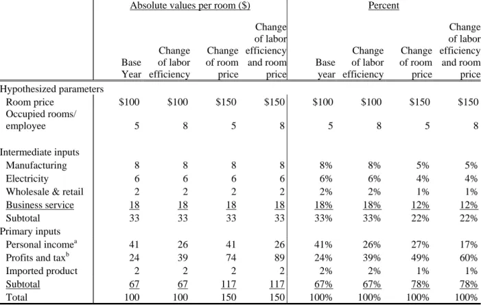
A hypothesized example is used in Table 1 to demonstrate changes in the cost structure by allowing output price and labor ratio to vary. Labor ratio, in this example, is defined as number of final products sold per employee, which can be regarded as a measure of labor efficiency. The base year cost function of the accommodation sector is presented first
using the I-O coefficients from the 1999 Taiwan Input-Output table. Assuming a room price of $100, thirty-three percent of the cost will go to intermediate inputs, such as business services and manufacturing, 41% will be allocated to employee compensation, 2% to
imported products, and 24% to profits and taxes. In this instance, the labor efficiency equates to the number of occupied rooms per worker. In the base year (the year I-O table is
compiled), one worker is hypothesized to support five occupied rooms at an occupancy rate of 50%.
By allowing labor efficiency and output price to change along with occupancy rates, the cost function and profitability, in absolute value and relative percent, are different. For example, if labor efficiency is improved from serving 5 occupied rooms per employee to 8 occupied rooms per employee, the relative ratio of labor cost is reduced per room while the ratio of input materials remain unchanged. In this instance, type I sales multipliers will
remain unchanged from the base-year level but the jobs to sales ratio will decrease, indicating that fewer jobs are supported with the same amount of hotel sales. A change in room price, however, will affect the relative cost ratio for both intermediate inputs and labor inputs. In this case, the elasticity of changes in I-O multipliers will be determined simultaneously by three factors: labor efficiency, the price of input materials, and the price of final products. For example, if the average room price rises from $100 to $150, assuming the input materials still cost $33 per room and one employee supports 5 occupied rooms (unchanged from the base-year level), the absolute monetary costs of intermediate inputs and labor are unaffected but the relative ratio of costs is reduced. This will then lead to reduced type I sales multipliers and jobs multipliers.
Table 1. An Example of the Cost Structure for a Hotel Room by Absolute Value and Percent
Absolute values per room ($) Percent
Base Year Change of labor efficiency Change of room price Change of labor efficiency and room price Base year Change of labor efficiency Change of room price Change of labor efficiency and room price Hypothesized parameters Room price $100 $100 $150 $150 $100 $100 $150 $150 Occupied rooms/ employee 5 8 5 8 5 8 5 8 Intermediate inputs Manufacturing 8 8 8 8 8% 8% 5% 5% Electricity 6 6 6 6 6% 6% 4% 4%
Wholesale & retail 2 2 2 2 2% 2% 1% 1%
Business service 18 18 18 18 18% 18% 12% 12%
Subtotal 33 33 33 33 33% 33% 22% 22%
Primary inputs
Personal incomea 41 26 41 26 41% 26% 27% 17%
Profits and taxb 24 39 74 89 24% 39% 49% 60%
Imported product 2 2 2 2 2% 2% 1% 1%
Subtotal 67 67 117 117 67% 67% 78% 78%
Total 100 100 150 150 100% 100% 100% 100%
a
Assuming the average salary per employee is fixed. When an employee can clean more room, for example, the average wage cost per room is reduced (marginal labor cost per room is decreasing).
b
Profits and tax are computed by deducting the rooms sales with costs on intermediate inputs, imported products and labor.
Based on this example, an increased room price and more efficient labor usage result in a reduced input costs and subsequently, higher operating surplus. Allowing the average salary per employee to vary creates a more complicated example. Any change in the input factors will lead to modifications of the cost structure. The assumption of Constant Returns to Scale (CRTS), which indicates fixed input costs, labor expenses, and profitability in relation to sales volume, is not valid when output price, labor efficiency, and average wages are allowed to vary.
Case-study: Tourist hotels in Taiwan
Based on the proposed model in Figure 1, shifts in capacity utilization will lead to modifications of technical input coefficients and economic ratios for the value added
components. In this study, the primary focus is to relax the assumption of constant value added components (the dynamics of job and income) through modification of jobs to sales ratio and income to sales ratio in the I-O model while the technical input coefficients remain constant. Empirical data of tourist hotel operation was adopted to study the stability of two economic ratios (jobs to sales ratio and income to sales ratio) with respect to capacity utilization. Econometric models were constructed to determine the relationship of (1) occupancy rates and jobs per NT$ million hotel sales, and (2) occupancy rates and personal income per NT$ million hotel sales using two panel data (1999-2003). Geographic location, consumer price index, and hotel scales were included as control variables in the regression equation to account for differences between hotels (Liu & Var, 1982; Pan). Regression analysis was performed within the Statistical Package for Social Science (SPSS) and Stata using the stepwise approach. The function form was determined by comparing adjusted R-square values across 11 function forms (curve-estimation process in the SPSS program). Multicollinearity and autocorrelation were examined during the analysis. Corrections were performed when needed.
Results
Job to Sales Ratio
A log linear functional form best captures the relationship between hotel jobs to sales ratios and occupancy rates (Equation 4). This function form has higher adjusted R-square value than others. No multicollinearity is detected among the independent variables, and no heteroskedasticity is detected among the error terms.
ln (jobs to sales ratio) = α + β1* occupancy rate + β2* hotel scale + β3* consumer price
index + β4* central Taiwan + β5* southern Taiwan + β6* eastern Taiwan + error term (0,
) (Equation 4)
2
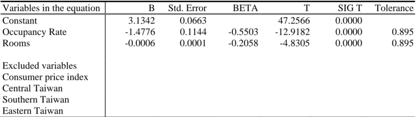
Occupancy rates and hotel scales (number of rooms) are significant in determining jobs to sales ratios at the 95% confidence level. The consumer price index and three dummy variables (representing three regions in Taiwan) are not significant (Table 2). Jobs to sales ratios are negatively correlated with occupancy rates. A rise in occupancy rate leads to fewer jobs per million sales (Equation 5). Due to the non-linear functional form, the percentage changes in jobs to sales ratio are not constant at different occupancy levels. A 5% increase from 80% to 85% in occupancy, for example, will lead to a smaller reduction in jobs to sales ratios than a 5% increase from 40% to 45%.
Table 2. Regression Statistics for the Log Jobs to Sales Ratio
Variables in the equation B Std. Error BETA T SIG T Tolerance
Constant 3.1342 0.0663 47.2566 0.0000
Occupancy Rate -1.4776 0.1144 -0.5503 -12.9182 0.0000 0.895
Rooms -0.0006 0.0001 -0.2058 -4.8305 0.0000 0.895
Excluded variables Consumer price index Central Taiwan Southern Taiwan Eastern Taiwan
Stepwise analysis is employed with 0.05 to enter and 0.10 to remove. Adjusted R-Squared = .415 ; F-Value = 128.820 (p value = 0.0000); Number of cases = 361
ln (jobs to sales ratio) = 3.1342 –1.4776*occupancy rate - 0.0006* rooms
(Equation 5)
Personal Income to Sales Ratio
Personal income to sales ratios are modeled as a linear function of occupancy rates, the number of rooms per establishment, consumer price index, and regional dummy
variables. The linear function form is applied because of its high adjusted R-square values than other forms (Equation 6).
Personal income to sales ratio = α + β1* occupancy rate + β2* hotel scale + β3* consumer
price index + β4* central Taiwan + β5* southern Taiwan + β6* eastern Taiwan + error
No multicollinearity is observed in the independent variables but some level of heteroskedasticity is discovered among the error terms. Variances of the coefficients are re-calculated using the Huber-White sandwich estimation, which corrects the bias of
heteroscedasticity. The correction provides larger variances (robust standard error) for the constant and occupancy rates in the equation, but the recomputed standard error does not change the significance of the independent variables.
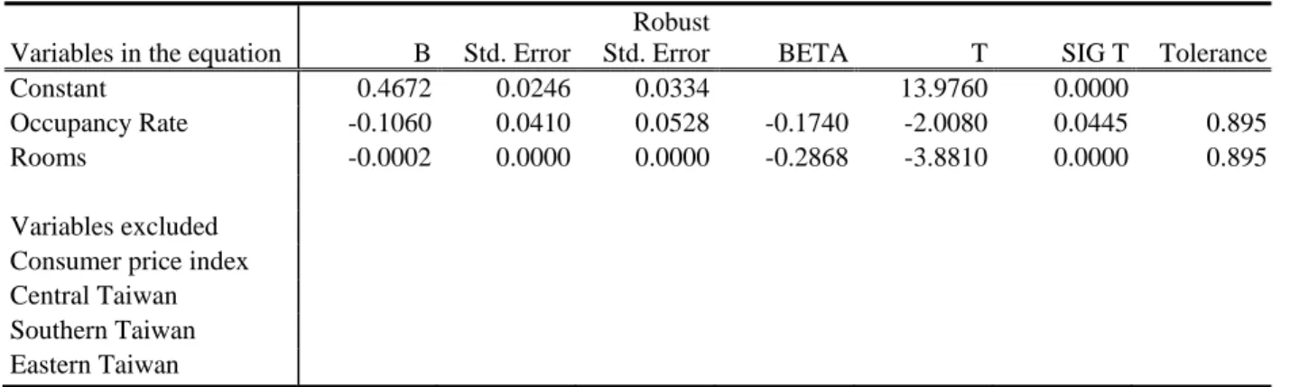
Occupancy rates and hotel scales (number of rooms) are significant in determining personal income to sales ratios at the 95% confidence level (Table 3). Income to sales ratios and occupancy rates are negatively correlated, indicating that a rise in the occupancy rate leads to a smaller percentage of sales going to employee compensation. A one percent increase in occupancy rate would yield a decrease of 0.11 in the income to sales ratio, ceteris paribus (Equation 7).
Table 3. Regression Statistics for the Income to Sales Ratio Variables in the equation B Std. Error
Robust
Std. Error BETA T SIG T Tolerance
Constant 0.4672 0.0246 0.0334 13.9760 0.0000
Occupancy Rate -0.1060 0.0410 0.0528 -0.1740 -2.0080 0.0445 0.895
Rooms -0.0002 0.0000 0.0000 -0.2868 -3.8810 0.0000 0.895
Variables excluded Consumer price index Central Taiwan Southern Taiwan Eastern Taiwan
Stepwise analysis is employed with 0.05 to enter and 0.10 to remove. Adjusted R-Squared = .1368; F-Value = 18.0350 (p value = 0.0000); Number of cases = 216
Income to sales ratio = 0.4672 - 0.1060*occupancy rate - 0.0002 *rooms (Equation 7)
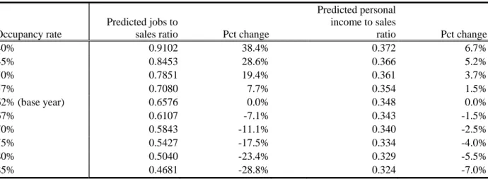
The predicted job and income to sales ratios are estimated using Equation 6 and 7 under different occupancy rates. With the average occupancy rate of 62% in 1999 and an average 253 rooms per hotel, a five percent increase in occupancy rates would lead to a 7%
decrease in job ratios, and a 1.5% reduction in income ratios (Table 4). A five percent decrease in occupancy rates, on the other hand, would raise the job ratio by 8% and increase the income ratio by 1.5%.
Table 4. Predicted Jobs and Income Ratios for Taiwan Tourist Hotels
Occupancy rate
Predicted jobs to
sales ratio Pct change
Predicted personal income to sales ratio Pct change 40% 0.9102 38.4% 0.372 6.7% 45% 0.8453 28.6% 0.366 5.2% 50% 0.7851 19.4% 0.361 3.7% 57% 0.7080 7.7% 0.354 1.5% 62% (base year) 0.6576 0.0% 0.348 0.0% 67% 0.6107 -7.1% 0.343 -1.5% 70% 0.5843 -11.1% 0.340 -2.5% 75% 0.5427 -17.5% 0.334 -4.0% 80% 0.5040 -23.4% 0.329 -5.5% 85% 0.4681 -28.8% 0.324 -7.0% Conclusion
Empirically, jobs to sales ratios and personal income to sales ratios for the hotel sector were not constant with respect to occupancy rates and hotel scale. Using constant economic ratios in the tourism economic impact analysis, as traditional I-O analysis has assumed, will therefore lead to biases, especially on the value added component. The direction and
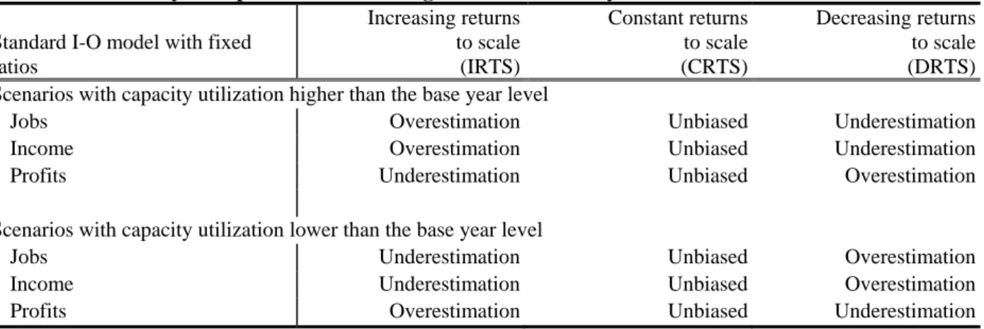
magnitude of biases associated with traditional I-O ratios can be approached from the perspective of returns to scale and cost structures. The coefficients in the standard I-O table represent the average production function, indicating the general performance of businesses at a specific level of supply and demand in a year. For services with constant returns to scale, the standard I-O model provides unbiased impact estimates regardless of the level of capacity utilization (Table 5). For services with increasing returns to scale (IRTS), the standard I-O model overestimates jobs and total income, and underestimates profits when applying average coefficients to scenarios with capacity utilization higher than the base-year point.
The biases result from greater labor efficiency, economies of scale, and substitutions between capital and labor inputs under higher demand. For services following decreasing returns to scale, the biases will be in the opposite direction.
Table 5. Sensitivity of Impact Estimation using Fixed I-O Ratios by Returns to Scale Standard I-O model with fixed
ratios Increasing returns to scale (IRTS) Constant returns to scale (CRTS) Decreasing returns to scale (DRTS) Scenarios with capacity utilization higher than the base year level
Jobs Overestimation Unbiased Underestimation
Income Overestimation Unbiased Underestimation
Profits Underestimation Unbiased Overestimation
Scenarios with capacity utilization lower than the base year level
Jobs Underestimation Unbiased Overestimation
Income Underestimation Unbiased Overestimation
Profits Overestimation Unbiased Underestimation
The proposed changing tourism multipliers apply whenever the policy being
evaluated causes changes in capacity utilization from the base year point (the year I-O table is compiled). The problem of using a traditional I-O model is particularly evident when
evaluating special events and festivals. These are generally held for short periods, creating peaks in demand and high capacity utilization. In these instances, the traditional I-O model will overestimate jobs and income effects and underestimate business profits. This is because increased sales in the short run are accommodated by greater labor efficiency. Jobs and wage payments therefore are not increased in direct proportion to additional sales.
The proposed changing tourism multipliers are also appropriate when evaluating significant drops in tourism due to weather, disease outbreaks, or terrorist activities. Using the traditional I-O model in these cases will overestimate job and income losses because firms cannot immediately reduce labor inputs in proportion to reduced sales. The loss in business profits will be greater than predicted using a fixed ratios model as costs per unit sale will be above the baseline.
The assumption of linearity is a frequent criticism of standard I-O analysis
(Crompton, 1995; G. West & Gamage, 1997; G. R. West, 1995). It has been demonstrated that this assumption leads to overestimation of the secondary effects, especially with respect to income and employment. Allowing jobs to sales ratios and income to sales ratios to vary as a function of capacity utilization admits changing returns to scale, and provides better
estimates of the value added components.
Reference
Allen, M. (1988). Strategic management of consumer services. Long Range Planning, 21(6), 20-25.
Arenberg, Y. (1991). Service capacity, demand fluctuations, and economic behavior.
American Economist, 35(1), 52-55.
Berman, S. D. (1994). The challenge of Cuban tourism. The Cornell Hotel and Restaurant
Administration Quarterly, 35(3), 10-15.
Berndt, E. R., & Morrison, C. J. (1981). Capacity utilization measures: Underlying economic theory and an alternative approach. The American Economic Review, 71(2), 48-52. Blake, A. (2000). The economic effects of tourism in Spain. (No. Discussion Paper 2000/2):
Christel DeHaan Tourism and Travel Research Institute, Nottingham University, UK. Briassoulis, H. (1991). Methodological issues: Tourism input-output analysis. Annals of
Tourism Research, 18(3), 485-495.
Crompton, J. L. (1995). Economic impact analysis of sports facilities and events: Eleven sources of misapplication. Journal of Sport Management, 9, 14-35.
Fletcher, J. E. (1989). Input-output analysis and tourism impact studies. Annals of Tourism
Research, 16(4), 514-529.
Hollenstein, H. (2001). Innovation modes in the Swiss service sector (No. WIFO working papers. No. 156). Vienna: Austrian Institute of Economic Research.
Kimes, S. E. (1989). Yield management: A tool for capacity-considered service firms.
Journal of Operations Management, 8(4), 348-363.
Krakover, S. (2000). Partitioning seasonal employment in the hospitality industry. Tourism
Management, 21(5), 461-471.
Lewis, R. C., & Chambers, R. E. (1989). Marketing leadership in hospitality: Foundations
and practices. New York: Van Nostrand Reinhold.
Liu, J., & Var, T. (1982). Differential multipliers for the accommodation sector. Tourism
management, 3(3), 177-187.
Miller, R. E., & Blair, P. D. (1985). Input-output analysis: Foundations and extensions. Englewood Cliffs, N.J.: Prentice-Hall.
Mullins, L. J. (1993). The hotel and the open systems model of organisational analysis. The
Service Industries Journal, 13(1), 1-15.
Nelson, R. A. (1989). On the measurement of capacity utilization. The Journal of Industrial
Economics, 37(3), 273-286.
Ng, I. C. L., Wirtz, J., & Lee, K. S. (1999). The strategic role of unused service capacity.
Otto, D., & Johnson, T. G. (1993). Microcomputer-based Input-Output modeling:
Applications to economic development. Boulder: Westview Press.
Pan, C.-M. Market structure and profitability in the international tourist hotel industry.
Tourism Management, In Press, Corrected Proof.
Peneder, M., Kaniovski, S., & Dachs, B. (2003). What follows tertiarisation? Structural change and the role of knowledge-based services. The Service Industries Journal,
23(2), 47.
Rose, A., & Miernyk, W. (1989). Input-output analysis: The first fifty years. Economic
Systems Research, 1(2), 229-271.
Smeral, E. (2003). A structural view of tourism grow. Tourism Economics, 9(1), 77-93. Smith, S. L. J. (1994). The tourism product. Annals of Tourism Research, 21(3), 582-595. Taiwan Tourism Bureau. (1999-2003). The operating report of international tourist hotels in
Taiwan. Taipei, Taiwan: Tourism Bureau, Ministry of Transportation and
Communications, R.O.C.
West, G., & Gamage, A. (1997). Differential multipliers for tourism in Victoria. Tourism
Economics, 3(1), 57-68.
West, G., & Gamage, A. (2001). Macro effects of tourism in Victoria, Australia: A nonlinear Input-Output approach. Journal of Travel Research, 40(1), 101-109.
West, G. R. (1995). Comparison of Input-Output, Input-Output Econometric and Computable General Equilibrium Impact Models at the regional level. Economic Systems
Research, 7(2), 209-227.