應用於正交分頻多工為基礎的無線存取系統之低複雜度頻率同步器

全文

(1)國立交通大學電子工程學系碩. 電子研究所碩士班士. 論. 文. 應用於正交分頻多工為基礎的無線存取系統之低複雜度頻率同步器. A Low Complexity Frequency Synchronizer for OFDM-based Wireless Access Applications. 學生：陳林宏指導教授：李鎮宜教授. 中華民國九十四年七月.

(2) 應用於正交分頻多工為基礎的無線存取系統之低複雜度頻率同步器 A Low Complexity Frequency Synchronizer for OFDM-based Wireless Access Applications. 研究生：陳林宏. Student：Lin-Hung Chen. 指導教授：李鎮宜. Advisor：Chen-Yi Lee. 國立交通大學電子工程學系電子研究所碩士班碩士論文. A Thesis Submitted to Institute of Electronics College of Electrical Engineering and Computer Science National Chiao Tung University in Partial Fulfillment of the Requirements for the Degree of Master of Science in Electronics Engineering July 2005 Hsinchu, Taiwan, Republic of China. 中華民國九十四年七月.

(3) 應用於正交分頻多工為基礎的無線存取系統之低複雜度頻率同步器. 學生：陳林宏. 指導教授：李鎮宜教授. 摘要在達到高資料傳輸率及低功率消耗的無線基頻設計上，使得能有效的應用在高速及攜帶式的無線通訊產品。而近年來，超寬頻技術被發展成應用在高速資料傳輸上，如無線 USB 2.0 等。而在解決頻率漂移的頻率同步器上，為了達到高於 500MSamples/s 的處理能力，我們採用了平行化的架構。因此目前頻率同步器的主要挑戰即為在達到高速的情況下，降低其複雜度並且保持系統的效能。本論文的主旨即針對以正交分頻多工為基礎的無線存取系統而設計一個低複雜度之頻率同步器。此設計結合了以資料分割為基礎的相關性演算法，power aware 的概念以及近似特性的補償機制。而設計本身則提供了一個可以減少不必要的運算量同時達到系統可接受的效能損失的方法。甚至，我們可以在環境較好的情況下，利用 power aware 的概念來減少更多的功率消耗。基於資料分割的演算法，我們可以用單一路徑的頻率同步器來達到 528MSamples/s 的處理能力及 480Mb/s 的資料傳輸率。而由模擬結果可得知，在達到 10% PER 的 IEEE 802.11a WLAN 系統下和 8% PER 的 LDPC-COFDM 及 MB-OFDM UWB 的系統下，其效能損失可以限制在 0.6dB SNR 以下。而設計實現後，在達到 528MSamples/s 處理能力下，其功率消耗在 0.18µm 製程中可以減少到原本傳統設計的 69.4% ~ 75.6%。. i.

(4) A Low Complexity Frequency Synchronizer for OFDM-based Wireless Access Applications Student：Lin-Hung Chen. Advisor：Dr. Chen-Yi Lee. Department of Electronics Engineering Institute of Electronics National Chiao Tung University. ABSTRACT The wireless baseband design achieving high data rates and low power dissipation leads the high efficiency of transmission speed and battery life of wireless access applications. Recently the ultra-wideband (UWB) is hotly developed for hundreds Mb/s speed and wireless USB 2.0 applications. In the baseband frequency synchronizer, which solves the carrier frequency offset (CFO), needs to be the parallel architecture to stably achieve > 500MSamples/s throughput rate. Hence the main challenge of the present frequency synchronizer design becomes simultaneously achieving high throughput rate, low hardware complexity, low system packet error rate (PER) demanded by UWB system. In this thesis, a low complexity frequency synchronizer comprises data-partition-based correlation algorithms, power-aware concept and approximate compensation scheme is proposed for OFDM-based wireless access systems. It provides a methodology to reduce redundant computation complexity with an acceptable performance loss; and further, we can reduce more power consumption in the better channel condition by concept of power-aware. Based on data-partition algorithm, a single-path frequency synchronizer with parallel CFO compensators is developed to achieve 528MSamples/s throughput for the 480Mb/s UWB design. Simulation results show the synchronization loss of the proposed design can be limited to 0.6dB SNR for 10% PER of IEEE 802.11a WLAN system and 8% PER of LDPC-COFDM and MB-OFDM UWB systems. The implementation result shows the proposed low-complexity scheme achieving 528MSamples/s throughput rate can reduce 69.4% ~ 75.6% power consumption of a conventional parallel approach in 0.18µm CMOS process.. ii.

(5) 誌. 謝. 短短兩年碩士生涯，很快的就過去了。在 Si2 實驗室裡，學到了許多專業知識及更多的經驗傳承，並且認識了許多來自各地的菁英，深感榮幸。在這裡，首先要特別感謝. 李鎮宜老師在修業期間對我的教導和研究方向的指引，. 使得我能在這樣的環境中學習成長。再來要感謝我們 group 的軒宇學長，瑋哲及各個成員，這兩年來一起研究討論，不但使我在這領域有非常大的進步，更讓我學習到了團隊合作的精神。接下來，我要感謝實驗室各個學長，因為有你們的專長，才能讓我的研究能順利的進行，在遇到挫折時，能重新找到思路和方法。我還要感謝同學們的支持及鼓勵，每當我遇上瓶頸時，總是能相互的討論及關心，讓我更加有研究的動力。最後，我要感謝我的父母，家人及雅琪，謝謝你們苦心栽培及體諒，讓我能順利完成碩士學業，僅將這本論文獻給你們，以表達我最深的感激。. iii.

(6) Contents ABSTRACT .............................................................................................................................II CONTENTS ........................................................................................................................... IV LIST OF FIGURES ..............................................................................................................VII LIST OF TABLES ................................................................................................................... X CHAPTER 1.. INTRODUCTION.........................................................................................1. 1.1. MOTIVATION ..............................................................................................................1. 1.2. INTRODUCTION OF OFDM SYSTEMS ..........................................................................2. 1.3. ORGANIZATION OF THIS THESIS .................................................................................6. CHAPTER 2. 2.1. SYSTEM PLATFORM.................................................................................7. INTRODUCTION TO IEEE 802.11A SYSTEM ................................................................7. 2.1.1. IEEE 802.11a basic ............................................................................................7. 2.1.2. PLCP preamble ..................................................................................................9. 2.1.3. Transmit Center Frequency Tolerance ............................................................. 11. 2.2. INTRODUCTION TO ULTRA WIDEBAND SYSTEM ....................................................... 11. 2.2.1. IEEE 802.15.3a UWB basic ............................................................................. 11. 2.2.2. PLCP preamble ................................................................................................14. 2.2.3. Transmit Center Frequency Tolerance .............................................................15. 2.3. THE INDOOR WIRELESS CHANNEL MODEL ..............................................................17. 2.3.1. Multipath Fading Channel Model ....................................................................17. 2.3.2. Carrier Frequency Offset Model ......................................................................19. 2.3.3. Sampling Clock Offset Model ...........................................................................24 iv.

(7) 2.3.4. AWGN Model....................................................................................................25. CHAPTER 3. A FREQUENCY SYNCHRONIZER DESIGN FOR OFDM WLAN SYSTEMS ...............................................................................................................................26 3.1. CARRIER FREQUENCY OFFSET SYNCHRONIZATION ..................................................26. 3.1.1. The algorithms of CFO estimation and compensation.....................................26. 3.1.2. The structure of CFO estimation and compensation........................................28 THE PROPOSED CFO ESTIMATION SCHEME .............................................................30. 3.2 3.2.1. Property of Preamble........................................................................................30. 3.2.2. Samples Power Detection.................................................................................31. CHAPTER 4. A HIGH SPEED AND LOW COMPLEXITY FREQUENCY SYNCHRONIZER FOR OFDM-BASED UWB SYSTEM ................................................34 4.1. MOTIVATION ............................................................................................................34. 4.2. EFFECT OF CARRIER FREQUENCY OFFSET ................................................................34. 4.3. THE PROPOSED CFO ESTIMATION AND COMPENSATION SCHEME ............................37. 4.3.1. Data-partition-based CFO Estimation.............................................................37. 4.3.2. Approximate phasor Compensation .................................................................40. 4.3.3. Reduced parameter search ...............................................................................42. 4.3.4. Power Aware CFO estimation ..........................................................................43. 4.3.4. Threshold search...............................................................................................45. CHAPTER 5. SIMULATION RESULTS AND PERFORMANCE ANALYSIS ...........48 5.1. PERFORMANCE ANALYSIS OF THE PROPOSED FREQUENCY SYNCHRONIZER FOR OFDM. WLAN SYSTEMS ..................................................................................................................48 5.1.1. CFO Estimation Accuracy Analysis .................................................................48. 5.1.2. System Performance .........................................................................................50 v.

(8) 5.2. PERFORMANCE ANALYSIS OF THE PROPOSED FREQUENCY SYNCHRONIZER FOR UWB. SYSTEMS ...............................................................................................................................52 5.2.1. LDPC-COFDM UWB System Performance.....................................................52. 5.2.2. MB-OFDM UWB system performance.............................................................54. 5.2.3. Complexity and power reduction summary ......................................................57. CHAPTER 6.. HARDWARE IMPLEMENTATION ........................................................58. 6.1. DESIGN METHODOLOGY ............................................................................................58. 6.2. THE HIGH-SPEED AND LOW-COMPLEXITY FREQUENCY SYNCHRONIZER FOR UWB. SYSTEMS ...............................................................................................................................60 6.2.1. Architecture of the Proposed Frequency Synchronizer ....................................60. 6.2.2. Hardware Synthesis ..........................................................................................64. 6.3. UWB BASEBAND PROCESSOR .................................................................................64. CHAPTER 7.. CONCLUSION AND FUTURE WORK...................................................66. BIBLIOGRAPHY...................................................................................................................67. vi.

(9) List of Figures FIGURE 1.1. EXAMPLE OF THREE ORTHOGONAL SUBCARRIERS OF AN OFDM SYMBOL ...........3. FIGURE 1.2. OFDM MODULATOR USING IDFT........................................................................4. FIGURE 1.3. SPECTRUM OF (A) A SINGLE SUB-CHANNEL ..........................................................5. FIGURE 1.4. (A) A OFDM SYMBOL FORMAT (B) ISI CAUSED BY MULTIPATH FADING. CHANNEL,ΤGI >ΤMAX...........................................................................................................5. FIGURE 1.5. BOCK DIAGRAM OF A SIMPLE OFDM SYSTEM .....................................................6. FIGURE 2.1. SYSTEM PLATFORM OF IEEE 802.11A PHY.........................................................8. FIGURE 2.2. PPDU FRAME FORMAT ........................................................................................9. FIGURE 2.3. PLCP PREAMBLE IN IEEE 802.11A ...................................................................10. FIGURE 2.4. SYSTEM PLATFORM OF UWB PHY ....................................................................12. FIGURE 2.5. TFI EXAMPLE OF THE UWB PHY [4]................................................................12. FIGURE 2.6. PLCP FRAME FORMAT .......................................................................................14. FIGURE 2.7. UWB PLCP PREAMBLE.....................................................................................15. FIGURE 2.8. OPERATION FREQUENCY FOR MODE 1 DEVICE ...................................................16. FIGURE 2.9. CONCEPT OF INDOOR MULTIPATH CHANNEL .......................................................17. FIGURE 2.10. (A) ISI EFFECT (B) FREQUENCY-SELECTIVE FADING CHANNEL .......................18. FIGURE 2.11. (A) CIR (B) CFR EXAMPLE OF THE MULTIPATH FADING CHANNEL .................19. FIGURE 2.12. THE BEHAVIOR OF THE CFO IN SPECTRUM DOMAIN .......................................20. FIGURE 2.13. LINEAR PHASE SHIFT......................................................................................21. FIGURE 2.14. THE RECEIVED DATA (A) WITHOUT CFO (B) WITH CFO (ICI)........................22. FIGURE 2.15. PHASE NOISE MODEL .....................................................................................23. FIGURE 2.16. EXAMPLE OF PHASE NOISE .............................................................................23. FIGURE 2.17. MEAN CFO DEFINITION.................................................................................23. FIGURE 2.18. (A) THE TIME-DOMAIN SAMPLING OFFSET vii.

(10) (B) THE FREQUENCY-DOMAIN LINEAR PHASE SHIFT ............................................................24 FIGURE 3.1. THE STRUCTURE OF TWO STAGES CFO SYNCHRONIZATION ...............................29. FIGURE 3.2. POWER DISTRIBUTION OF (A) SHORT TRAINING SYMBOLS. (B) LONG TRAINING SYMBOLS ...........................................................................................32 FIGURE 3.3. THE SYNCHRONIZATION FLOWCHART WITH SAMPLE POWER DETECTION ............33. FIGURE 4.1. SIGNAL-TO-ICI RATIO UNDER CFO EFFECT .......................................................36. FIGURE 4.2. SNR LOSS CAUSED BY CFO ESTIMATION ERROR ...............................................36. FIGURE 4.3. BLOCK DIAGRAM OF FREQUENCY SYNCHRONIZER .............................................37. FIGURE 4.4. (A) THE CONVENTIONAL CFO ESTIMATION. (B) THE PROPOSED DATA-PARTITION-BASED CFO ESTIMATION ..........................................39 FIGURE 4.5. CFO ESTIMATION ERROR WITH DIFFERENT COMPLEXITY ...................................40. FIGURE 4.6. CFO COMPENSATION SCHEME (A) CONVENTIONAL APPROACH. (B) PROPOSED APPROACH ..................................................................................................41 FIGURE 4.7. REAL PARTS OF COMPENSATING PHASOR ............................................................41. FIGURE 4.8. PER WITH DIFFERENT DESIGN COMPLEXITY ......................................................42. FIGURE 4.9. POWER AWARE CONCEPT ....................................................................................44. FIGURE 4.10. DECISION METHODOLOGY OF FINE ESTIMATION TURN ON ..............................44. FIGURE 4.11. RELATION AMONG FINE ESTIMATION TURN ON RATE, ESTIMATION ERROR AND. COMPLEXITY ......................................................................................................................45. FIGURE 4.12. THRESHOLD SEARCH IN 110MB/S SV ENVIRONMENT ....................................46. FIGURE 4.13. THRESHOLD SEARCH IN 110MB/S FV ENVIRONMENT ....................................47. FIGURE 5.1. RMSE ANALYSIS OF THE PROPOSED DESIGN ......................................................49. FIGURE 5.2. PER OF THE PROPOSED DESIGN IN (A) 6MB/S (B) 54MB/S DATA RATES ..............50. FIGURE 5.3. SYSTEM PER PERFORMANCE .............................................................................51. FIGURE 5.4. THE CFO ESTIMATION PERFORMANCE IN DIFFERENT CFO ENVIRONMENT ........52. FIGURE 5.5. LDPC-COFDM UWB SYSTEM PER ................................................................53 viii.

(11) FIGURE 5.6. THE CFO ESTIMATION PERFORMANCE IN DIFFERENT CFO ENVIRONMENT ........54. FIGURE 5.7. MB-OFDM UWB SYSTEM PER .......................................................................55. FIGURE 5.8. PER VS. DISTANCE ............................................................................................56. FIGURE 5.9. COMPLEXITY AND POWER REDUCTION ...............................................................57. FIGURE 6.1. PLATFORM-BASED DESIGN METHODOLOGY ........................................................58. FIGURE 6.2. (A) SIGNAL DISTRIBUTION ANALYSIS. (B). PER ANALYSIS OF DIFFERENT WORD-LENGTH ....................................................................59 FIGURE 6.3. ARCHITECTURE OF PROPOSED FREQUENCY SYNCHRONIZER ...............................61. FIGURE 6.4. DETAIL ARCHITECTURE OF PROPOSED CFO ESTIMATOR .....................................61. FIGURE 6.5. (A) DETAIL ARCHITECTURE OF PROPOSED CFO COMPENSATOR. (B) MAPPING DIAGRAM OF SINE AND COSINE .....................................................................63 FIGURE 6.6. CONVENTIONAL PARALLEL ARCHITECTURE .......................................................63. FIGURE 6.7. LDPC-COFDM UWB BASEBAND PROCESSOR .................................................65. ix.

(12) List of Tables TABLE 2.1. SYSTEM PARAMETERS OF IEEE 802.11A PHY.....................................................8. TABLE 2.2. SYSTEM PARAMETERS OF THE LDPC-COFDM UWB PHY ..............................13. TABLE 2.3. SYSTEM PARAMETERS OF THE MB-OFDM UWB PHY.....................................14. TABLE 2.4. OFDM UWB PHY BAND ALLOCATION .............................................................16. TABLE 4.1. THE REQUIRED SNR FOR 8% PER OF THE DIFFERENT DESIGN COMPLEXITY .....43. TABLE 4.2. PERFORMANCE OF DIFFERENT THRESHOLD IN SV ENVIRONMENT ......................46. TABLE 4.3. PERFORMANCE OF DIFFERENT THRESHOLD IN FV ENVIRONMENT ......................47. TABLE 5.1. REQUIRED SNR FOR 10% PER .........................................................................51. TABLE 5.2. REQUIRED SNR FOR 8% PER ...........................................................................53. TABLE 5.3. DESIGN COMPLEXITY .........................................................................................54. TABLE 5.4. REQUIRED SNR FOR 8% PER ...........................................................................55. TABLE 5.5. REQUIRED DISTANCE FOR 8% PER ....................................................................56. TABLE 6.1. EQUIVALENT GATE-COUNT OF UWB FREQUENCY SYNCHRONIZER .....................64. TABLE 6.2. POWER OF UWB FREQUENCY SYNCHRONIZER (528MS/S) ................................64. TABLE 6.3. LDPC-COFDM UWB PHY BASEBAND FEATURE ............................................65. x.

(13) Chapter 1. Introduction In this chapter, the motivation of this research and the concepts of OFDM systems will be introduced. And we also introduce the features of the current approaches. Finally, thesis organization will be listed in the end of this chapter.. 1.1. Motivation OFDM-orthogonal frequency division multiplexing is an up and coming modulation. technique for transmitting large amounts of digital data over a radio wave; this concept of using parallel data transmission and frequency division multiplexing was drawn firstly in 1960s [1] -[2]. Due to the high channel efficiency and low multipath distortion that make high data rate possible, OFDM is widely applied in the new generation wireless access systems such as wireless local/personal area network (WLAN/WPAN) [3]-[4] and digital broadcasting systems [5]-[6]. The technique of using orthogonal subcarriers saves the bandwidth, but increases the sensitivity to synchronization errors. Therefore, synchronization is an important issue for OFDM-based systems. Carrier frequency offset (CFO) is the main data distortion problem in OFDM systems. The reason causing the CFO in wireless communication is the radio frequency (RF) circuit mismatch between the transmitter and the receiver [7]. This effect will destroy the orthogonal property of these subcarriers and the data can’t be received perfectly, hence degrade the system performance. Recently, OFDM-based wireless ultra-wideband (UWB) technology has received attention from both the academia and the industry. It provides high data rates up to 480Mb/s 1.

(14) and low power requirements below 323mW for IEEE 802.15.3a wireless PAN application [8]. In the past ten years, several frequency synchronization schemes were exploited to enhance system performance [10]-[14]. However, the low-power technique was not the main concern or not efficient enough for UWB. In OFDM-base WLAN designs, full FFT symbols are generally used for fine CFO estimation [9]-[11]. The needed memory consumes high power (110mW) even in a power-optimized approach [9]. As system migrates from 20MHz WLAN to 528MHz UWB, it will become more difficult to eliminate the power enlarging with increasing throughput. The object of this thesis is to design a low power frequency synchronizer, which eliminates the time-domain compound signal distortion caused by CFO. With respect to different requirements of different application systems, the proposed frequency synchronizer consists of decision-mechanism CFO estimation scheme for general OFDM system [3]; and further, a data-partition-based, power-aware CFO estimation scheme and an approximate CFO compensation scheme for high-speed OFDM-based UWB system [4]. It can reduce redundant computation of synchronization algorithm according to performance requirement. In the further, we can reduce more power consumption in the better channel condition by power-aware concept. Simulation results show the power elimination efficiency is 68.5% ~ 71.4% and the paid performance loss can be limited to 0.04 ~ 0.6dB for typical 8% packet-error-rate (PER) for UWB and 10% PER for WLAN. The efficient low power scheme of frequency synchronizer containing performance trade-off and architecture design will be described completely.. 1.2. Introduction of OFDM systems Frequency division multiplexing (FDM) is a technology that transmits multiple signals. simultaneously over a single transmission path, such as a cable or wireless system. Each signal travels within its own unique frequency range (carrier), which is modulated by the data 2.

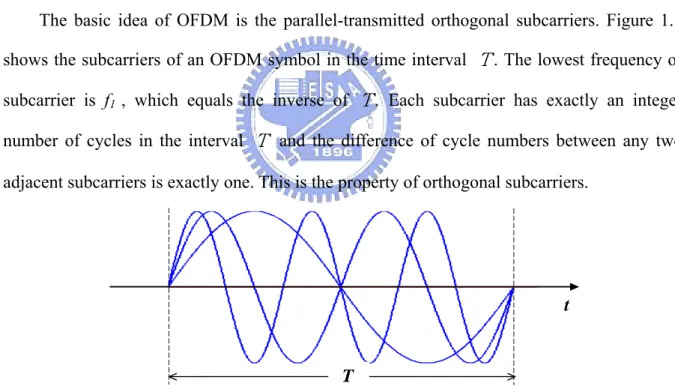
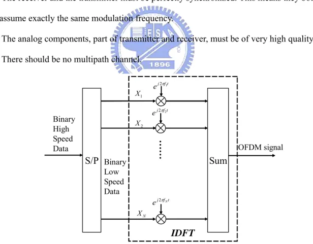
(15) (text, audio, video, etc.). Orthogonal FDM's (OFDM) spread spectrum technique distributes the data over a large number of carriers that are spaced apart at precise frequencies (subcarriers). This spacing provides the "orthogonality" in this technique which prevents the demodulators from seeing frequencies other than their own. The benefits of OFDM are high spectral efficiency, resiliency to RF interference, and lower multi-path distortion. Because of these advantages, OFDM is widely applied in high-speed communication systems. For example : High-speed wire communication systems such as ADSL, VDSL, and XDSL; wireless broadcasting systems such as DAB [5] and DVB [6]；high-speed wireless local area networks (WLAN) such as IEEE 802.11a [3], Hiperlan/2 [15]；OFDM is also the main candidate for the Ultra-Wideband (UWB) systems [4]. The basic idea of OFDM is the parallel-transmitted orthogonal subcarriers. Figure 1.1 shows the subcarriers of an OFDM symbol in the time interval Τ. The lowest frequency of subcarrier is f1 , which equals the inverse of Τ. Each subcarrier has exactly an integer number of cycles in the interval Τ and the difference of cycle numbers between any two adjacent subcarriers is exactly one. This is the property of orthogonal subcarriers.. t. T Figure 1.1 Example of three orthogonal subcarriers of an OFDM symbol. In OFDM the subcarrier pulse used for transmission is chosen to be rectangular. This has the advantage that the task of pulse forming and modulation can be performed by a simple Inverse Discrete Fourier Transform (IDFT) seen in Figure 1.2, which can be implemented 3.

(16) very efficiently as a Inverse Fast Fourier Transform (IFFT) [16]. Accordingly in the receiver we only need a FFT to reverse this operation. According to the theorems of the Fourier Transform, the rectangular pulse shape will lead to a sin(x)/x type of spectrum of the subcarriers. In the Figure 1.3(a) and (b), the frequency interval between any two adjacent subcarriers is f1 and the spectrums of the subcarriers are not separated but overlap. The reason why the information transmitted over the carriers can still be separated is the so called orthogonality relation giving the method its name. By using an IFFT for modulation we implicitly chose the spacing of the subcarriers in such a way that at the frequency where we evaluate the received signal (indicated as arrows) all other signals are zero. In order for this orthogonality to be preserved, the following must be true: 1. The receiver and the transmitter must be perfectly synchronized. This means they both must assume exactly the same modulation frequency. 2. The analog components, part of transmitter and receiver, must be of very high quality. 3. There should be no multipath channel.. X1. e j 2πf1t e j 2πf 2t. Binary High Speed Data. X2. ……. S/P Binary. OFDM signal. Sum. Low Speed Data e j 2πf N t XN. IDFT Figure 1.2 OFDM modulator using IDFT. 4.

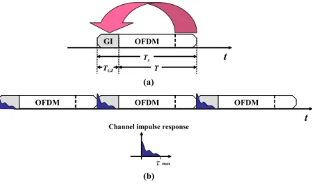
(17) f. f. f1 (a). (b). Figure 1.3 Spectrum of (a) a single sub-channel (b) Orthogonal sub-channels of OFDM systems. In particular the last point is impossible. Fortunately there is an easy solution to deal with multipath delay spread. By dividing the original data stream into several subcarriers, symbol duration extends, which reduces the relative delay spreading. In order to eliminate multipath fading completely, a cyclic prefix (CP) as a guard interval (GI) is introduced after IFFT in OFDM systems. The length of GI is chosen larger than the expected delay spread to avoid ISI. CP is applied to preserve the orthogonality to avoid ICI. The format of OFDM symbol can be shown in Figure 1.4.. GI. OFDM. t. Ts TGI. T. (a) OFDM. OFDM. OFDM. Channel impulse response. τmax. (b). Figure 1.4 (a) a OFDM symbol format (b) ISI caused by multipath fading channel,ΤGI >τmax 5. t.

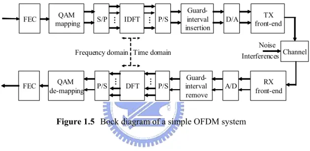
(18) Forward error correction (FEC) is the other main principle of OFDM system. In OFDM transmission, frequency-selective-fading causes different influence on each subcarrier. That is, some data subcarriers may completely be lost due to deep fading, which dominates the overall system performance. FEC is applied to solve this problem. Errors caused by weak subcarriers can be corrected by the coding information. OFDM systems with FEC scheme are often referred as coded OFDM (COFDM) systems. Figure 1.5 shows the block diagram of a general COFDM system.. S/P. IDFT. …. QAM mapping. …. FEC. P/S. Guardinterval insertion. Noise. P/S. DFT. …. QAM de-mapping. …. Frequency domain Time domain. FEC. P/S. TX front-end. D/A. Interferences. Guardinterval remove. A/D. Channel. RX front-end. Figure 1.5 Bock diagram of a simple OFDM system. 1.3. Organization of This Thesis This thesis is organized as follows. In Chapter 2, the simulation platform and detail. specifications of the IEEE 802.11a WLAN, single-band LDPC-COFDM UWB system [17] and the multi-band OFDM-based Ultra-Wideband [8] system will be introduced. Algorithms of the proposed frequency synchronizer for different requirements will be described in Chapter 3 and Chapter 4 respectively. The simulation result and performance analysis will be discussed in Chapter 5. Chapter 6 will introduce the design methodology, hardware architecture, and the chip summary of the proposed design. Conclusion and future work will be given in Chapter 7. 6.

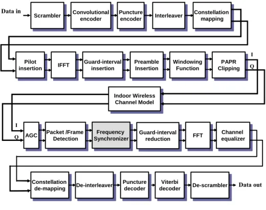
(19) Chapter 2. System Platform In this chapter, we introduce the three system platforms for design analysis and performance simulation. The first one is IEEE 802.11a physical layer (PHY) [3]; the second one is single-band LDPC-COFDM Ultra-Wideband (UWB) system [17]; the other one is IEEE 802.15.3a UWB with multi-band OFDM modulation proposed by Texas Instrument (TI) [4]. The detail block diagram, system specification and preamble format will be described as follows.. 2.1. Introduction to IEEE 802.11a System. 2.1.1. IEEE 802.11a basic. IEEE 802.11a is an OFDM-based indoor WLAN system. The block diagram of the baseband transceiver can be illustrated in Figure 2.1. The system platform includes a COFDM modem and an indoor radio channel model. The COFDM modem comprises a 64-point DFT-based QAM-OFDM modem and a forward-error correction (FEC) coding. The 64 subcarriers contain 48 data carriers and 4 pilot carriers, the others 16 carriers called as null band are set to zero. The OFDM symbol time TS is 3.2µs, the bandwidth of the subcarriers is 1/TS = 312.5 KHz and total bandwidth is N/TS = 20 MHz. The indoor radio channel model comprises a Rayleigh fading channel and AWGN. The supported data rate is from 6Mbits/s to 54 Mbits/s with coding rate equals 1/2, 2/3 and 3/4. The system parameters can be listed in Table 2.1.. 7.

(20) Data in. Scrambler Scrambler. Convolutional Convolutional encoder encoder. Puncture Puncture encoder encoder. Interleaver Interleaver. Constellation Constellation mapping mapping. I Pilot Pilot insertion insertion. IFFT IFFT. Guard-interval Guard-interval insertion insertion. Preamble Preamble Insertion Insertion. Windowing Windowing Function Function. PAPR PAPR Clipping Clipping. Q. Indoor IndoorWireless Wireless Channel ChannelModel Model. I Q. AGC AGC. Packet Packet/Frame /Frame Detection Detection. Constellation Constellation de-mapping de-mapping. Frequency Frequency Synchronizer Synchronizer. De-interleaver De-interleaver. Guard-interval Guard-interval reduction reduction. Puncture Puncture decoder decoder. FFT FFT. Viterbi Viterbi decoder decoder. Channel Channel equalizer equalizer. De-scrambler De-scrambler. Data out. Figure 2.1 System platform of IEEE 802.11a PHY Table 2.1 System parameters of IEEE 802.11a PHY Constellation mapping method BPSK, QPSK, 16QAM, 64QAM Date rate (Mbits/s). 6, 9, 12, 18, 24, 32, 48, 54. FEC coding rate (R). 1/2, 2/3, 3/4. FFT size (N). 64. Number of used subcarriers (NST). 52. Number of data carriers (NSP). 48. Number of pilot carriers (NSD). 4. Bandwidth (MHz). 20. Subcarrier bandwidth (KHz). 312.5 (20 MHz/64). IFFT/FFT period (TFFT). 3.2us. GI duration (TGI). 0.8us (TFFT/4). PLCP preamble duration. 16us (TSHORT + TLONG). 8.

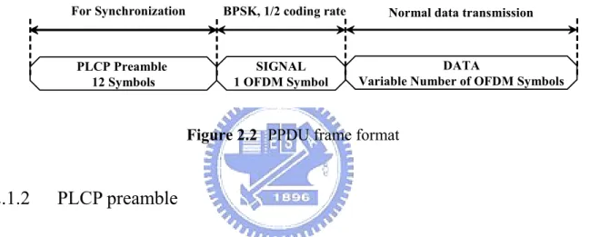
(21) The IEEE 802.11a provides 8 kinds of data rates up to 54 Mb/s by using QAM modulation and convolutional code. The system adopts packet transmission and the PHY protocol data unit (PPDU) frame of IEEE 802.11a shown in Figure 2.2. The PPDU frame format includes the physical layer convergence procedure (PLCP) Preamble, Header and Data fields. The PLCP preamble is a training sequence which is used to perform the synchronization. And the SIGNAL field is always the BPSK modulation and 1/2 coding rate FEC coding. Following the SIGNAL field is the Data field which is used to transmit the general information. For Synchronization. PLCP Preamble 12 Symbols. BPSK, 1/2 coding rate. Normal data transmission. SIGNAL 1 OFDM Symbol. DATA Variable Number of OFDM Symbols. Figure 2.2 PPDU frame format. 2.1.2. PLCP preamble. Figure 2.3(a) shows the structure of the IEEE 802.11a PLCP preamble. The PLCP preamble is composed of 10 identical short symbols and 2 identical long symbols. The short symbol occupies 0.8 µ sec while the long symbol occupies 3.2 µ sec. The total length of the PLCP preamble is 320 samples, each short training symbol contains 16 samples and each long training symbol contains 64 samples. The short symbols serve to do frame detection, automatic gain control, and coarse timing and frequency offset estimation. The two long symbols can be used to do channel estimation and fine CFO estimation. The generation pattern of the short preamble is shown in the left of Figure 2.3(b). These is only one data every four subcarriers. The data carrier spacing is four times larger than the carrier spacing of normal OFDM symbols. The second partition of the PLCP is the long training sequence. It is generated by the pattern in the left of Figure 2.3(c). The right is the sequence of a long 9.

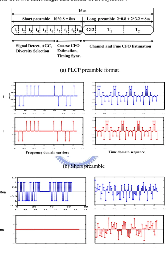
(22) training symbol. The long training sequence contains two repeat OFDM symbols and a guard interval. The GI is two times longer than normal OFDM symbols’. 16us Short preamble 10*0.8 = 8us. Long preamble 2*0.8 + 2*3.2 = 8us. t1 t2 t3 t4 t5 t6 t7 t8 t9 t10 GI2 Coarse CFO Estimation, Timing Sync.. Signal Detect, AGC, Diversity Selection. T1. T2. Channel and Fine CFO Estimation. (a) PLCP preamble format 2. 0.2. 2. 0.2. 1.5. 0.15. 1. 0.1. R e a lp a rt. 1. 0.1. 0.5. 0.05. Real 0. 0. 0. -0.5. -0.05. 0. -1. -0.1. -1. -0.1. -1.5. -0.15. -2 0. -2 0. -0.2. -0.2. 10. 10. 20. 20. 30. 30. 40. 40. 50. 60. 60. 50. 70. 70. 0. 0. 2. 0.2. 1.5. 0.15. 2. 1. 0.1. 0.05. 30. 30. 40. 50. 60. 70. 40. 50. 60. 70. 0.1. 0. 0. -0.5. -0.05. Imag 0. 0. -0.1. -1. -0.1. -1. -0.15. -1.5. -2 0 -2. 20. 20. 0.2. 0.5. 1. 10. 10. -0.2. -0.2. 10. 0. 10. 40. 20. 30. 20. 30. 40. 50. 60. 70. 50. 60. 70. 0. 0. 10. 20. 30. 40. 50. 60. 70. 10. 20. 30. 40. 50. 60. 70. Time domain sequence. Frequency domain carriers. (b) Short preamble 0.2. 1.5 1.5 11 0.5 0.5 00 Real -0.5 -0.5. -1-1 -1.5 -1.5 0 0 1.5 1 0.5 0 Imag -0.5. 0.2. 0.15. 0.1. 0.1. 0.05. 0. 0. -0.05. -0.1. -0.1. -0.15. -0.2. -0.2. 10. 20. 20. 30. 40. 40. 60. 50. 60. 80. 0. 0. 70. 10. 10. 20. 30. 40. 50. 20. 30. 40. 50. 60. 60. 70. 70. 0.2. 0.2. 1.5. 0.15 1. 0.1. 0.1. 0.5. 0.05. 0. 0. 0. -0.05. -0.5. -0.1. -0.1. -1 -1.5 0 -1. -1.5. 0. -0.15. 10. 10. 20. 30. 20. 30. 40. 40. 50. 60. 70. 50. 60. 70. -0.2. -0.2. 0. 0. 10. 10. 20. 30. 40. 20. 30. 40. (c) Long preamble Figure 2.3 PLCP preamble in IEEE 802.11a. 10. 50. 50. 60. 60. 70. 70.

(23) 2.1.3. Transmit Center Frequency Tolerance. In the specification of IEEE 802.11a, the transmitter frequency offset is asked to be small than ±20ppm. If the receiver can achieve the same requirement, the relative frequency between the transmitter and the receiver shall be ±40ppm. The working frequency is about 5.3GHz, the frequency tolerance is ±40ppm. The maximum frequency offset is ±212KHz.. 2.2. Introduction to Ultra WideBand System. 2.2.1. IEEE 802.15.3a UWB basic. OFDM-based wireless ultra-wideband (UWB) technology has received attention from both the academia and the industry. The main reason for the increased attention is the Federal Communications Commission (FCC) allocated 7,500MHz of spectrum (from 3.1GHz to 10.6GHz) for use by UWB devices. It helped to create new standardization, like IEEE 802.15.3a which focuses on developing high-speed wireless communication systems for personal area network. Another reason is because this technology promises to deliver data rates up to 480Mb/s at a distance of 2 meters in realistic multi-path environments. We have established two kinds of UWB systems in platform; one is single-band LDPC-COFDM UWB system [17] which is used low-density parity check (LDPC) FEC codec, the other one is multi-band OFDM-based UWB system [4] which is used convolutional encoder and Viterbi decoder. The block diagram of the UWB PHY is shown in Figure 2.4 which is similar to the IEEE 802.11a WLAN system. The key differences between these two systems can be listed as follow, OFDM symbols are interleaved across both frequency and time. An example of the time-frequency interleaving (TFI) can be shown in Figure 2.5. 11.

(24) From MAC. To MAC. Scrambler Scrambler. QPSK QPSK. Spreading Spreading. IFFT IFFT. Clipping Clipping. Shaping Shaping. Preamble Preamble insertion insertion. Conv. Conv. encoder encoder. RF RFeffects effects. Multipath Multipath. Timing Timing offset offset. AWGN AWGN. DeDescrambler scrambler. Transmitter. LDPC LDPC encoder encoder. Channel Model. LDPC LDPC decoder decoder Viterbi Viterbi decoder decoder. AGC AGC. Timing/Freq Timing/Freq Sync. Sync.. FFT FFT. DeDeQPSK QPSK. DeDespreading spreading. Channel Channel equalizer equalizer. Receiver. Figure 2.4 System platform of UWB PHY The supported data rate is up to 480Mbits/s, which is almost ten times of the data rate in IEEE 802.11a systems. A 128-point FFT is applied and only PSK (BPSK, QPSK) is used in the UWB system. The bandwidth is up to 528MHz, which is 26.4 times wider than IEEE 802.11a.. 9.5 ns Guard Interval for TX/RX Switching Time. 3168 OFDM Symbol #1. Channel 1 3696 Channel 2. 312.5 ns. 4224. 4752. OFDM Symbol #6. OFDM Symbol #3 OFDM Symbol #5. OFDM Symbol #2. Channel 3. 60.6 ns Cyclic Prefix. OFDM Symbol #4. time freq (MHz). Period = 937.5 ns. Figure 2.5 TFI example of the UWB PHY [4] In order to achieve better system performance and higher decoding speed, (600,450) LDPC code is exploited as the kernel of error correcting mechanism in our simulation platform. The parallelism of LDPC decoding makes it easy to decode 480Mb/s data stream or even higher to 12.

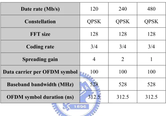
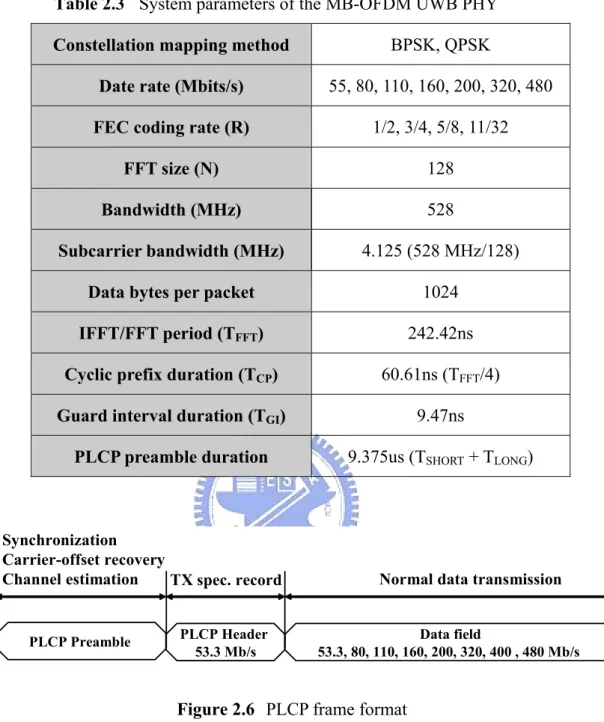
(25) multiple Gb/s. Because of fixed 3/4 FEC coding rate with different spreading gain, we have 120Mb/s, 240Mb/s and 480Mb/s three data-rates. The coding performance can be near Shannon limit when using iterative decoding algorithm. We summarize system parameters about UWB platform that we used in Table 2.2. Table 2.2 System parameters of the LDPC-COFDM UWB PHY Date rate (Mb/s). 120. 240. 480. Constellation. QPSK. QPSK. QPSK. FFT size. 128. 128. 128. Coding rate. 3/4. 3/4. 3/4. Spreading gain. 4. 2. 1. Data carrier per OFDM symbol. 100. 100. 100. Baseband bandwidth (MHz). 528. 528. 528. OFDM symbol duration (ns). 312.5. 312.5. 312.5. The detail specifications of the multi-band OFDM UWB PHY can be listed in Table 2.3. Because of different FEC coding rate with different spreading gain, we have 8 kinds of data-rates. Figure 2.6 shows the format for the PLCP frame including the PLCP preamble, PLCP header and data-field. The PLCP preamble shall be added prior to the PCLP header to aid receiver algorithms related to synchronization, carrier-offset recovery, and channel estimation. The PLCP header is always sent at an information data rate of 53.3 Mb/s. The remainder of the PLCP frame is sent at the desired information data rate of 53.3, 80, 110, 160, 200, 320, 400 or 480 Mb/s.. 13.

(26) Table 2.3 System parameters of the MB-OFDM UWB PHY Constellation mapping method. BPSK, QPSK. Date rate (Mbits/s). 55, 80, 110, 160, 200, 320, 480. FEC coding rate (R). 1/2, 3/4, 5/8, 11/32. FFT size (N). 128. Bandwidth (MHz). 528. Subcarrier bandwidth (MHz). 4.125 (528 MHz/128). Data bytes per packet. 1024. IFFT/FFT period (TFFT). 242.42ns. Cyclic prefix duration (TCP). 60.61ns (TFFT/4). Guard interval duration (TGI). 9.47ns. PLCP preamble duration. 9.375us (TSHORT + TLONG). Synchronization Carrier-offset recovery Channel estimation TX spec. record. PLCP Preamble. Normal data transmission. PLCP Header 53.3 Mb/s. Data field 53.3, 80, 110, 160, 200, 320, 400 , 480 Mb/s. Figure 2.6 PLCP frame format. 2.2.2. PLCP preamble. The signal format of the UWB PLCP preamble is shown in Figure 2.7 and it is different from IEEE 802.11a because of the time interleaving. The preamble contains 30 OFDM symbols, 21 are packet synchronization sequence, 3 are frame synchronization sequences and 6 are channel estimation sequences. The packet synchronization portion of the preamble can be used for packet detection and acquisition and coarse carrier frequency estimation. The 14.

(27) frame synchronization portion of the preamble can be used to synchronize the receiver algorithm within the preamble, and it also provides one sequence period per band with an inverted polarity with respect to the packet synchronization portion of the preamble. Finally, the channel estimation portion of the preamble, denoted as {CE0, CE1, … CE5}, shall be constructed by successively appending 6 periods of an OFDM training sequence. Each OFDM symbol of the UWB contains 32-point pre-GI, 128-point FFT symbol and 5-point post-GI. In IEEE 802.11a system, GI is the cyclic prefix of each OFDM symbols, which is used for the concern of multipath spreading. In UWB system, cyclic prefix (CP) is for multipath concern and the GI is particularly referred to the time between band switching.. 312.5ns 60.61ns. 242.42ns. 9.47ns. 32-point Pre-GI. 128-point FFT Symbol. 5-point Post-GI. (a) OFDM symbol format 9.375us 21 OFDM symbol*312.5ns. PS0. PS1. 3 OFDM symbol*312.5ns. PS20. •••••. Packet Sync. Sequence. FS1. FS0. FS2. Frame Sync. Sequence. 6 OFDM symbol*312.5ns. CE0 CE1. ••••. CE5. Channel Estimation Sequence. (b) Training structure. Figure 2.7 UWB PLCP preamble. 2.2.3. Transmit Center Frequency Tolerance. The MB-OFDM UWB PHY operates in the 3.1~ 10.6 GHz frequency and the relationship between center frequency and band number are given by the following equation: Band center frequency = 2904 + 528 * nb, nb = 1…14 (MHz). This definition provides a unique numbering system for all channels that have a spacing of 528 MHz and lie within the band 3.1~10.6 GHz. Based on this, five band groups are defined, consisting of four groups of three bands each and one group of two bands. Band group 1 is used for Mode 1 devices 15.

(28) (mandatory mode). The remaining band groups are reserved for future use. The frequency of operation form Mode 1 devices is shown in Figure 2.8, and the band allocation is summarized in Table 2.4. In the UWB system, maximum ±20ppm CFO is expected to exist in both transmitter and receiver. So the requested CFO estimation range should be within ±40ppm (TX+RX) of 3.1~10.6 GHz RF frequency. That will be equal ±124KHz~±424KHz.. Band #1. Band #2. Band #3. 3432 MHz. 3960 MHz. 4488 MHz. f. Figure 2.8 Operation frequency for Mode 1 device. Table 2.4 OFDM UWB PHY band allocation Band Group. 1. 2. 3. 4. 5. BAND_ID. Lower frequency (MHz). Center frequency (MHz). Upper frequency (MHz). 1. 3168. 3432. 3696. 2. 3696. 3960. 4224. 3. 4224. 4488. 4752. 4. 4752. 5016. 5280. 5. 5280. 5544. 5808. 6. 5808. 6072. 6336. 7. 6336. 6600. 6864. 8. 6864. 7128. 7392. 9. 7392. 7656. 7920. 10. 7920. 8184. 8448. 11. 8448. 8712. 8976. 12. 8976. 9240. 9504. 13. 9504. 9768. 10032. 14. 10032. 10296. 10560. 16.

(29) 2.3. The Indoor Wireless Channel Model. In order to simulate the data transmission in the real environment, an indoor wireless channel model is established, which includes a time-variant multipath fading [18]-[19], CFO, SCO, and AWGN. The detailed are introduced individually below. 2.3.1. Multipath Fading Channel Model. In wireless communication transmission systems, transmitted signal arrives at receiver through several paths with different time delay and power decay, which is called multipath interference. Figure 2.9 shows the concept of the indoor multipath interference and its channel impulse response and frequency response. The received signal can be modeled as. y (t ) = x (t ) + ∑ β N ⋅ x (t − τ N ). (2-1). N. pulse. Multipaths time. time. Multipaths. Receiver Transmitter. Figure 2.9 Concept of indoor multipath channel. 17. freq.

(30) Due to this effect, the Inter-Symbol Interference (ISI) and frequency-selective fading occur when the maximum delay spread is larger than the symbol period or the channel coherent bandwidth is smaller than the data bandwidth. Although the multipath scales tones, it also remains the orthogonal property because of cyclic prefix technique of each OFDM symbol. The applied multipath fading channel is established according to the IEEE specification. It consists of 13 independent taps, which has Rayleigh distributed magnitude, exponentially decayed power and random uniformly distributed phase [18]. Figure 2.10shows the effect of ISI and frequency-selective fading, and the channel impulse response (CIR) and the channel frequency response (CFR) with RMS delay equals 50ns are shown in Figure 2.11.. Transmitted data. Received data With ISI effect Multipath Without ISI effect. (a) 1.5. 1. 0.5. TX. RX. 0. -0.5. -1. 0 2. 1. 2. Symbol 3. 4. 5. 6. 7. Multipath. 1.4. -1.5. 0. 1. 2. 3. 4. 5. 6. 1.2. 1. 8 0.8. 6 0.6. 4 0.4. 2. 0.2. 0. 0. -0.2. 2. 4 -5. -4. -3. Frequency -2. -1. 0. 1. -0.4 -5. 2. 3. 4. (b). -4. -3. Frequency -2. -1. 0. Figure 2.10 (a) ISI effect (b) frequency-selective fading channel. 18. 1. 2. 3. 4.

(31) 0.35. CIR Magnitude. CFR Magnitude. 0.3. 1. 0.25. 0.8. 0.2. 0.6. 0.15. 0.4. 0.1. 0.2. 0.05. 0. 0 0. 15 10 5 RMS Delay Spread [100ns]. -0.2 0. 20. 60 40 20 Subcarrier Index [312.5KHz]. 80. (b). (a). Figure 2.11 (a) CIR (b) CFR example of the multipath fading channel. 2.3.2. Carrier Frequency Offset Model. The sensitivity to carrier frequency offset (CFO) is one of the main drawbacks of the OFDM system. One of the reasons causing the CFO in wireless communication is the RF circuit mismatch between the transmitter and the receiver. When the transmitter carriers the data xt with a frequency f1 (2.2) and the receiver gets the data with another frequency f 2 (2.3), the received data yt contains the original data and a sinusoidal signal with a frequency f1 − f 2 .. T = xte −. j 2 π f1t. (2.2). y t = Te j 2 πf 2 t = x t e − j 2 π ( f 1 − f 2 ) t. (2.3). Another reason caused the CFO is the Doppler Effect. From the Doppler equation (2.4), the received signal will not equal to the transmitted one if the relative speed between the transmitter and the receiver is not zero. There will be some frequency offset fδ existed. Because of the v is the velocity of light, the fδ is usually negligible as compared with the CFO caused by the circuit mismatch. 19.

(32) f ′ = f0. v ± vr v ± vt. (2.4). fδ = f ′ − f0 = f0. ± vr µ vt v ± vt. (2.5). No matter the causes of the CFO, the behavior of the CFO in the spectrum domain is shown in the Figure 2.12. The total frequency offset is f1-f2+fδ and it will be expressed as f∆ in the thesis. Besides, the orthogonal property between each subcarrier is based on the perfect sampling on some specific frequencies in the spectrum domain. When we transmit the data without CFO, the received data will be recovered perfectly because of the influences from others subcarriers’ are all zero, which shown in Figure 2.14(a). The equation (2.6) and (2.7) are the N points IDFT and DFT equation. The x n and X k in the (2.6) are the data of time domain and frequency domain, respectively.. F N− 1 {X k } = x n = F N {x n } = X. k. 1 N =. N −1. ∑. k=0. N −1. ∑. n=0. X k e 2 π jkn / N , k = 0 ,1 , 2 ,... N − 1. x n e − 2 π jkn. / N. , n = 0 ,1 , 2 ,... N − 1. TX. (2.6) (2.7). f1. Channel f2. RX. f1+fδ. f1+fδ-f2. Figure 2.12 The behavior of the CFO in spectrum domain Applying equation (2.3) to discrete time, if there is no CFO within transmission, the received data yn is equal to the transmitted data xn . The received data Yk in the frequency domain are the same with the transmitted data X k .. 20.

(33) Yk = =. N −1. ∑. n=0. N −1. ∑. n=0. y n e − 2 π jkn ⎧ 1 ⎨ ⎩ N. N. k=0. ∑. n=0. N −1. ∑. N −1. =. X ke. x n e − 2 π jkn. 2 π jkn / N. ⎫ − 2 π jkn ⎬e ⎭. /N. (2.8) /N. = X. k. However, the data can not be received perfectly in the CFO environment. In the time domain, the received data suffering from CFO is shown as equation (2.9), where Ts is the sampling time and the 1/NTs is the subcarrier bandwidth of an OFDM symbol. We normalize the frequency offset f∆ to the subcarrier bandwidth and ∈ is the relative frequency offset. y n = x n e − j 2 π tf ∆ = x n e − j 2 π nT s f ∆ = x n e − j 2 π n ( NT s ) f ∆ / N = x n e − j 2 π n ∈ / N. (2.9). From the publish of Moose [14], the CFO caused linear phase shift in time domain will convert to ICI in the frequency domain after passing the DFT, which shown in Figure 2.13 and Figure 2.14(b) respectively, and the relative equation is shown in (2.10). Yk =. N −1. ∑. n= 0. y n e − 2πjkn / N =. Yk = X k e +. j π ∈( N − 1 ) / N. N −1. ∑X eπ. l = 0,l ≠ k. N −1. ∑ye n=0. ⋅ {[sin( π ∈) ] / N [sin( π ∈) / N ]}. j ∈( N − 1 ) / N. l. − 2 πj ( k + ∈ ) n / N. n. ⋅ e − jπ ( l − k ) / N ⋅{[sin( π ∈) ] / N [sin π ( l − k + ∈) / N ]}. Figure 2.13 Linear phase shift. 21. (2.10).

(34) Perfect sampling point. imperfect sampling point. frequency. frequency. (a). (b). Ideal. With CFO. Figure 2.14 The received data (a) without CFO (b) with CFO (ICI). In order to simulate the real CFO environment, we find a phase noise model such as Figure 2.15. According to this phase noise model, we built it in our platform. Figure 2.16 shows the example of phase noise which normal distributed with 40ppm (400 KHz) mean-CFO. In general, the mean CFO is time-invariant. However, in order to consider about more complete simulation condition, we define the mean CFO could be time-variant. We defined three kinds of CFO environments, the first one is time-invariant (TIV), and the second one is slow-variant (SV) which changed 80ppm within 50ms, and the final one is fast-variant (FV) which changed 80ppm within 5ms. Figure 2.17 shows the three CFO definitions of TIV, SV and FV. These definitions are helpful for explanation of following design.. 22.

(35) 0 -10 -20. PSD (dB c/H z). -30 -40 -50 -60 -70 -80 -90 -100 1.E-01. 1.E+00. 1.E+01. 1.E+02. 1.E+03. 1.E+04. 1.E+05. Frequency(Hz). Figure 2.15 Phase noise model. +15Hz. 4.0001. x 10. 5. +10Hz. CFO. 4.0001. +5Hz. 4. 400KHz. 4. -5Hz. 4. -10Hz. 3.9999. -15Hz. 3.9998. 0 0. 0.5. 2. 1. 4. 1.5. 6. 2. 8. 2.5. 10. 3. 12. 3.5. 4. 4.5. 5. 14 16 18 20 x 10. 4. Time [μs]. Figure 2.16 Example of phase noise. 40ppm. TIV -40ppm. 1s 40ppm. SV. 50 ms. -40ppm 40ppm. FV. 5 ms. -40ppm. Figure 2.17 Mean CFO definition 23.

(36) 2.3.3. Sampling Clock Offset Model. Sampling Clock Offset (SCO) is the sampling clock rate mismatch between the digital to analog converter (DAC) in transmitter and the analog to digital converter (ADC) in receiver. In the platform, the model of clock offset is built using the concept of interpolation. The input digital signals and the shifted sinc wave can interpolate the value between two sampling points. The received signal after ADC can be derived as equation (2.11).. R(nTs ) = R preADC (nTs ) ∗ sinc(. nTs − ∆Pn ) Ts. (2.11). ∆P = ∑ R preADC (nTs − kTs ). sinc(k − n ) Ts k =− l l. Where R(nTs ) is output signal of ADC and l is the sampling point index. Because of the SCO, even if the initial sampling point is optimized, the following sampling points will slowly shift with time. This shift in time-domain becomes a phase rotation in frequency-domain. Figure 2.18 shows the time-domain oversampled received data and the frequency-domain linear phase shift caused by SCO. 6 5 4. Phase [dB]. 3 2 1 0 -1 -2 Original Oversampled Oversampled+clock offset. -3 -4 0. 1. 3 2 Symbol [50ns]. 4. 5. Subcarrier 6. (a). (b). Figure 2.18 (a) the time-domain sampling offset (b) the frequency-domain linear phase shift 24.

(37) 2.3.4. AWGN Model. The AWGN channel model is established by the random generator in Matlab. The output random signal is normally distributed with zero mean and variance equal to 1. The complex AWGN noise can be modeled as. w (t ) = [randn(1, l ) + j ⋅ randn(1, l )] ⋅. 10. PS − SNR 20. 2. (2.12). Where PS is the data signal power, SNR is the signal to noise power ratio, and l is the data signal length.. 25.

(38) Chapter 3. A Frequency Synchronizer Design for OFDM WLAN Systems As for the complement to periodic and non-constant-power preamble in IEEE 802.11a, low-complexity frequency estimators are of interest. Such estimator is relied on the phase information of auto correlations. In this chapter, we chose fewer samples for auto correlation based on the average power of preamble before FFT process. We also derive the performance and show how the correlation samples should be properly chosen with acceptable SNR loss.. 3.1. Carrier Frequency Offset Synchronization For packet-based OFDM wireless systems, the burst synchronization is needed. We. generally used data-aided methods which inserted the special synchronization information to estimate the CFO. The data-aided CFO estimation can achieve the system requirement in a very short time period.. 3.1.1. The algorithms of CFO estimation and compensation. In the 1994, Paul H. Moose [14] proposed a method to estimate frequency offset from the demodulated data signals in the receiver. This method involves repetition of a data symbol and compares the phases of each of the carriers between the successive symbols. Since the modulation phase values are not changed, the phase shift of each of the carriers between successive repeated symbols is due to the frequency offset. If an OFDM transmission symbol is repeated, one receives, in the absence of noise, the 26.

(39) received training symbol rn that interfered by CFO ∈ is shown in (3.11), and –K…K are subcarriers’ indexes.. rn =. 1 N. K. ∑X. k=− K. k. H k e 2 πj ( k +∈ ) n / N ; n = 0,1,..., 2 N − 1. (3.11). The kth elements of the N point DFT of the first and second N points of (3.11) are shown in (3.12) and (3.13) respectively.. R1 k = R2k =. N −1. ∑re. − 2 π jnk / N. n. n=0. 2 N −1. ∑. n= N. rn e − 2 π jnk. /N. ; k = 0 ,1 , 2 ,..., N − 1 =. N −1. ∑r n=0. n+ N. e − 2 π jnk. /N. ; k = 0 ,1 ,... N − 1. (3.12) (3.13). From (3.11), we know that rn + N = rn e 2 πj∈ and the R2 k becomes (3.14). R2 k =. N −1. ∑re n= 0. n. 2 π j∈. e − 2 π jnk / N = e 2 π j∈ ⋅ R1 k. (3.14). Including the AWGN as below, Y1k = R1k + W 1k Y 2 k = R 1 k e 2 π j∈ + W. 2k. ; k = 0 ,1 ,..., N − 1. (3.15). Both the ICI and the signal of the first and second observations are altered in exactly the same way, by a phase shift proportional to frequency offset. Therefore, the offset ∈ will be estimated using observations (3.15) is shown in (3.16). ⎧⎛ K ⎞ ˆ = (1 2π ) tan − 1 ⎨ ⎜⎜ ∑ Im[Y2 kY1∗k ] ⎟⎟ ∈ ⎠ ⎩⎝ k = − K. ⎞⎫ ⎛ K ⎜⎜ ∑ Re[Y2 kY1∗k ] ⎟⎟ ⎬ ⎠⎭ ⎝ k=−K. (3.16). This algorithm, however, can only correctly distinguish the phase rotation in the range [-π, π], the estimation limitation is shown in equation (3.17). In (3.17) and (3.18), the NTs means the time interval between the two repeat symbols. Minimizing the interval time to the OFDM symbol time can make the maximum CFO estimation range to be half of the subchannel bandwidth. According to the (3.18), the method to get a larger CFO estimation range is to shorten the training symbol time. The idea is also suggested in the [14]. 2π ∈ = 2πNTs f ∆ ≤ π. (3.17) 27.

(40) f∆ ≤. 1 2 NTs. (3.18). After finishing the acquisition of CFO, we counteract the frequency offset that we estimated to compensate the following complex data signal as equation (3.19). rˆk = rk ⋅ exp( − j 2π ∈ˆ kT ); k = 0 ,1 , 2 ,.... (3.19). Where rk are the received complex signals that influenced by CFO ∈ and k are the indexes of data signal.. 3.1.2. The structure of CFO estimation and compensation. The training symbols are provided for burst synchronization in the packet-based transmission system. As previous discussion in section 3.2.1, the repeated OFDM symbols can be used to perform the CFO synchronization. One reason we using time domain estimation and compensation is that the frame detector can get a less distortion training pattern to judge the frame boundary more accurately. The other one is that the compensated training data can be used to estimate the channel response directly by the channel equalizer after FFT process. In order to cover a larger CFO estimation range, we need two stages CFO estimation as Figure 3.1 by means of short and long symbols in the preamble. According to the properties of short and long training symbols, coarse CFO estimation gets a rougher estimate under a wider frequency offset range while fine CFO estimation gets narrower but more accurate results. Taking advantages of both estimation results in a more precise estimate for CFO under a wider CFO range. Basing on the IEEE 802.11a specification, the maximum tolerance center frequency offset of the transmitter and the receiver shall be within ±40ppm of 5.3 GHz RF frequency; that is equal to ±212 KHz; and further, due to the 0.8µs short and 3.2µs long training preamble provided for coarse and fine CFO estimation, the enduring estimation range 28.

(41) are about -118ppm ~ 118ppm (-625KHz ~ 625KHz) and -30ppm ~ 30ppm (-156.25KHz ~ 156.25KHz) respectively.. Received data. Coarse CoarseCFO CFO compensator compensator. Fine FineCFO CFO compensator compensator. FFT Coarse CoarseCFO CFO estimator estimator. Fine FineCFO CFO estimator estimator. Figure 3.1 The structure of two stages CFO synchronization In the acquisition scheme, coarse and fine CFO estimations and compensations are performed by using the same algorithms. The coarse CFO estimation is available from equation (3.20).. ⎤ ⎡ N s −1 Im ∑ rn ⋅ rn∗+ N s ⎥ ⎢ 1 ⎥ ˆ coarse = tan −1 ⎢ Nns=−01 ∈ 2πTs ⎥ ⎢ ∗ ⎢ Re ∑ rn ⋅ rn+ N s ⎥ n= 0 ⎦ ⎣. (3.20). Where Ts is short training symbol period; that is 0.8µs; and Ns is the number of samples in a short training symbol. Before fine CFO estimation, the long training symbols shall be compensated with the frequency estimated as equation (3.21). rˆk , long = rk , long ⋅ exp( − j 2π k ∈ˆ coarse T ); k = 0 ,1, 2 ,... 127. (3.21). Where k is index of long training symbol, and T is sample period that equal to 1/20MHz. Therefore the fine CFO estimation is represented as equation (3.22). ⎤ ⎡ N L −1 Im ∑ rn ⋅ rn∗+ N L ⎥ ⎢ 1 ⎥ ˆ fine = tan −1 ⎢ NnL=−01 ∈ 2πTl ⎥ ⎢ ∗ ⎢ Re ∑ rn ⋅ rn+ N L ⎥ n= 0 ⎦ ⎣. (3.22). Where Tl is long training symbol period; that is 3.2µs; and NL is the number of samples in a long training symbol. After finishing the acquisition of CFO, both coarse and fine estimation is available. The 29.

(42) following complex data signals including of long symbols, header and payload shall be compensated by estimated coarse and fine CFO as equation (3.23) and rk is the complex signal beginning from long symbols. rˆ k = rk ⋅ exp[ − j 2π k (∈ˆ coarse + ∈ˆ fine )T ]; k = 0,1, 2,.... 3.2. (3.23). The Proposed CFO Estimation Scheme In a real system, several synchronization issues must be taken care including frame. detection, multipath cancellation and other channel effects. The only purpose that we considered in low-complexity method is trying to reduce the number of correlations as far as we keep the performance of CFO estimation. We analyze the average-power distribution of preamble in IEEE 802.11a, and decided which points of preamble we used for complex multiplier to estimate the CFO.. 3.2.1. Property of Preamble. According to the specification of IEEE 802.11a, besides the format of preamble, the signals which carried by the preamble are non-constant power. In other words, the power distribution of each sample in the short and long training symbols is different; it also affects the accuracy of the following frequency synchronization. Therefore, we analyze the power distribution of the time-domain preamble under both AWGN and multipath fading channel as Figure 3.2. Because AGC and packet detection need to take several short training symbols before coarse CFO estimation, we use four short symbols and two long symbols for power analysis. We separate the index of samples of short and long training symbols into two parts; one is even index of samples, the other is odd one; and sum their power respectively. From Figure 3.2(a) and (b), the z-axis represents the probability that the odd-index power larger even-index one, and we can obviously see that the results from short and long training 30.

(43) symbols are opposite and they also be influenced graver by multipath effect.. 3.2.2. Samples Power Detection. For low complexity method, we can reduce the half samples of short and long training symbols for correlations according to the information of even or odd index from power distribution of samples. In the realistic system, we need the packet detection before the CFO acquisition. Nevertheless, even if we have packet detection, we can not ensure how accurate is; furthermore, because of the multipath effect, the power distribution of samples in the short and long training symbols could be changed probably in the same time. For these reasons, we take one more short-symbol to detect the next coming short symbols which samples have stronger power. Due to one short symbol includes 16 samples, and we sum each sample power of even and odd index respectively. And then we can determine that even or odd index samples have stronger power for coarse CFO estimation. Certainly, the opposite result of the detection can be used for following fine CFO estimation. Therefore, the algorithms of the coarse and fine CFO estimation can be modified as equation (3.24) and (3.25) respectively; and λ is decided by sample power detector. Consider about limited short training symbols and the performance trade off, we used twice correlations that total three short symbols needed. Figure 3.3 shows the synchronization flow with the sample power detection and the interactive between the packet detection and CFO compensation before FFT demodulation. ⎤ ⎡ N s 2 −1 ⎢ Im ∑ r2 n+ λ ⋅ r2∗n+ λ + N ⎥ s 1 ⎥ ⎢ ˆ coarse = tan −1 ⎢ Nns =0 ∈ ⎥; λ = 0(even),1(odd ) − 1 2πTs 2 ⎢ Re r2 n+ λ ⋅ r2∗n+ λ + N s ⎥⎥ ∑ ⎢⎣ n= 0 ⎦. (3.24). ⎤ ⎡ N L 2 −1 ⎢ Im ∑ r2 n+ λ ⋅ r2∗n+ λ + N ⎥ L 1 ⎥ ⎢ ˆ fine = tan −1 ⎢ NnL=0 ∈ ⎥ ; λ = 0(even),1(odd ) 2πTl 2 −1 ⎢ Re r2 n+ λ ⋅ r2∗n+ λ + N L ⎥⎥ ∑ ⎢⎣ n= 0 ⎦. (3.25). 31.

(44) Pr( odd-index power > even-index power). Probability [%]. *Sim ula. SNR. ted p. [dB]. acke. t s pe. r SN R:1. 00 00. ] RMS [ns. (a) Pr( odd-index power > even-index power). Probability [%]. *Simula ted pac k. ets per. SNR :. 100000. [ RMS. SNR [dB ]. ns]. (b). Figure 3.2 Power distribution of (a) Short training symbols (b) Long training symbols. 32. 0.

(45) Received Receiveddata data. No. Short Shorttraining training Symbol Symbolstart? start? Sample Samplepower powerdetection detection. Yes Coarse CoarseCFO CFOestimation estimation and compensation and compensation Detect Detectlong longtraining trainingsymbol symbol and andfine fineCFO CFOestimation estimation No. Even/Odd Odd/Even. Long Longtraining training Symbol Symbolstart? start? Yes Fine FineCFO CFOcompensation compensation. FFT FFT. Figure 3.3 The synchronization flowchart with sample power detection. 33.

(46) Chapter 4. A High Speed and Low Complexity Frequency Synchronizer for OFDM-based UWB System For general OFDM-based wireless access systems, we proposed a frequency synchronizer in chapter 3. Based on this design, the modifications can be made when dealing with different applications with particular requirements and specifications. In this chapter, a high-speed and low complexity frequency synchronizer is proposed for 528MHz OFDM-based UWB system.. 4.1. Motivation To speed up the implementation and power-reduction of 528MHz UWB frequency. synchronizer, a novel low-power scheme combining data-partition-based, power-aware CFO estimation and approximate phasor compensation is proposed. It can reduce redundant computation of synchronization algorithm according to performance requirement. Following the algorithm improvement, the needed memory and clock speed of frequency synchronizer can be both decreased. In the further, we can reduce more power consumption in the better channel condition by power-aware concept. Simulation results show the power elimination efficiency is 69.4 ~ 75.6% and the paid performance loss can be limited to 0.04 ~ 0.6dB for typical 8% packet-error-rate (PER) for UWB.. 4.2. Effect of Carrier Frequency Offset In UWB system, maximum ±20ppm CFO is expected to exist in both transmitter and 34.

(47) receiver. So the required CFO estimation range must be ±40ppm (TX+RX) in frequency synchronizer. Besides, in order to enhance system performance, an accurate CFO estimation is generally requested in frequency synchronizer. However as system migrates from WLAN to UWB, the performance degradation caused by CFO becomes different. According to [14], the average power of frequency-domain signal without inter-carrier interference (ICI) can be derived as equation (4.1).. [ ]= X. E YK. 2. 2. H {[sin π ∈] [ N sin(π ∈ N )]} 2. 2. (4.1). Where YK is the received signal, |X|2 is the average transmitted signal power, |H|2 is the average channel response power, ∈ is the relative CFO of the channel (the ratio of actual CFO to the subcarrier spacing), and N is the point number of the DFT used for OFDM. In the (4.1), it can be found that the signal power is degraded by relative CFO ∈. The CFO also causes ICI which is added to the received signal. According to [14], the average power of ICI can be derived as equation (4.2).. [ ]= X. E IK. 2. 2. H {sin π ∈} 2. 2. K −k. ∑1 {N sin[π ( p + ∈). N ]}. 2. (4.2). p =− K −k p ≠0. Where IK is the ICI of the OFDM system, which using 2K+1 subcarriers. From (4.1) and (4.2), the signal-to-ICI ratio (SIR) of UWB and WLAN system can be calculated and then drawn in Figure 4.1. Since the specifications containing subcarrier spacing, RF frequency, and subcarrier number of UWB and WLAN system are different, the SIR of UWB is ~18dB higher than that of WLAN. The main cause is that the subcarrier spacing of UWB (4.125MHz) is 13.2 times wider than that of WLAN (312.5 KHz). Therefore the relative CFO ∈ of UWB becomes lower. The lower relative CFO leads to less performance degradation. To understand the required CFO-estimation accuracy from a system-level view, we simulated baseband PER with different CFO-estimation error. The simulated SNR loss for 8% PER caused by CFO-estimation error is shown in Figure 4.2.From Figure 4.2, it is found the 35.

(48) tolerant CFO-estimation error of UWB can be higher than of WLAN in the same SNR-loss constraint. For example, in 1dB SNR-loss constraint, the estimation error of UWB can be tolerated to 5ppm, but the estimation error of WLAN must be lower than 0.4ppm. Based on the performance comparison, the required accuracy and design complexity of CFO estimation in UWB can be less than that in WLAN. And a low-power scheme with algorithm reduction can be exploited in frequency synchronizer.. Signal-to-ICI ratio [dB]. 50. 45. IEEE 802.11a system in 5.8GHz RF band UWB system in 10.6GHz RF band. 40. 35. 30. 25. 20. 15. 10 2. 4. 6. 8. 10. CFO estimation error [ppm]. Figure 4.1 Signal-to-ICI ratio under CFO effect. SNR Loss for 8% PER [dB]. 8 7. 480Mb/s UWB system @ 10.6GHz RF 54Mb/s IEEE 802.11a system @ 5GHz RF. 6 5 4 3 2 1 0 0. 2. 4. 6. 8. 10. CFO [ppm] ＊Simulated packets per SNR: 1500, Data bytes per packet: 1024. Figure 4.2 SNR loss caused by CFO estimation error 36.

(49) 4.3. The Proposed CFO Estimation and Compensation Scheme The Figure 4.3 shows the block diagram of the proposed frequency synchronizer. In the. beginning, the received preamble is sent to CFO estimator. Then the estimated result is sent to CFO compensator. And the late preamble and data signal are compensated and sent out. The compensated output signal can be used for timing synchronization and data demodulation. Besides, the proposed design is developed based on a data partition scheme in CFO estimator and an approximate phasor compensation scheme in CFO compensator to reduce design complexity. The proposed low-complexity algorithms will be described below.. Estimated result. CFO Estimator. Preamble. From ADC. Preamble and data. CFO Compensator. To FFT. To Symbol-timing detector. Figure 4.3 Block diagram of frequency synchronizer. 4.3.1. Data-partition-based CFO Estimation. The conventional CFO estimator algorithm which uses full repeated symbols for auto-correlation is derived as equation (4.3).. 37.

(50) N −1 ⎧ Im rn ⋅ rn∗+ N ∑ ⎪⎪ 1 n= 0 tan −1 ⎨ ∈ˆ = N −1 2π NT ⎪ Re ∑ rn ⋅ rn∗+ N ⎪⎩ n=0. ⎫ ⎪⎪ ⎬ ⎪ ⎪⎭. (4.3). ˆ is the estimated CFO, rn is the n-th received sample, and N is the total sample Where ∈ amount of one symbol. So r0 ~ rN-1 are the samples of one symbol duration. In UWB system, N is equal to 165 for repeated OFDM symbols [8]. And in CFO estimator, the first symbol with N samples needs to be stored in memory or delay-line [9]. To reduce the required memory access, a low-power algorithm based on data partition is proposed. It can be derived as equation (4.4).. ⎣N λ ⎦− 1 ⎧ ⎪ Im ∑ rλ n ⋅ rλ∗n + 3 N 1 ⎪ n=0 ∈ˆ = ⎨ ⎣N λ ⎦− 1 6 π NT ⎪ ∗ ⎪ Re ∑ rλ n ⋅ rλ n + 3 N n=0 ⎩. ⎫ ⎪ ⎪ ⎬ ⎪ ⎪ ⎭. (4.4). Where the used samples of the first repetitive symbol duration are r0, rλ, r2λ, r3λ, …, and r( ⎣N ⎦− 1 )× λ ,which are just ⎣ N λ ⎦ samples. In the proposed CFO estimation algorithm, the λ. used sample amount is reduced from N to ⎣ N λ ⎦ , which shown in Figure 4.4. Therefore, the design complexity of auto-correlation containing the memory size to store the used samples and the multiplication of used samples can be efficiently reduced. Besides, the different correlation distance will affect the estimation accuracy and range. The signal power of image part will be increased because of long correlation distance, and then the estimation accuracy will be improved. However, the long correlation distance also decreased the estimation range. For the estimation accuracy and range trade off, the correlation distance is limited to 3NT, that equal to 0.9375µs. So the estimation range can achieve ±0.5/0.9375µs = ±533KHz [14], that is ±50.3ppm of the highest RF frequency (10.6GHz) of UWB system. Thus the proposed algorithm can meet the requested ±40ppm CFO estimation range. Coincident, the 3NT correlation distance also can be applied in the 38.

(51) multi-band UWB system [4], for example, used time-frequency code 1 for band group 1, where the first OFDM symbol is transmitted on sub-band 1, the second OFDM symbol is transmitted on sub-band 2, the third OFDM symbol is transmitted on sub-band 3, the fourth OFDM symbol is transmitted on sub-band 1, and so on. This concept of the correlation distance also shown in Figure 4.4(b).. r0. r1. r2. r3. rN* rN+1 * rN+2* rN+3*. rN-2 rN-1. r2N-2 * r2N-1 *. Received signal: Required ??. Tan-1. (a). Received signal: r0. r1. r2. Multiplication: λ. r3. * r3N * r3N+1 * r3N+2 * r3N+3. rN-1. r4N-1 *. 1. Tan-1. (b) Figure 4.4 (a) The conventional CFO estimation (b) The proposed data-partition-based CFO estimation In order to reduce complexity and keep performance simultaneously, we have to find a good λ value. As Figure 4.5 shown, if high λ value is chosen, the complexity will be lower, but the CFO estimation error will be increased. In the section 4.3.3, we will choose a good λ value according to the performance loss.. 39.

(52) 8. Low λ: High complexity Low estimation error. 6. RMSE [ppm]. High λ: Low complexity High estimation error. lamda λ= 1 =1 lamda λ= 2 =2 λ= 4 Proposed: lamda = 4 λ= 8 =8 lamda λ= 16 lamda = 16. 7. 5 4 3 2 1 0 0. 5. SNR [dB]. 10. 15. Figure 4.5 CFO estimation error with different complexity. 4.3.2. Approximate phasor Compensation. In compensation part, the ideal method is to directly compensate the received signal with the phasor. It can be derived as equation (4.5). rˆk = rk ⋅ exp( − j 2π ∈ˆ kT ). (4.5). ˆ is the estimated CFO, T is the sample period, Where rk is the k-th received sample, ∈ ˆ kT ) is the compensating value, and rˆk is the compensated sample. In UWB exp(− j 2π ∈ system, the sample period (T=1/bandwidth=1/528MHz) is shorter than 1.9ns. So the compensating phasors for neighboring samples are approximate to each other. Hence the proposed approximate compensation scheme is derived as equation (4.6). ⎢k ⎥ ˆ ⎢ ⎥ λT ) rˆk = rk ⋅ exp(− j 2π ∈ ⎣λ ⎦. (4.6). ˆ ⎣k λ ⎦λT ) is the compensating phasor, and it remains the same for λ Where exp(− j 2π ∈. samples. For example, the phasors for r0 ~ rλ-1 are the same and equal to exp(j0) = 1 since. ⎣k λ ⎦ with k = 0 ~ λ-1 are all equal to 0; and the Figure 4.6 shows this example of the proposed algorithm where λ = 4. So each phasor can be used to compensate λ samples. And the phasor computations of (4.6) can be reduced to ~ 1/λ of that of (4.5). Figure 4.7 shows the examples which are the real parts of compensating phasor of (4.5) and (4.6) with λ = 4 and 40.

(53) ˆ = 424 KHz (40pm of 10.6GHz). And the x-axis is the receiving time (kT). As shown in ∈ Figure 4.7, the difference between the real parts of compensating phasor can be less than 2%. The difference is small so the approximate phasor compensation can be used to reduce the phasor computations. Received data: r0 θ0. r1 θ1. r2 θ2. r3 θ3. r4 θ4. r5. r6. θ5. θ6. r7 θ7. r8 θ8. r9 θ9. r10. r11. θ10 θ11 Required ??. rˆ0 rˆ1 rˆ2 rˆ3 rˆ4 rˆ5 rˆ6 rˆ7 rˆ8 rˆ9 rˆ10 rˆ11 (a) Received data: r0. LUT complexity λ. 1. r1. r2. θ0. r3. r4. r5. r6. r7. θ4. rˆ0. r8. r9. r10. r11. θ8. rˆ1 rˆ2 rˆ3 rˆ4 rˆ5 rˆ6 rˆ7 rˆ8 rˆ9 rˆ10 rˆ11 (b). Figure 4.6 CFO compensation scheme (a) Conventional approach (b) Proposed approach. <2%. 600. 610. 620. 630. 640. 650. Figure 4.7 Real parts of compensating phasor 41. 660.