投資型金融商品與退休金制度附加最低保證之評價

行政院國家科學委員會

獎勵人文與社會科學領域博士候選人撰寫博士論文

成果報告

投資型金融商品與退休金制度附加最低保證之評價

核 定 編 號 ： NSC 95-2420-H-002-032-DR 獎 勵 期 間 ： 95 年 08 月 01 日至 96 年 07 月 31 日 執 行 單 位 ： 國立臺灣大學財務金融學系暨研究所 指 導 教 授 ： 楊曉文 博 士 生 ： 唐俊華 公 開 資 訊 ： 本計畫可公開查詢

中 華 民 國 96 年 08 月 07 日

國立臺灣大學管理學院財務金融學系

博士論文

Department of Finance

College of Management

National Taiwan University

Doctoral Dissertation

附收益率保證確定提撥制退休金計畫之研究

The Study of Rate of Return Guarantees

under Defined Contribution Pension Plans

唐俊華

Tang, Chun-Hua

指導教授：曾郁仁博士、楊曉文博士

Advisors: Tzeng, Larry Y., Ph.D.

Yang, Sharon S., Ph.D.

中華民國 96 年 6 月

June, 2007

謝 辭

從踏入台大的第一天算起，經歷大學部、碩士班、博士班，至今已有十四年， 這段時間受到許多人的幫助。感謝我的家人，由於父親母親與姊姊的栽培及支 持，讓我在學習過程中，能夠專心於學業，並且順利完成博士學位。感謝台大財 金所提供多元課程與豐富資源，讓我學習到財務金融、財務工程以及退休金領域 的知識，並且結合於博士論文中。感謝博士論文指導教授－曾郁仁老師與楊曉文 老師，謝謝曾老師的協助，更謝謝楊老師在研究過程中給予諸多指點，讓我在學 術的道路上不斷成長。感謝廖咸興老師、蔡政憲老師與謝明華老師的建議，讓我 的博士論文更加完善。感謝曾經教過我的所有老師，尤其是葉小蓁老師、陳業寧 老師、巫和懋老師，幫助我在修課過程中建立紮實的研究基礎。感謝林煜宗老師、 林筠老師、岳夢蘭老師，謝謝您們給予我在生活上或研究上的幫助。感謝多位學 長姊以及博士班的同班同學們，謝謝你們讓我在修課與資格考過程中，有請益與 切磋的對象。感謝國科會的獎勵，讓我在博士班的第五年能夠專心致力於撰寫論 文。更要感謝上天的保祐，讓我的人生旅程能順利進展。 在接下來的人生中，期望自己能夠將所學貢獻給社會，並且盡一己之力幫助 需要幫助的人，存好心、說好話、做好事。與大家共勉之。

中文摘要

本論文包含兩篇文章，皆是以附收益率保證確定提撥制退休金計畫為研究主 軸。第一篇文章推導附收益率保證之評價公式，此收益率保證乃是連結至年期 定存利率，並且兼具互換選擇權、路徑相依選擇權、遠期生效選擇權之性質。本 文同時考慮兩種保證型態：到期日保證與多期保證，運用平賭訂價理論以及 Margrabe (1978)的方法，在一因子 HJM 利率模型下推導這兩種保證的價格公式 解，並且分析重要參數對價格的影響。第二篇文章延續第一篇的保證型態，分析 投資策略與行為是否會影響保證成本與退休金收益。本文假設利率動態遵循 CIR 模型，並設定買進持有策略與多種更換投資組合策略，以模擬方式得到保證成本 與退休金收益的數值結果。在本文的保證型態與參數設定下，計畫參與者可以買 進具有高報酬率與高波動率的投資組合並持有至退休日，以獲得高預期退休金收 益；此外，在考慮更換投資組合的行為後，保證成本可能會上升，這反應出：附 收益率保證退休金計畫發行者在評估保證成本時，必須將參與者可能的投資行為 納入考慮，以免低估成本。 關鍵詞：確定提撥制、退休金計畫、收益率保證、平賭訂價理論、HJM 模型、 CIR 模型、行為財務學、錯置效果。

Abstract

This doctoral dissertation contains two essays to study the minimum rate of return

guarantees embedded in defined contribution pension plans. The first essay derives

the explicit formulae to value these guarantees. Different from previous studies, we

analyze the guarantees linked to the -year spot rates. Two types of guarantees are

considered: maturity guarantee and multi-period guarantee. These guarantees have

mixed features of exchange options, path-dependent options and forward start options.

We adopt the one-factor HJM model to describe the evolution of interest rates. The

closed-form formulae are derived by the martingale pricing theory and Margrabe’s

(1978) approach. We also present numerical results and analyze how the values

change with the parameter estimates.

The second essay investigates how investment strategies and behaviors affect

guarantee costs and retirement benefits in defined contribution plans that provide

interest rate guarantees. Several investment strategies are considered, including both a

buy-and-hold strategy without portfolio modifications and those that allow frequent

modifications of the portfolio during the accumulation phase. According to the

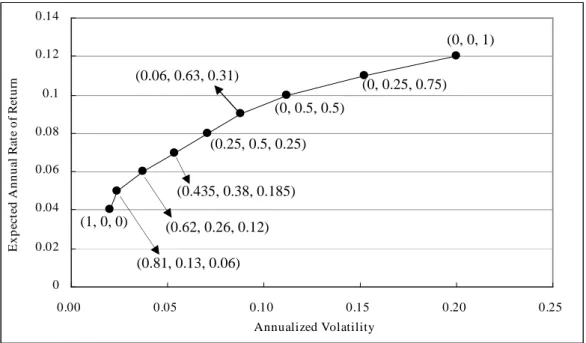
numerical results offered by simulation techniques, a participant chasing the highest

contributions in the portfolio with high expected rate of return and high volatility in

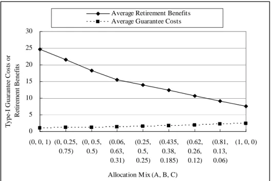
our guarantee designs. After incorporating frequent modification behaviors, averages

and risk measures of guarantee costs may be higher than when the participant always

holds the portfolio with high expected rate of return and volatility. Therefore, when

the pension plan provides rate of return guarantees, the plan provider cannot ignore

the impact of the participant’s frequent modification behaviors.

Keywords: Defined Contribution, Pension Plan, Rate of Return Guarantee,

Martingale Pricing Theory, HJM Model, CIR model, Behavioral Finance,

目

錄

口試委員會審定書...i

謝 辭...ii

中文摘要... iii

Abstract ...iv

The First Essay: Valuation of Interest Rate Guarantees Embedded

in Defined Contribution Pension Plans

...1

1. Introduction...2

2. Structures of Guarantees and Financial Model Settings ...6

3. Valuation of Interest Rate Guarantees... 11

3.1 Type-I Guarantee (Maturity Guarantee) ... 11

3.2 Type-II Guarantee (Multi-Period Guarantee) ...19

4. Numerical Results and Sensitivity Analysis ...23

5. Extension Research under the Setting of Exponentially Decaying Volatility...30

6. Conclusions...39

References...41

Appendix...44

The Second Essay: Impacts of Investment Strategies and

Par

t

i

c

i

pant

s

’

Be

havi

or

s

on

Guar

ant

e

e

Cos

t

s

and

Re

t

i

r

e

me

nt

Benefits in Defined Contribution Pension Plans

...51

1. Introduction...52

2. Structures of Guarantees, Financial Models, and Strategies...58

2.1 Structures of Guarantees ...58

2.2 Interest Rate and Portfolio Price Dynamics...59

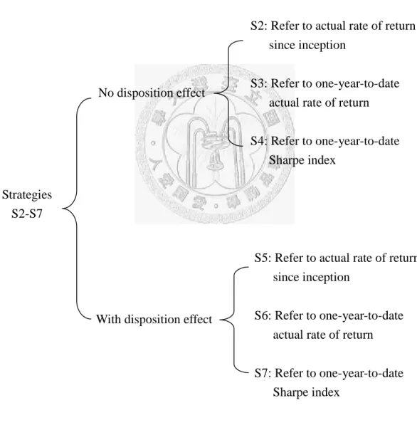
2.3 InvestmentStrategiesand Participants’Behaviors...61

2.4 Actual Rate of Return and Income Replacement Ratio ...65

3. Numerical Results ...66

3.1 Results for S1 (Buy-and-Hold Strategy)...67

3.2 Results for Strategies S2-S7 (with Modification) ...81

4. Conclusions...92

References...94

Valuation of Interest Rate Guarantees Embedded

in Defined Contribution Pension Plans

Abstract

This paper derives the explicit formulae to value minimum rate of return guarantees

embedded in defined contribution pension plans. Different from previous studies, we

analyze the guarantees linked to the -year spot rates. Two types of guarantees are

considered: maturity guarantee and multi-period guarantee. These guarantees have

mixed features of exchange options, path-dependent options and forward start options.

We adopt the one-factor HJM model to describe the evolution of interest rates. The

closed-form formulae are derived by the martingale pricing theory and Margrabe’s

(1978) approach. We also present numerical results and analyze how the values

1. Introduction

Many countries have shifted the pension mechanism from the defined benefit (DB)

plan to the defined contribution (DC) plan. A DB plan usually promises deterministic

benefits to the participant according to some predetermined formulae. Plan providers

bear the risks of poor investment performance. Once the participant stops working in

one organization and skips to another before retirement, the accumulated pension fund

is stopped and cannot be ported with him or her. In contrast, a DC plan offers each

participant one portable individual account. The participant regularly contributes parts

of wages to this account. Retirement benefits are affected by the investment

performance. Disappointing performance will result in uncomfortable retirement life.

To lessen this negative impact of a DC plan, minimum rate of return guarantees may

be embedded in the plan and the costs are covered by guarantee providers, such as

governments or financial organizations.

Among the guarantees commonly seen around the world, some are granted in a

deterministic manner, whereas others are stochastic and linked to rates of return on a

reference portfolio or interest rates. Lindset (2004) names the deterministic type as the

absolute guarantee and the stochastic type as the relative guarantee. In addition,

categorized into two forms, maturity guarantee and multi-period guarantee, according

to when the guarantee is obliged. The maturity guarantee is binding only at expiration

of the pension plan, and the multi-period guarantee specifies a minimum rate of return

binding in each period.

The valuation of maturity guarantees or multi-period guarantees associated with

pension plans or life insurance contracts has been widely studied. The studies mostly

focused on absolute guarantees, including Brennan and Schwartz (1976), Boyle and

Schwartz (1977), Ekern and Persson (1996), Boyle and Hardy (1997), Persson and

Aase (1997), Grosen and Jørgensen (1997, 2000), Miltersen and Persson (1999),

Hansen and Miltersen (2002), and Schrager and Pelsser (2004). Recently, more and

more papers have started to analyze relative guarantees, and the guaranteed rate is

usually measured by the rate of return on the reference portfolio. The valuation

methodology for the relative guarantee is much more complicated than that for the

absolute guarantee because it has to incorporate the rate of return process of the

reference portfolio. Ekern and Persson (1996) deal with the relative guarantees

embedded in unit-linked life insurance contracts. Pennacchi (1999) obtains the values

of relative guarantees provided in DC plans by explicit formulae or by using Monte

(henceforth, HJM) (1992) to deriving closed-form pricing formulae for different

pension contracts embedded with minimum guaranteed rates of return. In all of these

three papers, guaranteed rates are linked to the performance of the reference portfolio

whose price follows the geometric Brownian motion.

Extending prior studies, we consider the relative guarantees linked to the -year spot

rates, which means that the guarantees are interest rate guarantees. This design is

attractive to both guarantee providers and pension participants. Compared with the

rate of return on a reference portfolio traded in the equity market, -year spot rates

are less easily manipulated by individuals and organizations. In addition, the pension

plan has to guarantee the rate of return which can be obtained in the market. If not,

participants would rather put money in the certificates of deposit issued by banks than

join the pension plan.

Our objective is to determine the fair values of both maturity and multi-period interest

rate guarantees. The interest rate guarantees under analysis have several features. First,

the payoff of the pension plan embedded with either of these guarantees is similar to

that of the exchange option. Second, the guaranteed rates are dependent on the path of

retirement. This path-dependent feature is also seen in many exotic options, such as

the Asian option.1 Finally, some of the embedded guarantees are calculated from the specific time in the future. This resembles the forward start option.2 In order to value the interest rate guarantees, the valuation framework has to incorporate two stochastic

processes to characterize the price of the underlying investment portfolio and the

stochastic interest rate. The price of the underlying investment portfolio is assumed to

follow a geometric Brownian motion. The evolution of interest rates is described by

the one-factor HJM model. We adopt the martingale pricing theory and Margrabe’s

(1978) approach to derive the values of both guarantees.

The remaining paper is organized as follows. Section 2 presents the structures of

guarantees and financial model settings. The closed-form formulae for both types of

guarantees are derived in section 3. We provide numerical results for the values of

these guarantees and carry out the sensitivity analysis in section 4. Section 5 extends

the proceeding study by setting different diffusion factor in the HJM model. Section 6

concludes this paper and proposes further research directions.

1 _{According to Hull (2000), the payoff of the Asian option depends on the arithmetic or geometric}

average price of the underlying asset during some period within the lifetime of the option.

2 _{According to Hull (2000), the forward start option is the option that will start in the future. Bouaziz} et al. (1994) and Tsao et al. (2003) discuss the pricing of forward-starting Asian options, where the

price of the underlying asset follows lognormal distribution and the strike price is computed as the arithmetic average of the underlying asset prices over one period in the future. No dynamic of

2. Structures of Guarantees and Financial Model Settings

First we present the basic structure of the pension plan analyzed in this study. During

the accumulation phase, the participant contributes at the first day of each year. The

actual rate of return and the guaranteed rate are calculated at several record dates,

each of which is the last calendar day of each year. The timeline of the pension plan is

shown in Figure 1. One participant starts to work and selects one investment portfolio

at t=0. The investment portfolio is held until retirement. The yearly wages in the first

year are Y . The annual growth rate of wages is k. At the n-th year, the participant’0 s

yearly wages are Y₀(1k)n1. The participant does not retire until time T. During these T years, the percentage of wages contributed by a participant to the individual

account per year is fixed at c. We neglect administrative costs and the case that the

Yearly Wages Y₀ Y₁ …… Y_T2 Y_T1 Y_T

Actual return rate R₁ …… R_T2 R_T1 R_T

Guaranteed R₁ …… R_T2 RT1 RT

return rate

Figure 1. Timeline of the Pension Plan

The amount contributed to the individual account in the first year is Y0c. Assume

that R is the actual rate of return in the t-th year. At the first record date (the lastt

calendar day of the first year), the value of the first contribution becomes

) exp( 1 0 c R

Y  ; at the second record date, it becomes Y0cexp(R1)exp(R2); at time

T, this amount changes to



   T t t R c Y 1

0 exp( ) according to the actual investment

performance. Similarly, the amount contributed in the n-th year changes to

) exp( ) 1 ( 1 0 t T n t n R k c Y  _  

 at time T. Summing up actual payoffs of the

contributions of each year, we have



  _    T n t T n t n R k c Y 1 1

0 (1 ) exp( ), which are the

benefits the participant receives at time T without any guarantee and is named as

“actual benefits.”

Accumulation Phase;

Contribute parts of yearly wages to the individual account in each year

before retirement

Record date 0 1 …… T-2 T-1 T

Retirement date Start to work;

In each year over the life of the plan, the guarantee provider offers a minimum

continuously compounded annual rate of return, which is equal to the -year spot

rate at each record date. Let R(t,t) be the minimum guaranteed rate of return at

time t. Two types of guarantees are considered. If the guarantee is binding only at

expiration of the pension plan, we called it a “type-I guarantee,”which is a maturity

guarantee. If the minimum guaranteed rate of return is binding for each period, we

refer it as a “type-II guarantee,”which is a multi-period guarantee.

Under the type-I guarantee, we express the retirement benefits a participant claims

when retiring at time T as



         _{  }       T n t T n t T n t n T I Y c k Max R t t R 1 1 0 (1 ) exp( (, )), exp( ) ) ( 



           _      _{  }     T n t T n t t T n t T n t n R R t t R Max k c Y 1 1

0 (1 ) exp( ( , )) exp( ),0 exp( ) , (1)

where



         _{  }     T n t T n t T n t n R t t R Max k c Y 1 1

0 (1 ) exp( ( , )) exp( ),0 is the amount the

guarantee provider has to compensate for the type-I guarantee.

Under the type-II guarantee, we express the retirement benefits received at time T as









  _{ }      T n t t T n n

T(II) Y c (1 k) Maxexp(R(t,t )),exp(R )

1 1 0  , (2) and





      _{ }    







    T n t t T n t t T n n R R t t R Max k c

Y (1 ) exp( ( , )),exp( ) exp( )

1

1

0  is the

Equations (1) and (2) reflect that the payoffs of the defined contribution pension plans

embedded with the type-I or type-II guarantees have some interesting features. First,

both payoffs have similar structure to the payoff of the exchange option. Second,

these payoffs depend on the paths of the actual rate of return on the underlying

investment portfolio, R , and the guaranteed rate of return,_t R(t,t). Third, some

of the embedded guarantees are not calculated from the inception of the pension plan

but from the specific time in the future.3

Now we illustrate how to calculate R_t and R(t,t). Under the risk-neutral

measure Q, the price of the investment portfolio per share, S_t , follows the stochastic

process: t t S t t t rS dt S dZ dS   , (3)

where _S  is the constant diffusion factor of the portfolio price, r is the_t

risk-free short rate, and



Z_t :t0



is a standard one-dimensional Q-measure Brownian motion.

3

The payoff structures in this paper are different from those in Lindset (2004). We define the guaranteed rate as the δ-year spot rate at time t. Instead, Lindset (2004) defines the guaranteed rate in any period t as the rate of return on the reference portfolio between time t-1 to t. Furthermore, we plan to calculate the single premium paid at t=0 for the guarantee so we not only take the first contribution into account but also allow that n>1. Lindset (2004) only considers $1 contributed

The actual rate of return on this portfolio R_t is defined as: ) / ln( _1  _{t t} t S S R , t 1,2,...,T. (4)

When the price of the underlying investment portfolio follows the geometric

Brownian motion, R_t is normally distributed.

We apply the HJM framework to deriving short rates and spot rates. According to

Heath et al. (1992), the instantaneous forward rate process under the risk-neutral

measure Q is t f u t f f t u t x dx dt t u dW u t df(, ) ( , ) ( , )  ( , )      

_

, (5)

where ut and



W_t :t0



is a standard one-dimensional Q-measure Brownian motion correlated with Z_t and satisfies dW_tdZ_t dt for all [1,1] .

Therefore, after considering another standard one-dimensional Q-measure Brownian

motion W_t' independent of W , we can rewrite_t dZ_t dW_t  12dW_t'. The diffusion factor, f( ut, ), plays an important role in the HJM model. We first assume

that f( ut, ) is a constant, i.e., f(t,u)f 0, then we can rewrite equation (5)

as t f f u t dt dW u t df(, )(2( ))  . (6)

The HJM model with constant volatility factor can be viewed as the continuous-time

limit of the Ho-Lee (1986) model. By equation (6), the instantaneous forward rate is

t f f W t u t u f u t f           2 ) , 0 ( ) , ( 2 ;

the short rate r is_t

t f f t f t t W r   2  2 2 ) , 0 ( ; (7)

the time-t price of a zero-coupon bond maturing at time t+ is

               f _{f t} W t t t P t P t t P    ( )  2 exp ) , 0 ( ) , 0 ( ) , ( 2 , where _      

_

t du u f t P 0 (0, ) exp ) , 0

( ; and the time-t spot rate for maturity t+ is

          f t f W t t t P t P t t t t P t t R              ln (0, ) ln (0, ) 2 ( ) ) ( ) , ( ln ) , ( 2 t fW t g   1() , (8) where g1(t) ( ) 2 ) , 0 ( ln ) , 0 ( ln 2 _   _{ }   t t t P t P f

. From these expressions, we

know that the guaranteed rate of return R(t,t) is normally distributed.

3. Valuation of Interest Rate Guarantees

3.1 Type-I Guarantee (Maturity Guarantee)

This section derives the value of the type-I guarantee. Define V_T(I) as the terminal



         _{  }     T n t T n t T n t n T I Y c k Max R t t R V 1 1 0 (1 ) exp( (, )) exp( ),0 ) (  . (9)

Also define T(n)(I) as the time-T value of the type-I guarantee for one dollar contributed in the n-th year, nT, i.e.,

      _{ } 





  0 , ) exp( )) , ( exp( ) ( ) ( T n t t T n t n T I Max R t t  R  . Let



  T n t n T R t t A₁( ) exp( ( , )) and



 T n t t n T R

A₂( ) exp( ) , then we have ] 0 , [ ) ( 2( ) ) ( 1 ) ( n T n T n T I Max A A  .

Proposition 1: Given that the time-T value of the type-I guarantee for one dollar

contributed in the n-th year is T(n)(I). The time-0 market value of ( )

) ( I n T  is ) ( ) ( ) ( ₁₀( ) ₁( ) ₂₀( ) ₂( ) ) ( 0 n n n n n d A d A I      , where ) ( 10 n A





                ( 1)( 2) 6 ) , ( exp 2 2 n T T n n n g f , ) ( 20 n A _      

_

n 1f u du 0 (0, ) exp ,  ) ( 1 t g ( ) 2 ) , 0 ( ln ) , 0 ( ln 2 _   _{ }   t t t P t P f , 6 ) , 0 ( ) ( ) , ( 3 2 0 1 2 T du u f t g T n g T f T n t          





 , T T A A d _n n n n n ) ˆ ( 2 / ) ˆ ( ) / ln( ) ( 2 ) ( ) ( 20 ) ( 10 ) ( 1     , d n d1(n) (ˆ(n)) T ) ( 2   , T n) 2 ( ) ˆ ( ) 3 )( 1 ( 2 2 S f S f n T       , and ) (

 denotes the cumulative probability function for a variable followed by a

After considering the contributions in each year and total accumulations, the value of

the type-I guarantee is V₀(I)



 _    T n n n I k c Y 1 ) ( 0 1 0 (1 )  ( ).

Proof: The complete proof is broken into six steps.  Step 1: Changing numeraire.

We follow the approach in Margrabe (1978). Treating the asset with time-T value of

) ( 2

n T

A as numeraire, the time-0 value of one contingent claim whose payoff at

expiration date T is equal to T(n)(I) can be derived by the following equation:          ) ( 2 ) ( ˆ 0 ) ( 20 ) ( 0 ( ) ( ) n T n T n n A I A I   ,

where 0ˆ



denotes the expectation function under ˆmeasure conditional on the

market information up to time 0. This equation comes from the martingale pricing

approach and reflects that the process of _{( )}

2 ) ( ) ( n t n t A I 

is a martingale under ˆmeasure.

Then,            ) ( 2 ) ( 2 ) ( 1 ˆ 0 ) ( 20 ) ( 0 ) 0 , ( ) ( _n T n T n T n n A A A Max A I                       0 , 1 ) ( 2 ) ( 1 ˆ 0 ) ( 20 n T n T n A A Max A . We view _        01, ) ( 2 ) ( 1 n T n T A A

Max as the time-T payoff of one option whose strike price is

unity and the time-T price of the underlying asset is 2( ) ) ( 1 / n T n T A A . 1( ) n T A , 2( ) n T A , and

) ( 2 ) ( 1 / n T n T A

A are all lognormally distributed, so we can apply the formula in Hull (2000)

and obtain that

           ( ) 1 ( ) ) ( _{( ) 1}( ) ₂( ) 20 ) ( 10 ) ( 20 ) ( 0 n n n n n n d d A A A I  ) ( ) ( ₁( ) ₂₀( ) ₂( ) ) ( 10 n n n n d A d A     ,

where A₁₀(n) is the time-0 price of A₁(_Tn) , A₂₀(n) is the time-0 price of A₂(n_T) ,

T T A A d _n n n n n ) ˆ ( 2 / ) ˆ ( ) / ln( ) ( 2 ) ( ) ( 20 ) ( 10 ) ( 1     , d n d1(n) (ˆ(n)) T ) ( 2   , and T n) 2 ( ) ˆ ( is equal

to Var₀Q[ln(A₁(_Tn)/A₂(_Tn))] Var₀Q

 

lnA₁(_Tn) Var₀Q

 

lnA₂(_Tn) 2Cov₀Q



lnA₁(_Tn),lnA₂(_Tn)



. We calculate A₁₀(n) , A₂₀(n) , Var₀Q

 

lnA₁(_Tn) , Var₀Q

 

lnA₂(_Tn) and Cov₀Q



lnA₁(_Tn),lnA₂(n_T)



in the following steps.

 Step 2: Find ( ) 10

n

A , the time-0 price of A₁(_Tn).

Since A₁₀(n) is not necessary observed in the market, we have to calculate the value of

) ( 10

n

A . By the martingale pricing approach, A₁₀(n) is equivalent to ₀Q[A₁(_Tn)B_T1], where

] [

0 

Q

E is the expectation function under the risk-neutral measure Q conditional on the

market information up to time 0, and B_T is the cash account at time T. With risk-free

rate r ,_u B_T is defined as _      

_

T u T B r du B 0

0exp and B =1. Then,0

) ( 10 n A ₀Q[A₁(_Tn)B_T1]       _{  }  



_

 ) exp( )) , ( exp( 0 0 T u T n t Q du r t t R 





                       



_

_

 T T u f f T n t t f Q du W T du u f W t g 0 0 3 2 1 0 6 ) , 0 ( ) ( exp    (Let 6 ) , 0 ( ) ( ) , ( 3 2 0 1 2 T u d u f t g T n g T f T n t          





 )             _{ }  



_

 T n t T u f t f Q du W W T n g 0 2 0 exp ( , )               _  



_

 T n t T u f t f Q du W W Var T n g 0 0 2 2 1 ) , ( exp  





                ( 1)( 2) 6 ) , ( exp 2 2 nT T n n n g f .

The derivation of the last equation can be read in Appendix (A).

 Step 3: Find ( ) 20

n

A , the time-0 price of A₂(n_T).

Also by the martingale pricing approach, we have A₂₀(n) ₀Q[A₂(n_T)B_T1]. Then,

] ) exp( [ ] [ ₂( ) 1 ₀ 1 0 ) ( 20    _{ }  



T T n t t Q T n T Q n B R B A A            1 1 0 T n T Q B S S                          _{  }        _{ }   







  T u n S S n u T S S T u Q du r Z n du r S Z T du r S 0 1 2 1 0 0 2 0 0 0 exp ) 1 ( 2 1 exp 2 1 exp                _{     }  

_

 ( 1) ( _) 2 1 exp 1 2 ₁ 0 0 S S T n n u Q Z Z n T du r  

              

_



_

1 0 3 2 1 0 0 6 ) 1 ( ) , 0 ( exp n f _f n _u Q du W n du u f            



 T n u S S T n ₁dZ 2 ) 1 ( 2 1_{ } (Let ( 1) 2 1 6 ) 1 ( ) , 0 ( ) , ( 2 3 2 1 0       

_

f u du n T n T n h n f _S )             _{  }  

_

_

  T n u S n u f Q dZ dW u n T n h 1 1 0 0 exp ( , )  ( 1 )             _{  }   





  T n u S n u f Q dZ dW u n Var T n h 1 1 0 0 ( 1 ) 2 1 ) , ( exp                      _{ }   





  T n u S Q n u f Q dZ Var dW u n Var T n h 1 0 1 0 0 2 1 ) 1 ( 2 1 ) , ( exp         _{    } 





  T n S n f n u du du T n h 1 2 1 0 2 2 2 1 ) 1 ( 2 1 ) , ( exp         _{      }  ( 1) 2 1 ) 1 ( 6 1 ) , ( exp h n T 2_f n 3 _S2 T n       

_

n 1 f u du 0 (0, ) exp .  Step 4: Find

 

( ) 1 0 ln n T Q A Var .

 

( ) 1 0 ln n T Q A Var       _ 



 T n t Q t t R Var₀ ln exp( ( , ))       _ 



 T n t Q t t R Var₀ (, )       



 T n t t f Q W Var₀                  6 ) 1 2 2 )( 1 )( ( ) 1 ( 2 2 T n T n T n n T n f  .

 Step 5: Find

 

( ) 2 0 ln n T Q A Var .

 

( ) 2 0 ln n T Q A Var )] / [ln( ₁ 0   Q _{T n} S S Var                                  





) ) 1 ( 2 1 exp( ) 2 1 exp( ln 1 2 1 0 0 2 0 0 0 n S S n u T S S T u Q Z n du r S Z T du r S Var        

_

 T n u f Q du W Var 1 0  



_ _ T n u S ₁dZ                _{  }  

_

_

_

  T n u Q S T n u u Q f Var T u dW n u dW Var0 ₁dZ 2 0 1 0 0 2 ) 1 ( ) (         _{  }   

_

_

_

  T n u T n u u Q S f Cov ₀ T u dW n u dW ₁dW 1 0 0 ( ) ( 1 ) , 2         _           _  

_

_

1 0 0 0 0 2 ) 1 ( ) ( Q n _u T u Q f Var T u dW Var n u dW           _{ } 

_

T

_

n u u Q dW u n dW u T Cov 0 1 0 0 ( ) , ( 1 ) 2        

_

 T n u Q S Var0 ₁dZ 2  _      _  

_

_

  T n u T n u Q S f Cov0 ₁(T u)dW , ₁dW 2



_

_



_





          1 0 1 0 2 0 2 2 ) 1 )( ( 2 ) 1 ( ) ( n n T f T u du n u du T u n u du 



   T n S du 1 2 

_

    T n S f T u du 1( ) 2 ) 1 ( 3 ) 1 3 ( ) 1 ( 3 ) 1 ( 3 2 2 3 3 2           _  _     _f T n n T n _S T n 2 ) 1 (   _f_S T n .

 Step 6: Find



( )



2 ) ( 1 0 ln ,ln n T n T Q A A Cov .



( )



2 ) ( 1 0 ln ,ln n T n T Q A A Cov       _  _ 



exp( ( , )),ln( / ) ln ₁ 0 T n T n t Q S S t t R Cov     



 T n t t f Q W Cov₀  ,



 T n u f ₁W du  _   



 T n u S ₁dZ     



 T n t t f Q W Cov₀  ,



 T n u f ₁W du  _   



 T n u S ₁dW         

 

  T n t T n u t Q f Cov0 W ₁W du 2 ,  + _      



_

  T n u T n t t Q S f Cov0 W , ₁dW  .

In the last equation,

     

 

_  T n t T n u t Q du W W Cov 1 0 ,       _{  } 



_

_

_

  T n t n u T u t u Q dW u n dW u T dW Cov 1 0 0 0 0 , ( ) ( 1 )



_{ } _





 __ _





  ___ T n t n u t u Q T u t u Q dW u n dW Cov dW u T dW Cov 1 0 0 0 0 0 0 , ( ) , ( 1 )



_ _



 



  _ T n t n t du u n du u T 1 0 0( ) ( 1 )



      _{ }  T n t n t Tt 2 ) 1 ( 2 2 2 12 ) 1 2 )( 1 ( ) 1 2 )( 1 ( 2 ] ) 1 ( ) ( )[ 1 ( 2            T n T T n n T T T n n n , and      





_  T n u T n t t Q dW W Cov 1 0 ,       



_

  T n u T n t t u Q dW dW Cov 1 0 0 ,



_





      T n t T n u t u Q dW dW Cov 1 0 0 ,



_





      T n t t n u t u Q dW dW Cov 1 0 0 ,



_  T n t t ndu1



   T n t n t 1) ( 2 ) 2 )( 1 (     T n T n .

Then the expression of Cov₀Q



lnA₁(_Tn),lnA₂(n_T)



is written as



( )



2 ) ( 1 0 ln ,ln n T n T Q A A Cov            _        12 ) 1 2 )( 1 ( ) 1 2 )( 1 ( 2 ] ) 1 ( ) ( )[ 1 ( 2 2 T n T T n n T T T n n n f  2 ) 2 )( 1 (      _f_S T n T n . □

3.2 Type-II Guarantee (Multi-Period Guarantee)

This section derives the value of the type-II guarantee. Define V_T(II) as the terminal

market value of the type-II guarantee, which is





      _{ }     







    T n t t T n t t T n n T II Y c k Max R t t R R

V ( ) (1 ) exp( (, )),exp( ) exp( )

1

1

0  . (10)

Also define T(n)(II) as the time-T value of the type-II guarantee for one dollar contributed in the n-th year, nT . T(n)(II) is expressed as:





_



     T n t t T n t t n

T (II) Maxexp(R(t,t )),exp(R ) exp(R )

) (   . Let







  T n t t n T Max R t t R

A₃( ) exp( ( , )),exp( ) and



 T n t t n T R

A₂( ) exp( ), then we have

) ( 2 ) ( 3 ) ( ) ( _Tn n_T n T II A A  .

Proposition 2: Given that the time-T value of the type-II guarantee for one dollar

contributed in the n-th year is T(n)(II). The time-0 market value of ( )

) ( II n T  is ) ( 20 ) ( 30 ) ( 0 ( ) n n n A A II    , where                                 



 T n t t t f n d d t g A ( ) ( ) 1 6 ) ( exp 3 4 2 3 ) ( 30        



1 0 (0, ) exp n f u du , ) ( 20 n A _      

_

n 1f u du 0 (0, ) exp , t d₃ t t t g t t f         ~ 2 ~ 6 ) ( 2 2 3 , t d d4t  3t ~t  ,  ) ( 1 t g ( ) 2 ) , 0 ( ln ) , 0 ( ln 2 _   _{ }   t t t P t P f , ) ( ) 1 3 3 ( 6 ) , 0 ( ) ( 2 ₁ 2 1 3 t f u du t t g t g t f t      

_

  , S f S f t t       2  2 2 3 ~ _{, and} ) (

 denotes the cumulative probability function for a variable followed by a

standardized normal distribution.

After considering the contributions in each year and total accumulations, the value of

the type-II guarantee is



 _    T n n n II k c Y II V 1 ) ( 0 1 0 0( ) (1 )  ( ). Proof:

The time-0 value of A₂(_Tn), or A₂₀(n), has been derived. We need only to calculate the time-0 value of A₃(_Tn), or A₃₀(n). By the martingale pricing approach,

] [ ₃( ) 1 0 ) ( 30    n _T T Q n B A A





      _{  }  



_

 ) exp( ) exp( )), , ( exp( 0 0 T u T n t t Q du r R t t R Max 





      _{  }  



_

  ) exp( / )), , ( exp( 0 1 0 T u T n t t t Q du r S S t t R Max 





               _{ }   



_

_

   T n t t t u S S t t u t f Q dZ du r W t g Max 1 2 1 1 0 2 1 exp , ) ( exp          



_

_

   1 0 1 ) exp( ) exp( n _u T n t t t rudu r du               _{ }      _{  }  



_

_

   T n t t t u S S t f t t u Q dZ W t g du r Max 1 2 1 1 0 2 1 exp , ) ( exp   





   1 0 ) exp( n rudu .

According to Appendix (B), the terms f t t t rudug t W 



 1( ) 1 can be simplified to



   t t u f u t dW t g 1 3( )  ( 1) , where (3 3 1) ( ) 6 ) , 0 ( ) ( 2 ₁ 2 1 3 t f u du t t g t g t f t      

_

  .

Therefore, A₃₀(n) can be further reduced so that

              _{ }       _{ }  



_

_

   T n t t t u S S t t u f Q n dZ dW t u t g Max A 1 2 1 3 0 ) ( 30 2 1 exp , ) 1 ( ) ( exp   





   1 0 ) exp( n rudu



_

_

                   _{ }       _{ }  T n t t t u S S t t u f Q dZ dW t u t g Max 1 2 1 3 0 2 1 exp , ) 1 ( ) ( exp            

_

1 0 0 exp( ) n u Q du r .

The last equation comes from the property of independent increment of Brownian

motion. It is simple to prove that _

      

_

1 0 0 exp( ) n u Q du r is equal to

     

_

1 0 (0, )

exp n f u du . To calculate the first expectation value in the last equation, let

      _{ } 

_

 t t u f t g t u t dW X 1 3 1 exp ( )  ( 1) and      _{ } 



 t t u S S t dZ X 1 2 2 2 1 exp   , then                  _{ }       _{ } 

_

_

  t t u S S t t u f Q dZ dW t u t g Max 1 2 1 3 0 2 1 exp , ) 1 ( ) ( exp    )] , ( [ _{1 2} 0 t t Q X X Max   ) ( ] ) 0 , ( [ _{1 2} 1 _{0 2} 0 t Q t t t t t Q X B B X B X Max       .

Both X_1tB_t and X_2tB_t are lognormally distributed. Consider one contingent claim whose payoff at time t is Max(X_1tB_t X_2tB_t,0), which can be viewed as the payoff of an exchange option exercised at time t. Then ₀Q[Max(X_1tB_t X_2tB_t,0)B_t1] is the time-0 value of this contingent claim under the risk-neutral measure Q. Given that

there exists no arbitrage opportunity, the time-0 value of Max(X_1tB_t X_2tB_t ,0)

should be unique no matter what asset is applied to be the numeraire in valuation.

Instead of directly computing ₀Q[Max(X_1tB_t X_2tB_t ,0)B_t1], we again follow Margrabe’s (1978) pricing method so that the time-0 value of this claim is

) ( ) ( ) ( ) ( _{1 3 0 2 4} 0 t t Q t t Q d X d X   

 , where Q₀(X_1t)₀Q(X_1tB_t B_t1) is the time-0 price of X_1tB_t , ₀Q(X_2t)Q₀(X_2tB_t B_t1) is the time-0 price of X_2tB_t ,

t t X X d t t t Q t Q t         ~ 2 / ~ )] ( / ) ( ln[ _{0 1 0 2} 2 3 , d t d t tt ~ 3 4 , and t t 2 ~  is defined as                              t t Q t t t t Q X X Var B X B X Var 2 1 0 2 1 0 ln ln .

It is easy to show that _          6 ) ( exp ) ( 2 3 1 0 f t Q t g X  and 0 ( 2t)1 Q X . From

Appendix (C), we know that 0

3 ~ 2 2 2    S f S f t t     . Consequently, we have this proposition. □

4. Numerical Results and Sensitivity Analysis

This section provides the numerical results for V₀ (I), V₀ (II), and shows how these values vary with some key parameter estimates, while keeping all the other parameter

estimates unchanged. To justify the values derived by Proposition 1 and Proposition 2,

we also list the values obtained by Monte Carlo simulation. The procedure of

simulation is described as follows.

Step 1: Given the parameters estimates, simulate weekly prices of the investment

portfolio by equation (3). We consider the discretization error here. The

details about this are reported in Appendix (D).

Step 2: At the last day of each year, calculate the actual rate of return by equation (4)

and the guaranteed rate by equation (8). Record the actual rate of return and

the guaranteed rate.

Step 3: At time T, calculate V_T(I) by equation (9) and V_T(II) by equation (10).

) ( ˆ ) ( exp ₀ 0 r du VT I V I T u    



_

, and the present value of V_T(II) for this path is computed as exp ( ) ˆ₀( ) 0 r du VT II V II T u    



_

. From this step we know that the price derived by simulation is under the risk-neutral measure Q. We

consider the discretization error when deriving      

_

T udu r 0

exp . The details

about this are described in Appendix (D).

Step 4: Repeat steps 1-3 for 50,000 paths. Calculate the arithmetic average of Vˆ0(I) (or Vˆ0(II)) over the 50,000 paths and then derive the fair value of the type-I (or type-II) guarantee. The results are reported in column (B) of Table 1.

The basic parameter estimates are as follows:4

30  T , Y₀ 1, k 0.03, c0.06, 1 0  S , 2, S 0.1, f 0.01, 0.2.

Furthermore, we also assume that the initial term structure is flat and fixed at 3%, so

t

e t

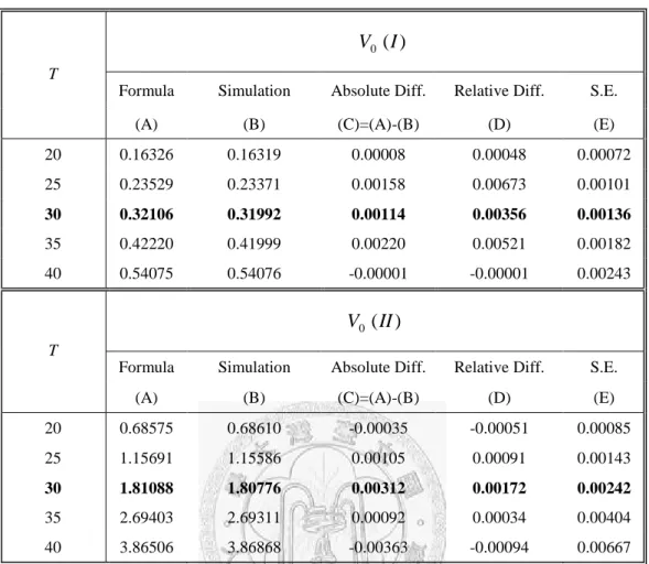
P(0, ) 0.03 . Under these settings, V₀ (I) is 0.32106 and V₀ (II) is 1.81088. Numerical results are listed in Table 1 and Figures 2-3. We have some findings.

(i) Table 1 shows that the difference between the value derived by the explicit

formula and the value derived by simulation is tiny. This demonstrates that the

formulae provide one accurate way to value the interest rate guarantees. The term

4 _{From Proposition 1 and Proposition 2, we know that the values of both guarantees are irrelevant to}

the initial price of the investment portfolio, S0. Therefore, we do not need to set up S0when valuing

both guarantees by these two propositions. However, in order to produce the weekly price of the investment portfolio when carrying out simulation, the setting of S0is required.

of the pension plan is usually very long. Deriving the value by simulation is very

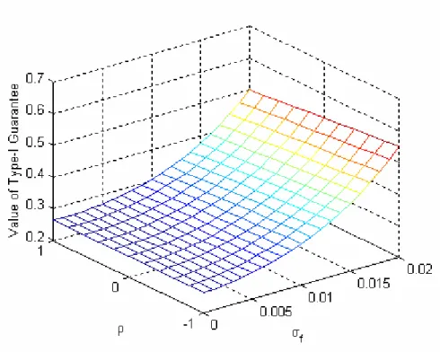
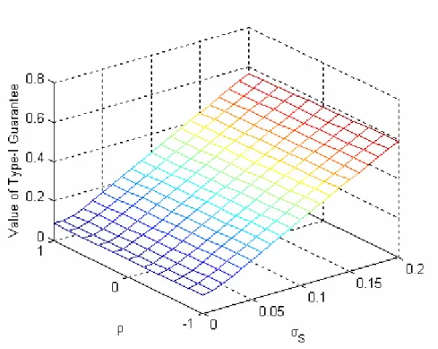
time-consuming.5 It is an efficient way to price these guarantees by our formulae. (ii) Figures 2 and 3 reveal that all values decrease as the correlation estimate becomes

higher, except for the cases that f 0 or S 0. This is due to the fact that

2 ) (

) ˆ

(n in Proposition 1 and  in Proposition 2 are both decreasing functions~_t2 of  when _f 0 and _S 0. If _f 0 or _S 0, (ˆ(n))2 and  are~_t2 irrelevant to  therefore the values do not change with .

(iii)High forward rate volatility ( ) or volatility of the investment portfolio pricef

( ) has two effects. AsS  orf  increases, the probability that the actual rateS

of return on the investment portfolio significantly falls below the guaranteed rate

of return increases as well. However, the first derivative of (ˆ(n))2 and ~_t2 with respect to  (orf  ) may be negative, especially in the case that  isS

close to +1 and  (orf  ) is very small. These effects work together so thatS

higher  (or_f  ) does not necessary cause higher_S V₀ (I) and V₀ (II), depending on the estimates of  and  (orf  ) , as shown in Figures 2 andS

3.

(iv)The type-I guarantee is not more expensive than the type-II guarantee. For the

mitigated by smaller guaranteed rates appeared in other years. For the type-II

guarantee, such mitigation does not work and being multiplied by subsequent

maximum terms enhances the effects of large guaranteed rates. Thus, the value of

Table 1. Fair Values of the Type-I and Type-II Guarantees: f(t,u)f 0 )

(

0 I V

Formula Simulation Absolute Diff. Relative Diff. S.E.

T

(A) (B) (C)=(A)-(B) (D) (E) 20 0.16326 0.16319 0.00008 0.00048 0.00072 25 0.23529 0.23371 0.00158 0.00673 0.00101 30 0.32106 0.31992 0.00114 0.00356 0.00136 35 0.42220 0.41999 0.00220 0.00521 0.00182 40 0.54075 0.54076 -0.00001 -0.00001 0.00243 ) ( 0 II V

Formula Simulation Absolute Diff. Relative Diff. S.E.

T

(A) (B) (C)=(A)-(B) (D) (E) 20 0.68575 0.68610 -0.00035 -0.00051 0.00085 25 1.15691 1.15586 0.00105 0.00091 0.00143

30 1.81088 1.80776 0.00312 0.00172 0.00242

35 2.69403 2.69311 0.00092 0.00034 0.00404 40 3.86506 3.86868 -0.00363 -0.00094 0.00667 Notes: Column (A) lists the values derived by the formulae in the propositions. Column (B) lists the values derived by simulation based on 50,000 paths. Column (C) describes the absolute difference between (A) and (B), and column (D) describes the relative difference, which is equal to the value in (C) divided by the value in (A). Column (E) reports the standard error of the simulation estimates.

Figure 2-I. Value of Type-I Guarantee, Given Different  and f

Figure 3-I. Value of Type-I Guarantee, Given Different  and S

5. Extension Research under the Setting of Exponentially Decaying

Volatility

The preceding two propositions are derived by assuming that the volatility term in the

HJM model is constant. Flesaker (1993) uses GMM test to demonstrate that the

constant-volatility HJM model is rejected in the daily data for Eurodollar futures

options. However, from Amin and Morton (1994) we know that the constant-volatility

model is preferable to other one-parameter and two-parameter models since its

parameter estimates are more stable. Kuo and Paxson (2006) find that among the

simple one-factor HJM models, the EXP-based model produces lower fitting errors

than the constant-volatility model, but the latter outperforms the former in detecting

mispriced options. Hence, it is better to consider two forms of volatility in our

research. This section focuses on pricing the type-I guarantee under the assumption

that the volatility term in the HJM model is described by an exponentially decaying

structure, i.e., _f(t,u)e(ut) 0 , where ut , 0 and 0 . By definition and simple calculation, we obtain that

t t u u t t x t u dW e dt dx e e u t df( , ) 2 ( ) ( )   ( )      _ 



 _ 





t t u t u t u dW e dt e e ( ) ( ) ( ) 2 1       _             _    ,



    _            t v v u t u t u dW e e e e e u f u t f 0 ) ( 2 2 2 2 2 ) 1 ( ) 1 ( ) , 0 ( ) , (      _   ,