應用DANP建立集體決策的標準作業程序：以某半導體封裝測試廠產能擴充為例

全文

(1)!. Creating an SOP incorporating the DANP methodology into group decision making: The case of capacity expansion in a semiconductor OSAT firm DANP. Advisor: Dr. Cheng, Yu-Jen Student: Hsiang, Tai-Jui. O.

(2) Apply DANP to create a SOP in group decision making: The case of capacity Expansion in a semiconductor OSAT firm.

(3) Acknowledgements This thesis has been developed with the support of many people. I would like to first thank my advisor, Dr. Cheng Yu-Jen, for the patience and time put forward into guiding me until the very end. Next, I would also like to thank Elaine Huang for helping me throughout various procedures due to my limited Chinese comprehension. Also, a special thanks to Dr. Chang-Ming Shih for his advising and support throughout my course at National Kaohsiung University. Last but not least, a big thanks to my parents, friends, and colleagues for the massive encouragements throughout. ! ! ! ! ! !. !. i!.

(4) !. DANP. :. (DEMATEL) DANP. DANP. (DANP). !. ii!. (ANP).

(5) Creating an SOP incorporating the DANP methodology into group decision making: The case of capacity expansion in a semiconductor OSAT firm Advisor: Dr. Cheng, Yu-Jen Institute of Business and Management National University of Kaohsiung Student: Hsiang, Tai-Jui Institute of Electrical Engineering National University of Kaohsiung. Abstract This research uses a conceptual hybrid of decision-making trial-and-evaluation laboratory (DEMATEL) in conjunction with the analytic network process (ANP), we effectively eliminate various groupthink biases that parasitically drain resources from corporations, burying itself within plain sight but rarely recognized nor eradicated. Although several literary experts have proposed methods to protect the sanctity and values of optimal decision-making, many have fallen short on several fronts. The SOP created incorporates the DANP methodology in a systematic fashion to decrypt the interrelationships and make sense of varying influences each factor exerts or absorbs from each other. The SOP guides any person who wish for the same decision making refinement in their study. As an example, an additional case study follows in helping to bridge the gap between theoretical methodology and real-life applications to solve a complex problem. Keywords: Standard Operational Procedure (SOP), Groupthink, Multiple Criteria Decision Making (MCDM), DANP (DEMATEAL-based ANP).. !. iii!.

(6) Contents Chapter 1 Introduction ................................................................................................. 1 1.1 Research background and motivation ............................................................... 1 1.2 Research purpose ............................................................................................... 4 1.3 Research contributions ...................................................................................... 6 1.4 Thesis structure .................................................................................................. 6 Chapter 2 Literature Review ....................................................................................... 7 2.1 Groupthink ......................................................................................................... 7 2.2. Bounded rationality .......................................................................................... 9 2.3 Escalating commitment ................................................................................... 10 Chapter 3 Research Methodology ............................................................................. 13 3.1 MCDM ............................................................................................................ 13 3.1.1 DEMATEL ................................................................................................... 14 3.1.2 ANP .............................................................................................................. 14 3.1.3 DANP ........................................................................................................... 15 3.2 Research procedure ......................................................................................... 15 3.2.1 Application of DEMATEL for network relationship ................................... 15 3.2.2 Weight measurements by integrating DEMATEL and ANP ....................... 17 Chapter 4 SOP ........................................................................................................... 20 Chapter 5 A Case Study ............................................................................................ 23 5.1 Measuring relationships among categories ..................................................... 24 5.1.1 The ranking of ("# + %# )' and ("#' − %) ) ................................................... 25 5.1.2 The causal diagram ....................................................................................... 26 5.1.3 The strategy map .......................................................................................... 26 5.2 Weight measuring among factors .................................................................... 27 5.2.1 The Ranking of the factors ........................................................................... 31 Chapter 6 Ending Remarks ........................................................................................ 34 6.1 Conclusion ....................................................................................................... 34 6.2 Discussion........................................................................................................ 34 References ................................................................................................................. 36 Appendix ................................................................................................................... 38. !. iv!.

(7) List of Figures Fig. 1.1 Dilbert Comic Strip ........................................................................................ 2 Fig. 1.2 Illustration of decision making process.......................................................... 4 Fig. 5.1 Causal diagram of total relationship ............................................................ 28 Fig. 5.2 A strategy map of the four categories for capacity expansion ..................... 29. List of Tables Table 1.1 Symptoms of groupthink ............................................................................. 3 Table 3.1 Pair-wise comparisons questionnaire ........................................................ 16 Table 5.1 Definition of key factors............................................................................ 22 Table 5.2 The Initial direct influence matrix A of the four categories ...................... 23 Table 5.3 The normalized direct Influence Matrix X of the four categories ............ 24 Table 5.4 The total influence matrix T of the four perspectives ............................... 26 Table 5.5 The gives and received influences of the four perspectives ...................... 26 Table 5.6 The initial direct influence matrix A of the 16 selected factors ................ 28 Table 5.7 The normalized direct influence matrix X of the 16 selected factors ....... 28 Table 5.8 The total influence matrix T of the 16 selected factors ............................. 29 Table 5.9 The un-weighted super matrix of the 16 selected factors .......................... 29 Table 5.10 The weighted super matrix of the 16 selected factors ............................. 30 Table 5.11 The limiting super matrix of the 16 selected factors ............................... 30 Table 5.12 Weights and ranking ................................................................................ 32 Table 5.13 Points given to each factor in each alternate location ............................. 32 Table 5.14 Summary of each factor weighed with priority ratio .............................. 33. !. v!.

(8) Chapter 1 Introduction 1.1 Research Background and Motivation An often-overlooked statistic buried in everyday life is the average count of decisions one makes per day. A study done by the Cornell University concluded that while subjects constantly under-estimated an average of fifteen food decisions alone, the actual average was actually two hundred and twenty-one. We can infer, and can also assume from this study that the average person makes far more in total on a daily basis (Lang, 2006). Each stacking set of decisions made on daily, weekly, monthly, or even yearly basis incrementally contributes toward a specific result, and each decision path determines the qualitative value of the attained result. Thus, it deems crucial that decisions must execute an effective leap towards the intended path. Much too often, nevertheless, various obstacles hinder progress, only to create more strain as the deadline draws near. Even more detrimental, however, is when poor decisions are made carelessly due to fragmented knowledge or incompetency among contributing members. Moreover, biases inevitably manifest within group members, either ready to be voice against members of an opposing interest, or to simply gain a feeling of contribution. More often than not, members of different job functions tend to seek decisions read out in their favor. In doing so, the more opinionated and/or rhetoric orators possess a large advantage in swaying the votes to their side, especially when many group members are indifferent towards the outcome. Unequal voices pose a significant drawback from a well-balanced and unbiased decision. Consequently, the quality of the project further deviates from its intended trajectory along each of these points. Paralleled by Janis (1972), a widely recognized social psychologist, she coined the word “groupthink” and defined it as “occurs when a group makes faulty !. 1!.

(9) decisions because group pressures lead to a deterioration of “mental efficiency, reality testing, and moral judgment” (p.9). Furthermore, she lists 8 symptoms of groupthink, listed as follows (Table 1): Table 1.1: Symptoms of Groupthink 1) Illusion of invulnerability –Creates excessive optimism that encourages taking extreme risks. 2) Collective rationalization – Members discount warnings and do not reconsider their assumptions. 3) Belief in inherent morality – Members believe in the rightness of their cause and therefore ignore the ethical or moral consequences of their decisions. 4) Stereotyped views of out-groups – Negative views of “enemy” make effective responses to conflict seem unnecessary. 5) Direct pressure on dissenters – Members are under pressure not to express arguments against any of the group’s views. 6) Self-censorship – Doubts and deviations from the perceived group consensus are not expressed. 7) Illusion of unanimity – The majority view and judgments are assumed to be unanimous. 8) Self-appointed ‘mindguards’ – Members protect the group and the leader from information that is problematic or contradictory to the group’s cohesiveness, view, and/or decisions.. Fig. 1.1: Dilbert comic strip Source: <http://www.usmansheikh.com/time-management/group-participation>. !. 2!.

(10) Janis outlined the symptoms prevalent in all companies, so prevalent that Scott Adams, illustrator of the famous comic strips, ‘Dilbert’, felt obligated to comically satire the issue. In his three-window illustration (shown in Fig. 1), a seemingly unlikely character assumes the role of facilitator, 1 and throughout the meeting praises himself for being the only valuable team member, claiming brilliance and worthiness of honor, all the while describing his surrounding members as ‘dolts’.2 In the comic above, we pick up on the exaggerated irony that among the group, the unseemly character of smallest stature and also a species of minority, in a delusional mindset self-basks in praise but insults toward his surrounding group members. The comic’s intention, needless for further interpretation, is to poke fun at a reoccurring problem in a typical groupthink setting. The illustrator brilliantly taps any reader’s hierarchical memory evoking a recent relativity to such a scenario. Past data-logs and internal reports are among the greatest dependencies in good decision making. They help teams learn from past mistakes and also help identify trends of predictive value in which a confident decision can be based upon. Unfortunately, all companies face new challenges when data is not an available resource. Making a big decision without past data and/or experience will inevitably create more room for biases to manifest even more. Meeting rooms, assumingly, are most often the typical settings for this type of poor decision-making.. 1. In a meeting setting, the facilitator plays the host, ensuring topics and time are in accordance with the agenda 2 Definition of Dolt, defined by the Merriam Webster dictionary: “A stupid person” <http://www.merriam-webster.com/dictionary/dolt>. !. 3!.

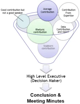
(11) Fig. 1.2: An illustration of decision making process. For a semiconductor OSAT firm in Taiwan, these meeting habits are among the norm. In the typical meeting, the highest-level executive in the group makes the final decision based on the reports presented during the meeting. A key resource used here is the executive’s expertise, along with the past experiences and accumulated knowledge that will help with the decision. Combined with the group consensus, a sensible decision can be made (as shown in fig. 2). However, the disadvantage arises when facing a new issue. Without an objective data source such as past case studies to reference from, a confident decision will unlikely result. This then, poses a problem for the executive, whose next decision will greatly influence the success or failure of the company.. 1.2 Research Purpose In a fast competitively fast evolving technological era, increasingly important is the need to avoid as many potential setbacks as possible—that is, to make minimal mistakes or drop out of the race. Each company, however successful, is at !. 4!.

(12) their level of success due to its accumulated decision consequences, good or bad, that could be traced back to its own founding into the industry. Several methods have been proposed from multiple perspectives to overcome this issue. Although the phrase “no silver/magic bullet” is found true dealing with most complex decisions,3 we can certainly make a refining attempt to streamline the decision making process, such by removing irrelevant noise and clutter from the equation. This paper aims at providing an SOP towards making that confident, unbiased, fully thought-out decision. The decision, made on the basis of a systematic methodology, would be far more reliable than most status quo standards of meetings conducted in companies. For a growing manufacturing company, it is inevitable that capacity expansions must occur in order to satisfy a growing customer base. Mieghem (2003) defines capacity as “a measure of processing abilities and limitations that stem from the scarcity of various processing resources and is represented as a vector of stocks of various processing resources”. In the previously mentioned OSAT firm, its need for expansion is realized when customers/sales’ forecast show more demand than their manufacturing lines can deliver. Before expending capital to expand capacity, the semiconductor OSAT firm needs to take into account all risk factors involved. Five main categories of risk will be discussed, and are as follows: location, finance, environmental regulations, etc. We assume that future uncertainties are driven by fluctuations in the company’s downstream demand. As a result, demand forecasts given to the OSAT company may not always serve as a reliable basis for capacity preparation. As presumed earlier, a company who wants to lead in its industry must make wise and thoroughly unbiased decisions. Therefore, this paper will explore past research on capacity. 3. A complex decision refers mostly to a decision to be made with no simple nor single-factored solution.. !. 5!.

(13) expansion, and different perspectives on how to make the right decisions in such a situation.. 1.3 Research Contribution This paper explores decision making in depth, highlighting various negative influences that lead towards bad decision making. The following section will cover several past papers, including examples of attempts posited to solve these problems. The focal aim of this research is to provide a clear and useful procedure in form of an SOP to overcome symptoms of groupthink and arrive at an optimized solution. Adhering to the SOP will lead the researcher along each step from behind-the-scenes work, and applying the DANP methodology to form a clear data-summary for an optimal decision. A following case study will also serve as an example of how a semiconductor OSAT firm reached its optima solution through application of the SOP.. 1.4 Thesis Structure The following sections will cover several past papers on groupthink and elements that make up its phenomena such as bounded rationality and escalating commitment. Next in chapter 3, the methodology section will introduce the DANP4 method, a hybrid of DEMATEL and ANP. Chapter 4 will provide a walkthrough of a specific SOP to guide the researcher through each step to arrive at an optimal solution. Chapter 5 includes a case study in which we apply the methodology onto a real case adhering to the steps of the SOP. Lastly, in chapter 6, conclusions will be drawn to make a final emphasis on the focal points and the purpose of this research paper.. 4. !. DEMATEL-Based ANP 6!.

(14) Chapter 2 Literature Review A perfect decision involves taking all factors involved and impartially weighing each factor to arrive at an optimal conclusion. However, the process often involves biases within decision makers, whether stemming from pride, arrogance, or just simply lacking confidence. We will introduce some concepts that involve the fore-mentioned traits, and reveal several past literatures on the topic.. 2.1 Groupthink Janis, ten years later after coining the familiar term of Groupthink, further described it in her own words as “a mode of thinking that people engage in when they are deeply involved in a cohesive in-group, when the members’ strivings for unanimity override their motivation to realistically appraise alternative courses of action” (Janis, 1982) This further modification of her description is a collection of common elements present in her earlier listed symptoms of groupthink. They all possess a perceivable tendency for group members to form and polarize towards a consensus in an illusion that the group conformity is more likely to have a more rational, correct decision that is likely to succeed against an opposing challenge from people who they perceived as less reasonable, less likely to succeed, and heading towards the wrong direction. Therefore, in a setting such as this, the group members are concurrence seeking to what they think is the group consensus. A great and growing number of studies and scholarly articles have fixated on Janis’ groupthink theory since its publication. Case studies were cited which dealt with a range of historical settings and situations that fit the profile (Hart, 1991). Experimental studies and well-tested variables were also used to demonstrate the validity and to drain out the ambiguity that gives possible skepticism in arguments for confounding variables. !. 7!.

(15) Von Bergen & Kirk (1978) in their journal entry compares the pros and cons of group decisions versus individual decisions. The biggest benefit is the added value of each member’s collective productivity. A drawback of deciding in a group is the fear of rejection toward one’s idea. A less obvious but relevant factor is the tendency for the group to congregate uniformly towards a decision. Noelle-Neumann (1974), in his paper “spiral of silence”, agrees with the common attitude towards groupthink. He says that in a large group, some group members will rather keep their silence in fear of rejection. A social identity research points to a strong correlation between members’ identification with groups and conformity with collective norms (Terry & Hog, 1996). This view is undoubtedly a negative perspective on groupthink, but not shared by all. The alternative view argues that groupthink is actually not as pessimistic. Packer’s normative conflict model argues that certain groupthink elements actually result in a better decision. The louder, more voiced opinions often come from more engaged and attentive group members. They are also often more receptive to social costs, and less discouraged by rejection or other forms of criticism. The willingness to challenge group norms, on its own, solves various groupthink elements. Group composition is related to the upper echelon perspective of organizations. Hambrick & Mason (1984) wrote, “The theory states that organizational outcomes can be partially predicted from managerial backgrounds”. The perspective suggests that observable traits of decision makers such as age, education, and group characteristics have an impact on strategic choices, and in turn on performances of firms. Studies have found relationships between group compositions and performances (Goll, Sambharya & Tucci, 2001). Other studies have explored the relationship between heterogeneity in groups (Murray, 1989; Hambrick, Cho & Chen, 1996), the best member of a group (Henry, 1995), and !. 8!.

(16) performance. However, West and Schwenk (1996) did not find any relationships between group compositions and performances. When Carpenter, Geletkanycz, and Sanders (2004) reviewed research on the upper echelon perspective they also echoed the same contradiction.. 2.2 Bounded Rationality A basic key concept to understand is of bounded rationality. Bounded rationality is an idea describing an event where an individual’s decisions are solely limited by the available data within his thought capacity. This idea is a clear distinction from a mathematical proof, where the solution must be purely rational and objective, as used in economics, political sciences, and other various related disciplines (Herbert, 1990). Bounded rationality then, is “optimized rationality”, which views decision-making as fully rational but only set by the individual’s premise. We will discuss two types of rationality. Some decisions are obvious and can be deducted via objective pieces of information, while some are complex or illdefined. The latter-type of decision is not applicable to deduction and therefore must be inducted based on one’s bounded rationality, or the limited information one possesses. As an example, to find the value of A in [A+2=5], reason and logic would systematically deduce A to equal 3. For anyone capable of elementary math problem solving, deduction is most likely used. However, induction is used when facing uncertainty, such as predicting the next result of a coin toss. According to Herbert, induction is a method way of problem solving under the premise of bounded rationality; the model utilizes subjective rationality based on internal experiences to arrive at a conclusion. For instance, humans instinctively form schemas, or temporary internal models to make sense of the surrounding. !. 9!.

(17) environment. These models might incorporate past experiences, subjective biases, and/or patterns, which can be used to predict future uncertainty. If through empirical observation that a belief is proven wrong, the belief is weakened or thrown out, replaced by a newer, better defined belief. If proven right, however, the belief gets reinforced and is likely to be more confidently induced when it is again needed. Induction is a model in which we humans use in order to cope and make sense of our surroundings amidst uncertainty or ill-definedness (Arthur, 1994).. 2.3 Escalating commitment A risky issue a firm often faces is of escalating commitments. This occurs when an objective receives capital expenditure without future consequential considerations. Each subsequent investment into the losing course of action results in a process of escalating commitment (Whyte, 1993). In an example such as gambling, a losing player, not wanting to cut his losses, keeps betting hoping to win his money back. Other names include “Too much invested to quit” (Teger, 1980), the sunk cost effect (Arkes & Blumer, 1985; Thaler, 1980) the dead loss effect (Kahneman & Tversky, 1984), and entrapment (Brockner & Rubin, 1985). Escalating commitment, in essence, implies that a sunk cost, or irreversible investment, is used as a factor in the next decision of whether to continue funding the project. A firm’s misguided decision can deteriorate or ameliorate, depending on the degree of escalating commitment the decision makers make in their next decision. For a firm that specializes in manufacturing, any decision that strays from the optimal is a cost. Therefore, in group settings, it is crucial that not only a mistake be brought up by any member, but more importantly that the whole group forgoes any biases of. !. 10!.

(18) escalating commitment as soon as possible so that investments can be funding the right track again. In a study by Staw (1976), one group of students deemed “high responsibility” was given power to allocate an investment towards one of two operating divisions of an organization. Another group deemed ‘low responsibility’ was given the same instructions. The subjects were then allowed a second allocation of funds, assuming that three years have passed, and they have learned about either the success or failure of their initial investment. Not surprisingly, after the first unsuccessful investment, the ‘high responsibility’ groups allocated significantly more funds into the same division than the group with ‘low responsibility’. In measuring the responsibility variation for successes however, a true relation could not be derived. Concluding from the fact that high responsibility attributed to escalating commitment in the “high responsibility” group, Staw (1976) concluded his interpretation in support of cognitive dissonance, or self-justification.5 He explains that the increase in allocation following its negative outcome is an attempt to justify the previous choice, or to make it not seem like an error in one’s previous judgment. The underlying theory illustrated by Staw (1976) is that dissonance is the root cause of escalating commitments. Citing Staw’s paper for a follow-up study, Bazerman et al. (1984) found congruent results after conducting a research on one hundred eighty-three participants in a role-playing exercise in which responsibility was varied for groups and individuals. As predicted, escalation of commitment occurred for both groups and for individuals, clearly in support of the dissonance theory. Because dissonance was varied as a function of the personal responsibility manipulation, the individual 5. Definition of self justification: The act or fact of justifying oneself, especially of offering excessive reasons, explanations, excuses, etc., for an act, thought, or the like. < http://dictionary.reference.com/browse/self-justification>. !. 11!.

(19) variation in dissonance responses did also vary accordingly and significantly throughout the testing. Bazerman et al. (1984) contributed on top of Shaw’s work. His study demonstrated that escalating commitment occurs also towards groups, in due to the dissonance theory proposed by Shaw. In relation to group contributions, common classic examples of escalating commitment were briefly mentioned, such as America’s involvement in the Vietnam conflict, where in hindsight no rational justification could be made. These observances probed further interest to increase the scope from escalating commitments in individuals outwards to escalating commitments in groups.. !. 12!.

(20) Chapter 3 Research Methodology First and foremost, an important mindset to maintain in replicating this method is the importance of the meeting facilitator’s role. This role is similar to an unsung hero in battle, where the neglected support infantry risks almost as much of his life as any to provide critical and urgent assistance to whomever, whenever necessary. His role is highly critical and required, but humbly prides upon his silent contribution towards victory. Throughout the following set of procedures, most of the facilitator’s key role takes place before the meeting. The mission this research paper aims to use a DANP-based methodology to achieve optimal decision regarding the case at hand, and if different options of alternatives were feasible, the ideal set of option to choose from. To kickoff the investigation, the facilitator consults all key experts with certified expertise towards the issue, in which they are asked to contribute factors attributable to this decision. Grouping these factors into four categories, the hybrid MCDM (Multiple Criteria Decision Making) model, proposed by Ou Yang et al. (2008) identifies the interrelationship between each category and the degree of relative importance among each factor.. 3.1 MCDM MCDM is a methodology used to perform an evaluation along with a comparison among related alternatives in a multiple criterion setting (Pohekar and Ramachandran, 2004). Previously, various methodological tools have been proposed in attempts to incorporate MCDM methodology, but a hybrid version proposed by Ou Yang et al. (2008) differs superiorly with the addition of ANP (Analytical Network Process) which calculates each factor’s interdependence and any reciprocated feedback in relation to any other factor. !. 13!.

(21) 3.1.1 DEMATEL Between 1972 and 1976, the Battelle Memorial Institute of Geneva formulated the Decision Making Trial-and-Evaluation Laboratory method (DEMATEL). It was a popular and vastly accepted tool for dealing with complex and interlaced problems, using values derived from pair-wise comparison surveys. Causes and effects can effectively be broken down into a quantifiable, intelligible set of data by using the DEMATEL system as demonstrated by Gabus & Fontella (1976). Another team of contributors, Liou et al. (2007), also demonstrated the same ability on his complex set of data, and conveniently came up with quantifiable, structural, and relational data among its factors. In application to technology-based firms, Sumrit & Anuntavoranich (2013) applied the DEMATEL method on six main perspectives and sixteen evaluation factors of enterprises. Their results not only concluded a main perspective and its relations among other perspectives, but also presented the main priorities for each criteria.. 3.1.2 ANP Saaty (1996) in the earlier days proposed the ANP, a MCDM-based methodology to incorporate the analysis of interdependence and feedback among each decision factor. The ANP is actually a modification of the AHP (Hierarchal Analytical Process). The difference, however, is that unlike the AHP, the ANP offers relations that are non-linear, non-hierarchical, but bi-directional. The ANP utilizes more elements of the complex situation to churn out values for interdependence and feedback relations among factors. This key benefit of the ANP method allows a more optimal solution towards decision-making such that it provides a ratio-based scale summarizing the distribution of influence among each criterion and among each category (Chen et al., 2011). Among a myriad of industries, beneficiaries such. !. 14!.

(22) as supply-chain management (Sarkis, 2003), enterprise risk management (Yilmaz, 2007), biodiesel blend selection (Sakthivel et al, 2014), and project selection have all applied this method successfully revealing true values of their operational priorities.. 3.1.3 DANP: Combining DEMATEL with ANP DANP is a synthesis of DEMATEL and ANP, undoubtedly more adept at complex problem solving. Therefore, it is safe to assume that the DANP, due to its practicality, possesses more ability to systematically solve multi-factorial, real world problems. 3.2 Research Procedure The DEMATEL portion of the hybrid methodology, in the real-world case of manufacturing, identifies the interdependencies among factors in attribution to expanding manufacturing capacity for a company. Then the ANP evaluation ranks each factor according to its descending priority. The following walks through each step of DANP procedure. 3.2.1 Application of DEMATEL for network relationship First and foremost, the starting DANP is used in the calculation of the directrelation matrix. This inputs results from the pair-wise comparison questionnaire to calculate the magnitudes of direct influence among each factor. !. 15!.

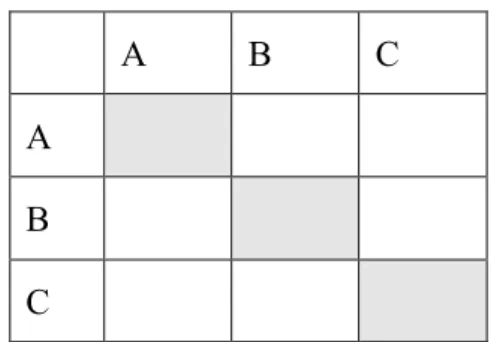
(23) Table 3.1 pair-wise comparisons questionnaire. A. B. C. A B C As the scale ranges incrementally from 1-4 (inclusive), with 1 representing minimal order of impact and 4 representing the maximum order of impact, each respondent will produce a direct-relation matrix Dk , k=1, 2,···, n, and representing the number of respondents. Each element of direct-relation matrix Dk denoted by d ijk , shows the initial direct effects that each criterion exerts outwards and receives from another factor. The matrix D is arranged in the following matrix:. &d11k ! d1kj ! d1kn # ! $ " " ! $" D = $$dik1 ! d ijk ! d ink !! $" " " ! ! $ k k k $%d n1 ! d nj ! d nn !". (1). Next part of the DANP is to attain the average matrix A. It computes an averaged summary of all corresponding values, which we have derived from each respondent’s input. Each value of matrix A is denoted as α ij , and calculated using the Eq. (2):. α ij. ∑ =. n k =1. d ijk. (2). n. Next process of the DANP method is to calculate the initial direct-relation. [ ]. matrix. The initial direct-relation matrix X (i.e., X = xij. !. 16!. n×n. ) can be obtained by.

(24) normalizing 6 the average matrix A through Eqs. (3) and (4), in which all samefactored set values stay equal to zero. (3). X = s× D. s=. 1. (4). MAX1≤i≤n ∑ nj=1 xij. The third step of DANP method is to derive the total relation matrix. Once we obtain the normalized direct-relation matrix X, formula (5) will give the total relation matrix T, in which I represents the identity matrix. Matrix T is the direct/indirect matrix. The factors ij of matrix T denotes the direct and indirect influence from factor i to factor j. T = lim (X + X 2 + ... + X k ) k →∞. = lim X (I + X + X 2 + ... + X k −1 ) = X (I − X ). −1. (5). k →∞. The DANP method’s next step showcases the degrees of influences and relationships of each category. Vector D and vector R, one being a level of influence and one being a level of relation, are defined in Eqs. (6) and (7), respectively. They denote the sum of columns and the sum of rows from total relation matrix T = !"tij #$n×n . n. Di = ∑ tij j =1 n. R j = ∑ t ij j =1. (i = 1,2 ,..., n). (6). (i = 1,2,..., n). (7). The value of (*+ + ,+ )' represents a magnitude of influence a category sends out or receives. A higher value of (*+ + ,+ )'represents an identification towards the central role which exerts a stronger influence on other factors, and assuming a higher priority for consideration. Conversely, the value of (*+ − ,- ) indicates that the factor is subject to influence by surrounding factors. A higher value of (*+ − ,- ). 6. !. Normalizing a factor takes the value and converts it to a relative value, such as a standard. 17!.

(25) means that this factor is influenced more by other factors than the influence it exerts, claiming a lower priority to be considered (Li and Tzeng, 2009; Wu, 2010). 3.2.2 Weight measurements by integrating DEMATEL and ANP Originally, the first step of the ANP is to compare the criteria in whole system to form the super-matrix. According to Saaty (1980, 1996), this is done through pairwise comparisons. The general form of the super-matrix is exemplified below: c. 1 e11 ! e1 m1 e11. c1 e12" c W=. e1 m1 e21 e22 2 " e2 m 2. " en 1. c 2 en"2 enmn. &W11 $ $ $W 21 $ $ $ $ $ " $ $ $W n1 $ %. c. 2 e21 ! e2 n 2. !. c. n en1 ! enmn. W12. !. W1n. W 22. !. W 2n. ". #. ". Wn2. !. W nn. # ! ! ! ! ! ! ! ! ! ! ! ! ". (8). ./ 'denotes the nth cluster, enm denotes the mth element in nth cluster, and Wij = [0] is the principal eigenvector of the influence of the elements compared in the jth cluster to the ith cluster. In addition, if the jth cluster has no influence to the ith cluster, then Wij = [0].. Ou Yang et al. (2008) reveals that the ANP method demonstrates the influence of factors through questionnaires. The dynamic influence relationship implied in the total influence matrix acquired by DEMATEL is similar to the concept of ANP. Because the influence degrees between factors in the total influence matrix 01 are different, all factors of the total-influence matrix 01 should be normalized. The normalized total-influence matrix 02 is calculated as follows:. !. 18!.

(26) (9) α & t11 / d1 ! t1αj / d1 ! t1αn / d1 # &t11s ! t1sj ! $ $ " " " ! $" $ " s α α α ! $ $ = Ts = ti1 / d i ! tij / d i ! tin / d i t i1 ! t ijs ! $ $ " " ! $" " $ " α α α s s $t / d ! t / d ! t / d ! $t nj n nn n" % n1 n % n1 ! t nj. ! t1sn # ! " ! ! t ins ! ! " ! s ! ! t nn ". (10). where t ijs = t ijα / d i Furthermore, the weighted super-matrix 34 such as formula (11) can be calculated by multiplying the un-weighted super-matrix W and the normalized totalinfluence matrix Ts , that is Ww = Ts × W .. & t11s × W11 ! tis1 × Wi1 ! t ns1 × Wn1 # ! $ " " ! $ " Ww = $t1sj × W1 j ! tijs × Wij ! t njs × Wnj ! ! $ " " ! $ " $t s × W ! t s × W ! t s × W ! 1n in un nn nn " % 1n. (11). Finally, the weighted super-matrix can be raised to limiting powers such as formula (12) until it has converged and become a long-term stable super-matrix to obtain the global priority vectors or called the DANP weights (Ou Yang et al., 2008).. !. 19!.

(27) Chapter 4 Standard Operational Procedure This section will provide a straightforward standard operational procedure (SOP) to be available to any researcher seeking way to improve their firm’s decision-making strategy. Improvement will only take effect when unnecessary influences are taken out of the decision making process—in essence, to prevent symptoms of groupthink from negatively skewing a group’s collective direction towards an unfavorable outcome. The role of a facilitator, as mentioned in the previous section, is to perform the due diligence necessary to guide the meeting towards an optimal decision. To achieve as close to an optimal decision as possible, we need to eliminate any elements that will contribute towards biased decisionmaking result, and is only achieved by meticulously adhering to the following steps:. 1.! Define the objective of the decision 2.! List all viable alternatives that may be considered for a final decision 3.! Identify and clearly define all factors that may influence the outcome of the decision. 4.! Consult several credited executives or experts for any additional thoughts regarding the list of factors 5.! Configure survey format based on number of factors used. a.! Decide on point scaling and range b.! Group similar category factors together c.! Align the factors along the X-axis, and also the Y-axis in descending order starting from underneath the X-axis 6.! Arrange a meeting, inviting all case-specific representatives 7.! Administer survey and terminology 8.! Explain each factor thoroughly to avoid errors that might skew results. !. 20!.

(28) 9.! The collected questionnaires are run through the DANP methodology to derive causal diagram and strategy map for each category, and each factorial rank with their respective priorities. a.! Derive initial direct influence matrix by using Eq. (1). Each element of direct-relation matrix Dk denoted by d ijk , shows the initial direct effects that each criterion exerts outwards and receives from another factor b.! Derive the average matrix using the following Eq. (2) c.! Derive the normalized direct influence matrix using Eqs. (3) & (4). d.! Derive the total influence matrix using the following Eq. (5) e.! Derive the given and received influences of the four categories using the Eq. (6) & (7), then graphically plot them on an X-Y axis (* + ,)'on Xaxis, (* − ,) on Y-axis). f.! Find threshold value to filter out erroneous noise. ∑t. ij. / 6 (number of factors). g.! Draw a strategy map to convey relative influences among each factor, omitting values less than threshold value, and divide into 2nd and 3rd quartiles, 7 using values between 2nd-3rd quartiles as having weak influences, and values between 3rd-4th quartiles as having strong influences. Dashed arrows represent weak influences, while solid arrows represent strong influences. h.! Derive the un-weighted super matrix as shown in Eq. (8) i.! Normalize the total influence matrix using Eq. (9) & (10), where. t ijs = t ijα / d i .. 7. !. Quartiles are values that act as cut-off points for a specific range of numbers 21!.

(29) j.! Derive the weighted super matrix by multiplying the un-weighted supermatrix 3 and the normalized total-influence matrix as in Eq. (11). k.! Derive the limiting super matrix by raising the weighted super-matrix to limiting powers. 10.!Based on the weights derived from the DANP methodology, an optimal location can be chosen from a set of feasible alternatives. By multiplying the weights to each point for each factor, the total sum for each alternative can be derived. The highest score should be the optimal choice for the case. 11.!The executive, considering the priority of factors, will make a final decision upon which option to move forward with. Unsurprisingly, the optimal choice suggested by the methodology may not be chosen, because an undisclosed factor known to the executive could have weighed in on his decision.. These elements not only pose a silent threat, but are also very prevalent among firms in general. Symptoms of groupthink, bounded rationality, and escalating commitment are a few among those recognized to negatively influence decision making in a typical groupthink setting. Therefore, by carefully applying the following SOP to any specific case, a researcher will be equipped with a systematic and practical tool that incorporates DANP methodology to overcome these symptoms of groupthink.. !. 22!.

(30) Chapter 5 A case study This recent case study is a literal account attempting to apply a revolutionary methodology to a practical, real-life event. The methodology is employed due to a prevalent and growing concern towards decision making. In most groupthink settings, biases form within individuals and groups. These groupthink symptoms have a high potential to misguide the group as a whole towards a less-favorable decision path. In the following case, a sub-unit of the company dealing with advanced packaging solutions wished to expand its production lines to satisfy a growing demand of sales. With too many factors that may influence the outcome of the company’s decision, a facilitator was called to manage and overlook the case. To kickoff the investigation, the facilitator consulted all key experts with certified expertise towards the issue, in which they were asked to contribute factors attributable to this decision. These key experts included managerial and VP-level executives with considerable experience relevant to the decision topic. The factors varied sporadically along the importance spectrum, but to prevent a skew of data, the factors were not excluded from the questionnaire. Next, a meeting was called, and the executives were briefed on each factor in table 5.1, and were asked to respond to two parts of the survey: The first section asked for comparisons among the following categories: machinery, finance, environment, and location. The second section asked for comparisons among all individual factors. Grouping these factors into four categories allowed the hybrid MCDM (Multiple Criteria Decision Making) model identify the interrelationship between each category and the degree of relative importance among each factor within its category.. !. 23!.

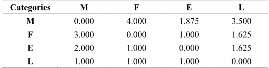
(31) Table%4.1%Defined%terminology%for%selected%factors% Table 5.1 Definition of key factors. (Sources%obtained%from%various%highElevel%executives) Categories. Machine Financials Environment Location. Selected.evaluation.indexes. Description. (M1)%Machine%Count. Quantity%of%deviceEspecific%machines%to%fulfill%demand. (M2)%Tooling (M3)%Utilization. Specific%tools%and%kits%that%enable%a%specific%demand%to%be%fulfilled Percentage%of%total%capacity%allocated%for%production. (M4)%UPH. Machine’s%capacity%of%units%produced%per%hour. (M5)%Machine%Compatibility. MachineEtype%limitations%for%specific%deviceEspecific%operations. (M6)%OEE. Key%production%metric%that%provides%the%ratio%of%actual%productivity%in% comparison%to%the%ideal. (F1)%Profit%Margin. Ratio%of%net%income%to%total%revenue%. (F2)%Forecast%. CustomerEprovision%of%data%that%serves%as%a%rough%prediction%of%future%orders. (F3)%Headcount. Resource%used%to%hire%additional%manpower. (E1)%Wastewater. GovernmentEspecified%criteria%restricting%amounts%of%various%contaminated% water%to%be%released%into%the%environment. (E2)%Energy%Resources. Limitations%in%available%supply%of%electricity%and/or%gasses%as%required%resources% for%production%. (E3)%Emissions. Restrictions%concerning%the%allowable%gasEstate%waste%that%is%released%into%the% environment. (L1)%Space. Volume%of%required%space%required%to%fulfill%additional%manufacturing%demands. (L2)%Clean%Room%Criteria. Adherence%to%ISO%standards%to%be%met%for%each%productive%environment. (L3)%Customer%Consent. Adherence%to%customer%inquiry/requests%regarding%the%production%of%their%units. (L4)%Safety%/%Security. Measures%of%safety/security%installments%to%prevent%liabilities%towards%the% company%or%to%its%employees. (All definitions sourced from high-level executives, holding Ph.Ds, with positions of “Dep.Director”level and upwards). 5.1 Measuring relationships among categories The initial direct influence matrix A is summarized in Table 5.2. Table 5.2 The initial direct influence matrix A of the four categories. !. Categories. M. F. E. L. M F E L. 0.000 3.000 2.000 1.000. 4.000 0.000 1.000 1.000. 1.875 1.000 0.000 1.000. 3.500 1.625 1.625 0.000. 24!.

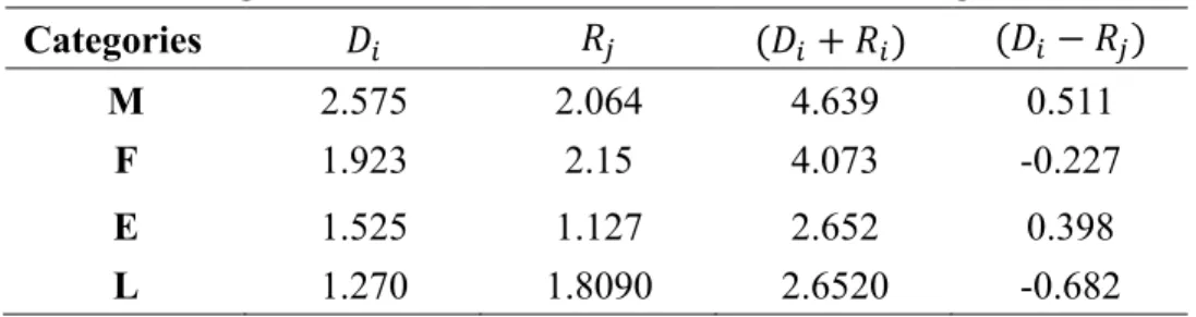
(32) The normalized direct influence matrix X and the total influence matrix T were calculated by using Eq. (3) and Eq. (5), respectively, as shown in Table 5.3 and Table 5.4.. Table 5.3 The normalized direct influence matrix X of the four categories. Categories. M. F. E. L. M F E L. 0.000 1.280 0.853 0.427. 1.707 0.000 0.427 0.427. 0.800 0.427 0.000 0.427. 1.493 0.693 0.693 0.000. Table. 5.4 The total influence matrix T of the four categories. Categories. M. F. E. L. M F E L. 2.575 1.923 1.525 1.127. 2.064 2.15 1.127 1.809. 4.639 4.073 2.652 2.936. 0.511 -0.227 0.398 -0.682. Table 5.5 uses Equations (6) and Equations (7) to find the degrees of given and received influences at play among the four categories. 5.5 The given and received influences of the four categories ,(*+ − ,- ) Categories *+ (*+ + ,+ )' Table. M F. 2.575 1.923. 2.064 2.15. 4.639 4.073. 0.511 -0.227. E L. 1.525 1.270. 1.127 1.8090. 2.652 2.6520. 0.398 -0.682. 5.1.1 The ranking of (D8 + R 8 )' and (D8 − R : ) The results, as shown revealed that the highest (*+ + ,+ )' value presented the most relativity among the other categories, and is associated with a central role. The “machine” category in this study dominated the central role category; whereas, !. 25!.

(33) the location category came in last with the lowest (*+ − ,- ) value, indicating that it receives the strongest influence from the other factors.. 5.1.2 The Causal Diagram According to Table 5.5, the causal diagram of the total influence is depicted as Fig.5.1. The category with the highest positive values of (*+ + ,+ ) show that it carries the most weight for deciding whether to invest in capital expenditure. However, the financial category is a close runner-up, and should undoubtedly share a similar order of importance. The location category, lacking a power to influence other categories, was not prioritized. Thus, machine-related issues were considered as a priority category for optimal decision making in this case.. 5.1.3 The Strategy Map A strategy map was constructed from Table 5.4 and shown as Fig. 5.2. A threshold value should be decided to eliminate insignificant noise, which resulted from our DEMATEL analysis. For this research, the threshold value is computed from the elements of matrix T by. !. 26!.

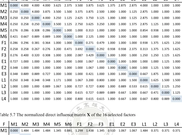
(34) ∑t. ij. /16 = 0.4667. To distinguish further levels of influence, the second quartile (0.419) and third quartile (0.908) were set as second and third parameter limits to specify ranges to be assumed as either weak or strong in its influence toward other categories. In Fig. 5.2, the dotted lines indicate weak influence among the categories whereas the solid bold lines indicate a strong exertion of influence. For this capacity expenditure-related decision, it can be observed from Fig. 5.2 that the machine category is the prime factor, which carries the strongest influence on the other categories, while the location perspective is the main effect factor, which serves only as a recipient of influence, not making the threshold to be considered as a significant influencer towards others.. 5.2 Weight measuring among factors DEMATEL and ANP were used in conjunction to formulate the relative weights of factors that effect capacity expansion. As mentioned previously, the initial direct influence matrix A of the 16 selected factors can be obtained by Eq. (2) The normalized direct influence matrix X of the 16 selected factors and the total !. 27!.

(35) influence matrix T of the 16 selected factors can be computed by Eq. (3) and Eq. (5), respectively, and presented in Table 5.6 and Table 5.7 Table 5.6 The initial direct influence matrix A of the 16 selected factors. F M1 M2 M3 M4 M5 M6 F1 F2 F3 E1 E2 E3 L1 L2 L3 L4 M1 0.000 4.000 4.000 4.000 3.625 2.375 3.500 3.875 3.625 1.375 2.875 2.875 4.000 1.000 1.000 1.000 M2 0.250 0.000 4.000 3.875 3.500 1.500 3.375 3.875 2.500 1.000 1.000 1.125 2.875 1.000 1.000 1.000 M3 0.250 0.250 0.000 4.000 3.250 1.125 2.625 3.750 3.125 1.000 1.000 1.125 2.875 1.000 1.000 1.000 M4 0.250 0.258 0.250 0.000 3.500 1.125 2.750 3.625 3.250 1.000 1.000 1.375 2.875 1.125 1.000 1.000 M5 0.276 0.286 0.308 0.286 0.000 1.000 1.000 0.313 1.000 1.000 1.000 1.000 0.854 0.938 1.000 1.000 M6 0.421 0.667 0.889 0.889 1.000 0.000 1.000 2.125 1.000 1.000 1.000 1.000 1.000 1.000 1.000 1.000 F1 0.286 0.296 0.381 0.364 1.000 1.000 0.000 0.271 0.479 1.000 1.000 1.000 0.938 1.375 1.625 1.250 F2 0.258 0.258 0.267 0.276 3.200 0.471 3.692 0.000 0.292 0.938 0.938 2.375 0.313 1.375 1.375 1.625 F3 0.276 0.400 0.320 0.308 1.000 1.000 2.087 3.429 0.000 1.000 1.000 1.000 1.250 1.250 1.125 1.625 E1 0.727 1.000 1.000 1.000 1.000 1.000 1.000 1.067 1.000 0.000 1.000 1.000 1.000 1.000 1.125 1.000 E2 0.348 1.000 1.000 1.000 1.000 1.000 1.000 1.067 1.000 1.000 0.000 1.000 1.000 1.125 1.500 1.500 E3 0.348 0.889 0.889 0.727 1.000 1.000 1.000 0.421 1.000 1.000 1.000 0.000 0.667 1.875 1.000 1.000 L1 0.250 0.348 0.348 0.348 1.171 1.000 1.067 3.200 0.800 1.000 1.000 1.500 0.000 1.625 1.500 1.500 L2 1.000 1.000 1.000 0.889 1.067 1.000 0.727 0.727 0.800 1.000 0.889 0.533 0.615 0.000 2.125 1.250 L3 1.000 1.000 1.000 1.000 1.000 1.000 0.615 0.727 0.889 0.889 0.667 1.000 0.667 0.471 0.000 1.125 L4 1.000 1.000 1.000 1.000 1.000 1.000 0.800 0.615 0.615 1.000 0.667 1.000 0.667 0.800 0.889 0.000 Table 5.7 The normalized direct influence matrix X of the 16 selected factors. F M1 M2 M3 M4 M5 M6 F1 F2 F3 E1 E2 E3 L1 L2 L3 L4 M1 0.000 1.484 1.484 1.484 1.345 0.881 1.299 1.438 1.345 0.510 1.067 1.067 1.484 0.371 0.371 0.371 M2 0.093 0.000 1.484 1.438 1.299 0.557 1.252 1.438 0.928 0.371 0.371 0.417 1.067 0.371 0.371 0.371 M3 0.093 0.093 0.000 1.484 1.206 0.417 0.974 1.391 1.159 0.371 0.371 0.417 1.067 0.371 0.371 0.371 M4 0.093 0.096 0.093 0.000 1.299 0.417 1.020 1.345 1.206 0.371 0.371 0.510 1.067 0.417 0.371 0.371 M5 0.102 0.106 0.114 0.106 0.000 0.371 0.371 0.116 0.371 0.371 0.371 0.371 0.317 0.348 0.371 0.371 M6 0.156 0.247 0.330 0.330 0.371 0.000 0.371 0.788 0.371 0.371 0.371 0.371 0.371 0.371 0.371 0.371 F1 0.106 0.110 0.141 0.135 0.371 0.371 0.000 0.100 0.178 0.371 0.371 0.371 0.348 0.510 0.603 0.464 F2 0.096 0.096 0.099 0.102 1.187 0.175 1.370 0.000 0.108 0.348 0.348 0.881 0.116 0.510 0.510 0.603 F3 0.102 0.148 0.119 0.114 0.371 0.371 0.774 1.272 0.000 0.371 0.371 0.371 0.464 0.464 0.417 0.603 E1 0.270 0.371 0.371 0.371 0.371 0.371 0.371 0.396 0.371 0.000 0.371 0.371 0.371 0.371 0.417 0.371 E2 0.129 0.371 0.371 0.371 0.371 0.371 0.371 0.396 0.371 0.371 0.000 0.371 0.371 0.417 0.557 0.557 E3 0.129 0.330 0.330 0.270 0.371 0.371 0.371 0.156 0.371 0.371 0.371 0.000 0.247 0.696 0.371 0.371 L1 0.093 0.129 0.129 0.129 0.434 0.371 0.396 1.187 0.297 0.371 0.371 0.557 0.000 0.603 0.557 0.557 L2 0.371 0.371 0.371 0.330 0.396 0.371 0.270 0.270 0.297 0.371 0.330 0.198 0.228 0.000 0.788 0.464 L3 0.371 0.371 0.371 0.371 0.371 0.371 0.228 0.270 0.330 0.330 0.247 0.371 0.247 0.175 0.000 0.417 L4 0.371 0.371 0.371 0.371 0.371 0.371 0.297 0.228 0.228 0.371 0.247 0.371 0.247 0.297 0.330 0.000. !. 28!.

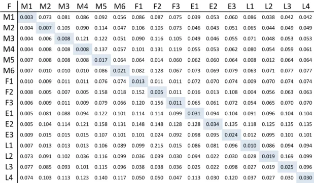
(36) Table 5.8 The total influence matrix T of the selected 16 factors. F M1 M2 M3 M4 M5 M6 F1 F2 F3 E1 E2 E3 L1 L2 L3 L4 M1 0.003 0.073 0.081 0.086 0.092 0.056 0.086 0.087 0.075 0.039 0.053 0.060 0.086 0.038 0.042 0.042 M2 0.004 0.007 0.105 0.090 0.114 0.047 0.106 0.105 0.073 0.046 0.043 0.051 0.065 0.044 0.049 0.049 M3 0.004 0.006 0.008 0.121 0.122 0.051 0.090 0.116 0.105 0.049 0.046 0.055 0.071 0.048 0.053 0.053 M4 0.004 0.008 0.008 0.008 0.137 0.057 0.101 0.131 0.119 0.055 0.053 0.062 0.080 0.054 0.059 0.061 M5 0.007 0.008 0.008 0.008 0.017 0.064 0.064 0.014 0.060 0.062 0.060 0.064 0.008 0.012 0.064 0.064 M6 0.007 0.010 0.010 0.010 0.086 0.021 0.082 0.128 0.067 0.073 0.069 0.079 0.063 0.071 0.077 0.077 F1 0.010 0.009 0.011 0.011 0.076 0.074 0.013 0.011 0.011 0.072 0.070 0.074 0.009 0.070 0.074 0.074 F2 0.008 0.005 0.007 0.005 0.158 0.018 0.152 0.005 0.011 0.016 0.013 0.108 0.004 0.056 0.063 0.063 F3 0.006 0.009 0.011 0.009 0.079 0.066 0.120 0.156 0.011 0.065 0.061 0.072 0.054 0.065 0.070 0.070 E1 0.005 0.081 0.088 0.094 0.122 0.101 0.114 0.114 0.099 0.031 0.094 0.104 0.091 0.096 0.104 0.104 E2 0.005 0.104 0.114 0.121 0.158 0.131 0.148 0.148 0.128 0.128 0.034 0.135 0.118 0.125 0.135 0.135 E3 0.009 0.015 0.015 0.015 0.107 0.101 0.101 0.024 0.092 0.098 0.095 0.024 0.012 0.095 0.101 0.101 L1 0.007 0.013 0.013 0.013 0.106 0.089 0.099 0.215 0.015 0.086 0.081 0.096 0.010 0.086 0.094 0.094 L2 0.073 0.091 0.102 0.036 0.116 0.099 0.036 0.039 0.030 0.094 0.022 0.030 0.028 0.019 0.169 0.099 L3 0.077 0.085 0.093 0.101 0.115 0.096 0.038 0.038 0.036 0.025 0.022 0.098 0.027 0.019 0.025 0.096 L4 0.074 0.103 0.113 0.123 0.140 0.117 0.050 0.050 0.047 0.113 0.030 0.120 0.037 0.027 0.030 0.030. The dynamic influence relationship between factors resulted from constructing its degree of importance in an un-weighted super matrix (Table 5.9), and using Eq. (8).. Table 5.9 The un-weighted super matrix of the 16 selected factors. F M1 M2 M3 M4 M5 M6 F1 F2 F3 E1 E2 E3 L1 L2 L3 L4 M1 0.015 0.027 0.037 0.044 0.106 0.070 0.090 0.087 0.058 0.065 0.054 0.076 0.042 0.058 0.074 0.075 M2 0.016 0.028 0.032 0.042 0.105 0.070 0.086 0.078 0.057 0.064 0.053 0.077 0.039 0.056 0.074 0.074 M3 0.017 0.030 0.034 0.032 0.104 0.071 0.089 0.080 0.053 0.065 0.053 0.079 0.038 0.057 0.076 0.076 M4 0.019 0.033 0.037 0.036 0.100 0.073 0.087 0.073 0.044 0.066 0.053 0.082 0.033 0.057 0.078 0.078 M5 0.014 0.028 0.032 0.033 0.064 0.049 0.049 0.047 0.035 0.042 0.033 0.050 0.028 0.039 0.045 0.048 M6 0.022 0.040 0.045 0.043 0.102 0.074 0.082 0.064 0.046 0.063 0.047 0.078 0.033 0.055 0.075 0.075 F1 0.019 0.037 0.042 0.040 0.072 0.058 0.054 0.048 0.045 0.050 0.036 0.054 0.031 0.038 0.056 0.057 F2 0.018 0.025 0.028 0.026 0.059 0.057 0.041 0.025 0.035 0.051 0.040 0.047 0.016 0.033 0.052 0.053 F3 0.021 0.036 0.041 0.039 0.102 0.068 0.078 0.056 0.045 0.060 0.046 0.078 0.030 0.055 0.073 0.074 E1 0.030 0.050 0.063 0.068 0.156 0.106 0.123 0.116 0.082 0.099 0.073 0.111 0.059 0.081 0.109 0.110 E2 0.039 0.063 0.079 0.085 0.198 0.135 0.156 0.147 0.103 0.120 0.100 0.142 0.074 0.103 0.139 0.140 E3 0.027 0.050 0.057 0.055 0.103 0.082 0.077 0.077 0.056 0.071 0.052 0.084 0.047 0.056 0.081 0.081 L1 0.027 0.047 0.053 0.051 0.126 0.082 0.098 0.060 0.058 0.071 0.053 0.094 0.039 0.064 0.088 0.089 L2 0.026 0.047 0.060 0.072 0.113 0.078 0.086 0.085 0.068 0.062 0.055 0.086 0.052 0.052 0.066 0.077 L3 0.015 0.030 0.041 0.051 0.102 0.067 0.085 0.080 0.069 0.066 0.055 0.070 0.047 0.052 0.065 0.066 L4 0.013 0.034 0.047 0.058 0.123 0.081 0.109 0.103 0.087 0.073 0.072 0.084 0.061 0.070 0.087 0.088. The weighted super-matrix Ww is then calculated by multiplying the unweighted super-matrix Ww by itself repeatedly until a normalized total-influence !. 29!.

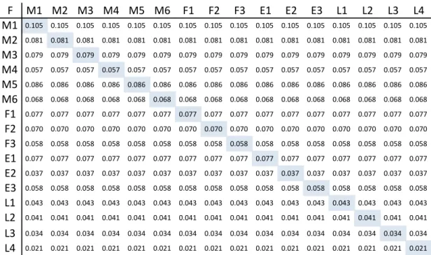
(37) matrix T with Eq. (11) forms based on the degree of influence of each dimension (Table 5.10).. Table 5.10 The weighted super matrix of the 16 selected factor. F M1 M2 M3 M4 M5 M6 F1 M1 0.015 0.027 0.037 0.044 0.106 0.070 0.090 M2 0.016 0.028 0.032 0.042 0.105 0.070 0.086 M3 0.017 0.030 0.034 0.032 0.104 0.071 0.089 M4 0.019 0.033 0.037 0.036 0.100 0.073 0.087 M5 0.014 0.028 0.032 0.033 0.064 0.049 0.049 M6 0.022 0.040 0.045 0.043 0.102 0.074 0.082 F1 0.019 0.037 0.042 0.040 0.072 0.058 0.054 F2 0.018 0.025 0.028 0.026 0.059 0.057 0.041 F3 0.021 0.036 0.041 0.039 0.102 0.068 0.078 E1 0.030 0.050 0.063 0.068 0.156 0.106 0.123 E2 0.039 0.063 0.079 0.085 0.198 0.135 0.156 E3 0.027 0.050 0.057 0.055 0.103 0.082 0.077 L1 0.027 0.047 0.053 0.051 0.126 0.082 0.098 L2 0.026 0.047 0.060 0.072 0.113 0.078 0.086 L3 0.015 0.030 0.041 0.051 0.102 0.067 0.085 L4 0.013 0.034 0.047 0.058 0.123 0.081 0.109. F2. F3. E1. E2. E3. L1. L2. L3. L4. 0.087 0.058 0.065 0.054 0.076 0.042 0.058 0.074 0.075 0.078 0.057 0.064 0.053 0.077 0.039 0.056 0.074 0.074 0.080 0.053 0.065 0.053 0.079 0.038 0.057 0.076 0.076 0.073 0.044 0.066 0.053 0.082 0.033 0.057 0.078 0.078 0.047 0.035 0.042 0.033 0.050 0.028 0.039 0.045 0.048 0.064 0.046 0.063 0.047 0.078 0.033 0.055 0.075 0.075 0.048 0.045 0.050 0.036 0.054 0.031 0.038 0.056 0.057 0.025 0.035 0.051 0.040 0.047 0.016 0.033 0.052 0.053 0.056 0.045 0.060 0.046 0.078 0.030 0.055 0.073 0.074 0.116 0.082 0.099 0.073 0.111 0.059 0.081 0.109 0.110 0.147 0.103 0.120 0.100 0.142 0.074 0.103 0.139 0.140 0.077 0.056 0.071 0.052 0.084 0.047 0.056 0.081 0.081 0.060 0.058 0.071 0.053 0.094 0.039 0.064 0.088 0.089 0.085 0.068 0.062 0.055 0.086 0.052 0.052 0.066 0.077 0.080 0.069 0.066 0.055 0.070 0.047 0.052 0.065 0.066 0.103 0.087 0.073 0.072 0.084 0.061 0.070 0.087 0.088. The limiting super matrix is used to calculate the weight of each factor by Eq. (12), as illustrated in Table 5.11. Table 5.11 The limiting super matrix of the 16 selected factors. F M1 M2 M3 M4 M5 M6 F1 F2 F3 E1 E2 E3 L1 L2 L3 L4 M1 0.105 0.105 0.105 0.105 0.105 0.105 0.105 0.105 0.105 0.105 0.105 0.105 0.105 0.105 0.105 0.105 M2 0.081 0.081 0.081 0.081 0.081 0.081 0.081 0.081 0.081 0.081 0.081 0.081 0.081 0.081 0.081 0.081 M3 0.079 0.079 0.079 0.079 0.079 0.079 0.079 0.079 0.079 0.079 0.079 0.079 0.079 0.079 0.079 0.079 M4 0.057 0.057 0.057 0.057 0.057 0.057 0.057 0.057 0.057 0.057 0.057 0.057 0.057 0.057 0.057 0.057 M5 0.086 0.086 0.086 0.086 0.086 0.086 0.086 0.086 0.086 0.086 0.086 0.086 0.086 0.086 0.086 0.086 M6 0.068 0.068 0.068 0.068 0.068 0.068 0.068 0.068 0.068 0.068 0.068 0.068 0.068 0.068 0.068 0.068 F1 0.077 0.077 0.077 0.077 0.077 0.077 0.077 0.077 0.077 0.077 0.077 0.077 0.077 0.077 0.077 0.077 F2 0.070 0.070 0.070 0.070 0.070 0.070 0.070 0.070 0.070 0.070 0.070 0.070 0.070 0.070 0.070 0.070 F3 0.058 0.058 0.058 0.058 0.058 0.058 0.058 0.058 0.058 0.058 0.058 0.058 0.058 0.058 0.058 0.058 E1 0.077 0.077 0.077 0.077 0.077 0.077 0.077 0.077 0.077 0.077 0.077 0.077 0.077 0.077 0.077 0.077 E2 0.037 0.037 0.037 0.037 0.037 0.037 0.037 0.037 0.037 0.037 0.037 0.037 0.037 0.037 0.037 0.037 E3 0.058 0.058 0.058 0.058 0.058 0.058 0.058 0.058 0.058 0.058 0.058 0.058 0.058 0.058 0.058 0.058 L1 0.043 0.043 0.043 0.043 0.043 0.043 0.043 0.043 0.043 0.043 0.043 0.043 0.043 0.043 0.043 0.043 L2 0.041 0.041 0.041 0.041 0.041 0.041 0.041 0.041 0.041 0.041 0.041 0.041 0.041 0.041 0.041 0.041 L3 0.034 0.034 0.034 0.034 0.034 0.034 0.034 0.034 0.034 0.034 0.034 0.034 0.034 0.034 0.034 0.034 L4 0.021 0.021 0.021 0.021 0.021 0.021 0.021 0.021 0.021 0.021 0.021 0.021 0.021 0.021 0.021 0.021. !. 30!.

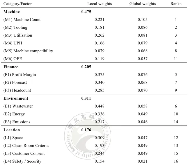
(38) 5.2.1 The ranking of the factors The local and the global weights of the factors, which were developed via the DANP approach can be listed as Table 5.11. Through the limiting super matrix of ANP approach, we can obtain the global weight of each factor. Furthermore, the importance of factor under the same category is summed up to get the local weight of that category. The local weights represent the importance that each factor in comparison to the other factor in the same category. The global weights help us understand the overall absolute weights of individual factors. The purpose of weight measuring is so that if multiple sets of viable solutions were presented, an optimal choice can be made based on an this objectively ranked dataset, as shown below. We can infer from the table below that within the four major categories, machinery related factors carry a substantial priority over the other categories. However, the local weights within this category are spread relatively evenly throughout, which further strengthens the position, because the data emphasizes the category as a group resulted from its strength in number of factors, not skewed by any outliers.. !. 31!.

(39) Table 5.12 Weights and ranking Category/Factor Machine. Global weights. Ranks. 0.475. (M1) Machine Count. 0.221. 0.105. 1. (M2) Tooling. 0.181. 0.086. 2. (M3) Utilization. 0.262. 0.081. 3. (M4) UPH. 0.166. 0.079. 4. (M5) Machine compatibility. 0.079. 0.068. 8. (M6) OEE. 0.119. 0.057. 11. (F1) Profit Margin. 0.375. 0.076. 5. (F2) Forecast. 0.340. 0.068. 7. (F3) Headcount. 0.285. 0.070. 9. (E1) Wastewater. 0.448. 0.058. 6. (E2) Energy. 0.336. 0.049. 10. (E3) Emissions. 0.217. 0.046. 14. (L1) Space. 0.309. 0.047. 12. (L2) Clean Room Criteria. 0.193. 0.049. 13. (L3) Customer Consent. 0.244. 0.049. 15. (L4) Safety / Security. 0.154. 0.021. 16. Finance. Environment. Location. !. Local weights. 0.205. 0.311. 0.176. 32!.

(40) The tables 5.13 and 5.14 show several made-up locations, where each factors were ranked according to its contextual characteristics. The points were scaled according to increasing favorability. To select the best location for the capacity expansion project, the global weights, or priority ratio derived from the DANP evaluation, are applied onto each location’s factorial attributes. Each weighted factor was then summed up, revealing the total weighted sum of each location as in Table 5.14. Assuming that location alternatives differed only in the Environment and Location categories, we disregarded them completely. According to this case, it is apparent that the optimal choice by applying the steps provided by the SOP is to expand capacity at Azeroth.. !. 33!.

(41) Chapter 6 Concluding Remarks 6.1 Conclusion To emphasize the focus of this research, past literatures have demonstrated the importance of eliminating biases when making company-risking decisions. Biases such as groupthink, bounded rationality, and the theory of escalating commitment have been observed and repetitively diagnosed as causes and symptoms reoccurring with high prevalence in the past, evoking other researchers to investigate even further. However, a chosen methodology, a hybrid of ANP and DEMETAL (DANP), has demonstrated and proven to be a systematic solution towards optimal decision-making. In the case study, we combined the practicality of the SOP with a theoretical methodology to overcome symptoms of groupthink. The SOP allows for a researcher to arrive at a concise set of data evaluated to directly point at the optimal choice for any multiple criterial decision. After a thorough investigation via surveys, we have broken down each factor’s importance in relation to each other, which within the methodology removed existing biases that could have resulted in a different, less optimal decision for the company.. 6.2 Discussion Results from the case study concluded that the machine category played the most important role and should be considered a top priority. The results showed the category to be a high exertion of influence among all other categories. However, it is imperative to keep note that these factors and categories of importance only apply to this case alone, since factors can have a drastic difference depending on its innumerable contextual possibilities, such as the country laws, economic fluctuations, availability of equipment needed in the proposed country.. !. 34!.

(42) For this company dealing with advanced packaging solutions, although it may have seemed like common knowledge to experienced executives that machines were the most important among other categories, and that location will never have been a top priority, we needed more than just a few voices for a confident solution. Also, this may also be a way to have the opposition gain a greater understanding in the breakdown of this issue. On the other hand, a possibility could arise where new manufacturing methods and breakthroughs have been proposed to improve on existing thoughts and experiences. If so, perhaps the scales would have tipped toward a heavier weight on the less obvious, location for example. Without a systematic way to break individual factors down, any factor could be biased to sound important. Backed by previous research and literature, a critical foundation for a better decision-making path.. !. 35!.

(43) References Arkes, H. & C. Blumer, (1985), The psychology of sunk cost, Organizational Behavior and Human Decision Processes, 35, 125-140. Arthur, B.W., (1994), Inductive reasoning and bounded rationality, The American Economic Review, 84(2), 406-411. Bazerman, M.H., T. Guiliano, & A. Appelman, (1984), Escalation of commitment in individual and group decision making, Organizational Behavior and Human Performance, 33, 141-152. Brockner, J. & J.Z. Rubin, (1985), Entrapment in escalating conflicts: A Social Psychological Analysis, Springer Science & Business Media, 2012 Carpenter, M.A., Geletkanycz, M.A., & Sanders, W.G., (2004), The upper echelons revisited: Antecedents, elements, and consequences of top management team composition, Journal of Management, 60(6), 749-778. Edman, J., (2006), Group composition and groupthink in a business game, Developments in Business Simulation and Experiential Learning, 33, 278- 283. Gabus, A. & E. Fontela, (1972), World problems, an invitation to further thought within the framework of DEMATEL, Geneva, Switzerland: Battelle Geneva Research Center. Goll, I., Sambharya, R. B., and L.A. Tucci (2001), Top management team composition,. corporate. ideology. and. firm. performance,. Management. International Review, 41(2), 109-129. Hambrick, D. C., Cho, T. S., & M. Chen, (1996), The influence of top management team heterogeneity on firms’ competitive moves, Administrative Science Quarterly, 41, 659-685. Hambrick, D. & P. Mason, (1984), Upper echelons: The organization as a reflection of its top managers, Academy of Management Review, 9, 193-206. !. 36!.

(44) Hart, P., (1991), Irving L. Janis' victims of groupthink, Political Psychology, 12(2), 247-278. Henry, R.A., (1995), Improving group judgment accurately: Information sharing and determining the best member, Organizational Behavior and Human Decision Processes, 62, 190-197. Janis, I.L., (1972), Victims of Groupthink. New York: Houghton Mifflin. Kahneman, D. & A. Tversky, (1984), Choices, values and frames, American Psychologist, 39, 341-350. Kolbe, M. & M. Boos, (2008), Facilitating group decision-making: Facilitator's subjective theories on group coordination. Forum: Qualitative Social Research, 10(1), article. 28 <http://www.qualitative-research.net/index.php/fqs/- article/view/1244/2692> Lang, S.S., (2006), 'Mindless autopilot' drives people to dramatically underestimate how many daily food decisions they make, Cornell Chronicle: Daily news. <http://www.news.cornell.edu/stories/2006/12/mindless-autopilot-drives-peopleunderestimate-food-decisions, 20150520> Mieghem, V.J., (2003), Capacity management, investment and hedging: Review and recent developments. Manufacturing & Service Operations Management, 5(4), 269-302. Miltenburg, J., (1995), Manufacturing Strategy: How to Formulate and Implement a Winning Plan, Portland, OR, Productivity Press. Murray, A.I., (1989), Top management group heterogeneity and firm performance, Strategic Management Journal, 10, 125-141. Noelle-Neumann, E., (1974), The spiral of silence: a theory of public opinion, Journal of Communication, 24, 43-51.. !. 37!.

(45) Ou Yang, Y. P., H. M. Shieh, J. D. Leu, and G. H. Tzeng, (2008), A novel hybrid MCDM model combined with DEMATEL and ANP with applications, International Journal of Operations Research, 5(3), 160-168. Packer, D.J., (2008), On being both with us and against us: A normative conflict model of dissent in social groups, Personality and Social Psychology Review, 12, 50-72. Saaty, T. L., (1980), The Analytic Hierarchy Process, New York: McGraw-Hill. ____, T. L., (1996), Decision Making with Dependence and Feedback: Analytic Network Process, Pittsburgh: RWS Publications. Sumrit, D & P. Anuntavoranich, (2013), Using DEMATEL method to analyze the casual relations on technical innovation capability evaluation factors in Thai technology based firms, International Transaction Journal of Engineering, Management, and Applied Sciences and Technologies, 4(2), 81-103. Teger, A.I., (1980), Too Much Invested to Quit, New York: Pergamon Press. Terry, D.J., & M.A. Hogg, (1996), Group norms and the attitude-behavior relationship: A role for group identification, Personality and Social Psychology Bulletin, 22, 776-795. Von Bergen, C.W. and R.J. Kirk, (1978), Groupthink: When too many heads spoil the decision, Management Review, 67(3), 44-49. West, C.T. Jr. & C.R. Schwenk, (1996), Top management team strategic consensus, demographic homogeneity and firm performance, Strategic Management Journal, 17(7), 571-576. White, G., (1993), Escalating commitment in individual and group decision making: a prospect theory approach, Organizational and Human Decision Processes, 54, 430-455.. !. 38!.

(46) Appendix The questionnaire of this research is divided into four parts: A. Example of questionnaire; B. Description of key factors C. Comparison of the impact of the four categories; D. Comparison of the impact of the factors; E. Personal Profiles of sourced experts. A. Example of questionnaire A. B. C. 3. A B C. 1. Note: 1. Low impact; 2. Medium impact; 3. High impact; 4. Very high impact. !. 39!.

(47) Table%4.1%Defined%terminology%for%selected%factors% B. Definitions of key factors (Sources%obtained%from%various%highElevel%executives) Categories. Machine Financials Environment Location. Selected.evaluation.indexes. Description. (M1)%Machine%Count. Quantity%of%deviceEspecific%machines%to%fulfill%demand. (M2)%Tooling (M3)%Utilization. Specific%tools%and%kits%that%enable%a%specific%demand%to%be%fulfilled Percentage%of%total%capacity%allocated%for%production. (M4)%UPH. Machine’s%capacity%of%units%produced%per%hour. (M5)%Machine%Compatibility. MachineEtype%limitations%for%specific%deviceEspecific%operations. (M6)%OEE. Key%production%metric%that%provides%the%ratio%of%actual%productivity%in% comparison%to%the%ideal. (F1)%Profit%Margin. Ratio%of%net%income%to%total%revenue%. (F2)%Forecast%. CustomerEprovision%of%data%that%serves%as%a%rough%prediction%of%future%orders. (F3)%Headcount. Resource%used%to%hire%additional%manpower. (E1)%Wastewater. GovernmentEspecified%criteria%restricting%amounts%of%various%contaminated% water%to%be%released%into%the%environment. (E2)%Energy%Resources. Limitations%in%available%supply%of%electricity%and/or%gasses%as%required%resources% for%production%. (E3)%Emissions. Restrictions%concerning%the%allowable%gasEstate%waste%that%is%released%into%the% environment. (L1)%Space. Volume%of%required%space%required%to%fulfill%additional%manufacturing%demands. (L2)%Clean%Room%Criteria. Adherence%to%ISO%standards%to%be%met%for%each%productive%environment. (L3)%Customer%Consent. Adherence%to%customer%inquiry/requests%regarding%the%production%of%their%units. (L4)%Safety%/%Security. Measures%of%safety/security%installments%to%prevent%liabilities%towards%the% company%or%to%its%employees. (All definitions sourced from high-level executives, holding Ph.Ds, with positions of “Dep.Director”level and upwards). C. Comparison of the impact of the 4 categories. Machine Finance Environment Location Note: 1. Minimal impact; 2. Medium impact; 3. High impact; 4. Very high impact. !. 40!. Location. Environment. Finance. Machine. Category.

(48) D. Comparison of the impact of the 16 factors. E. Personal Profiles 1. Gender: □Male □Female 2. Educational background: □Bachelors □Master □Doctorate 3. Current Title: □Manager □Deputy Director □Director □Senior Director □ VP 4. Seniority: □Less than 5 years □5 10 years □10 15 years □15 20 years □ Over 20 years. !. 41!.

(49)