國 立 交 通 大 學
電 子 工 程 學 系 電 子 研 究 所
博 士 論 文
BICM-OFDM 系統
在時變通道下之干擾
消除和多樣性分析
BICM-OFDM Systems over Time-Varying
Channels: ICI Cancellation and Diversity
Order Analysis
研
究
生 : 林欣德
指 導 教 授 : 桑梓賢
林大衛
BICM-OFDM 系統
在時變通道下之干擾消除和多樣性分析
BICM-OFDM Systems over Time-Varying Channels: ICI
Cancellation and Diversity Order Analysis
研 究
生 : 林欣德
Student: Hsin-De Lin
指導教授: 桑梓賢
Advisors: Dr. Tzu-Hsien Sang
林大衛
Dr. David W. Lin
國立交通大學
電子工程學系電子研究所
博士論文
A Dissertation
Submitted to Department of Electronics Engineering and Institute of Electronics College of Electrical and Computer Engineering
National Chiao Tung University in Partial Fulfillment of the Requirements
for the Degree of Doctor of Philosophy in
Electronics Engineering April 2013
Hsinchu, Taiwan, Republic of China
BICM-OFDM 系統
在時變通道下之干擾消除和多樣性分析
研 究
生 : 林欣德
指導教授: 桑梓賢
林大衛
國立交通大學電子工程學系電子研究所
摘
要
在高速移動的環境下,正交分頻多工 (OFDM) 系統將遭遇通道在一個符碼的時 間內產生一定程度以上變化,其影響使得子載波間彼此產生干擾 (ICI) 進而導致正 交特性被破壞。倘使沒有妥善處理子載波間干擾,將會造成系統效能嚴重低落。 本論文著眼於移動式無線通訊系統,在採取正交分頻多重存取 (OFDMA) 的先 進技術之下,因高速移動而將面臨上述的問題。考慮在其規格限制下,如何設計出 適合實現之低複雜度方法,且具有足夠的效能。本論文從多方面的考量來發展有效 率地處理時變通道之方法。 為了充分了解時變通道對正交分頻多重存取系統所造成的影響,首先必須對於 時間以及頻率方面皆會有選擇性的雙選擇性衰落 (doubly-selective fading) 通道的基 本性質以及模型建立等問題進行研究。透過推導以及觀察,我們發現了一個簡單易 得且可用來度量出各子載波所承受之干擾程度的指標 (ICI indicator),此指標將為隨 後所提出的高效率子載波間干擾消除策略做鋪陳。此外,我們對於子載波間干擾指 標也進行了詳盡的分析從而闡述其可行性。從結果中可知其機率分布和移動速度密 切相關,並且對於其他因素例如通道功率延遲以及都普勒功率頻譜則較不敏感。因 此子載波間干擾指標可以廣泛地適用於不同的通道環境下。我們也討論了其他可能 的應用,例如,其機率分布可提供最大的都普勒頻率或是通道衰落的速率等極為有 價值的資訊。 在了解子載波間干擾的生成機制後,我們發展了兩種方法來處理子載波間干 擾。第一種方法是藉由子載波間干擾指標的輔助,提出了基於各個子載波適應性 (PSA) 處理架構。PSA 可結合許多目前現有的子載波間干擾消除方法並且在不犧 牲效能的情況下大幅地降低計算複雜度。搭配 PSA 以及 擾動近似 (PB),我們也設計了新穎的迫零 (ZF) 和最小均方誤差 (MMSE) 等化器。而這些提出的等化器在 效能和實現成本 (可節省 80% 計算量) 上取得了不錯的平衡,也因此特別適合用於 OFDMA下行鏈路接受器。 從另外一方面來看子載波間干擾的問題,我們了解子載波間干擾是源自於通道 的變化,進而認知到妥善運用此變化來獲取多樣性的可能性。結合了位元交織編碼 調變 (BICM), BICM-OFDM 是一個非常有效的方式來獲得時間和頻率多樣性。 再 者,雙選擇性衰落通道可以提供顯著的多樣性。故本論文中,我們推導了在單輸入 單輸出 (SISO) 和多輸入多輸出 (MIMO) 下漸進最大多樣性分析。我們進一步研究 了在實際的狀況中,信噪比 (SNR) 非無限大時系統錯誤率曲線的行為。我們發現在 SISO情況下,多樣性多寡取決於通道相關矩陣的秩,因此因快速衰落所引起的通道 變化將有助於增進多樣性。在 MIMO 的情況下,藉由使用循環延遲 (CDD) 以及相 位混合 (PRD) 的技術,可更進一步提昇多樣性。 對於以上兩種方法,我們都提供了充足的模擬數據來驗證理論分析的正確性以 及其對於效能上的改進效果。最後,我們也考慮了未來可能繼續探索的相關主題和 方向。
BICM-OFDM Systems over Time-Varying Channels: ICI
Cancellation and Diversity Order Analysis
Student: Hsin-De Lin
Advisors: Dr. Tzu-Hsien Sang
Dr. David W. Lin
Department of Electronics Engineering and Institute of Electronics
National Chiao Tung University, Hsinchu, Taiwan, Republic of China
Abstract
In high mobility scenarios, orthogonal frequency division multiplexing (OFDM) systems experience temporal channel variations within one symbol time to a degree re-sulting in that the orthogonality among subcarriers is destroyed by inter-carrier interfer-ence (ICI) and significant performance degradation may follow, if ICI is left untreated. This dissertation is concerned with the challenging problems caused by high mobility to advanced mobile communication systems that adopt orthogonal frequency-division multiple access (OFDMA) technologies where standard specifications and concerns about complexity demand low-cost methods with deployment readiness and decent performance. In this dissertation, comprehensive frameworks are provided to develop effective approaches for dealing with time-varying channels.
To fully understand the problems that fast channel variations may cause to OFDMA systems, fundamental properties and modeling issues of doubly selective fading chan-nels are studied. A simple ICI indicator is devised to show the relative severity of ICI on subcarriers in OFDMA symbols, paving the way for efficient ICI cancellation strategies. Furthermore, a thorough analysis of the ICI indicator is provided to reveal the reasons why it works. It is shown that its probability density function (PDF) is determined by the moving speed meanwhile is insensitive to other factors such as chan-nel power delay profiles and Doppler power spectra. As a result, the applicability of it to indicate channel variations is quite wide-range. Some possible applications of the ICI indicator are also discussed; in particular, its PDF provides valuable information, such as the maximum Doppler spread or the channel fading rate.
Equipped with the understanding of mechanism of ICI generation, two approaches to deal with the ICI issue are developed. In the first approach, with the help of
the ICI indicator, a per-subcarrier adaptive (PSA) framework which can work with a variety of existing ICI cancellation methods is proposed to greatly reduce computational complexity while maintaining performance. Novel zero forcing (ZF) and minimum mean-square error (MMSE) equalizers based on PSA processing and perturbation-based (PB) approximation are introduced. The proposed equalizers strike a good balance between performance and implementation cost (up to 80 % savings); therefore they are especially suitable for OFDMA downlink receivers.
The other approach to the ICI issue is, knowing it is a result of channel variation, to recognize the possibility of using it to gain diversity. Bit-interleaved coded modulation with OFDM (BICM-OFDM) is an attractive approach to achieve time and frequency diversity. Remarkable diversity gain can be obtained when the channel is doubly se-lective fading. In this dissertation, the asymptotic diversity orders of BICM-OFDM systems in doubly selective fading channels for both single-input-single-output (SISO) and multiple-input-multiple-output (MIMO) cases are derived. In addition, the system bit-error rate (BER) behavior in practical situations with moderate signal-to-noise ra-tios (SNRs) is also investigated. In the SISO case, the diversity order depends on the rank of the channel correlation matrix. Therefore, the channel variations induced by fast fading contributes to improving diversity. In the MIMO case, the diversity order can be further increased when factors like cyclic delays or phase rolls are introduced.
For both approaches, ample simulation evidences are provided to verify theoretical analysis and performance claims. Possible directions on related topics are also outlined for further exploration.
誌
謝
十數年的時間就這樣過去了,從大學、碩士到博士,感謝交通大學以及電子工 程系,提供孕育我成長的良好風氣以及環境。 感謝指導教授桑梓賢博士,從碩士班時的啟蒙,讓我對研究有了起頭的興趣, 想更進一步探其奧妙。在博士班的過程中,也非常幸運能夠遇見林大衛教授願意傾 囊相授,其在學術涵養上之深厚,對於我的研究或是論文,總是能給出精闢的意 見。和他們二位相處討論的過程中,除了研究上激發出許多想法,做人處世,甚至 到人生的規劃,都給與我許多建議,既是良師也是益友。期許自己之後不忘他們的 教誨,在通訊系統的領域上,能夠趕上他們的腳步,將來有任何一絲成就,都將歸 功於兩位教授! 求學過程中,許多人給予過幫助,有崑健、俊榮以及海薇的陪伴以及討論。由 於是桑梓賢老師所帶的第一位學生,許多學弟妹都曾一起討論,教學相長也讓我學 到許多。感謝實驗室中的所有成員,特別是口試時,子傑、琬瑜、明孝以及其他學 弟的幫忙。另外本論文部分想法,始於和陳俊才博士合作討論所萌芽,感謝他的幫 忙。 感謝我的家人,父親林全盛以及母親尤麗環,對我從小細心地栽培,期許我能 夠成長,在我追求學問的過程中除了支持還是支持,另外弟弟君育,生活上也幫我 許多。他們為了我能在求學中無後顧之憂,辛苦的付出我都記在心底,除了說一聲 感謝,也希望這個博士學位能讓他們感受到一絲絲榮耀。 最後,最最感謝我的另一半,親愛的老婆盈潔,從大學開始交往到結婚,總是 支持我的決定,每當我灰心想放棄時,她始終相信我鼓勵我。雖然在這個年紀,同 儕在事業上都小有成就,或是結婚生子,進入人生另一階段,而我還是窩在學校, 但她不埋怨計較,更以我為榮。她的聰明以及智慧,在我念博士的過程中,給了無 比的幫助,她也能夠輕而易舉地消弭我失意以及負面的情緒,進而轉化為正面的力 量。沒有她,我就不可能完成這個艱辛的過程,與她共享這個博士學位!Table of Contents
中文摘要 . . . .
ii
Abstract . . . .
iv
誌謝 . . . .
vi
List of Tables . . . .
x
List of Figures
. . . .
xi
Chapter 1 Background and Motivation . . . .
1
1.1
ICI Cancellation for OFDM-Based Systems . . . .
3
1.2
BICM-OFDM over Doubly Selective Fading Channels . .
5
1.3
Thesis Organization . . . .
7
Chapter 2 Doubly Selective Fading Channels . . . .
8
2.1
Baseband Equivalent Representation and Statistical
Char-acterization . . . .
9
2.1.1
Channel Autocorrelation Functions and Power
Spec-tra . . . .
11
2.2
Discrete Time Channel Model and Simulators . . . .
18
2.2.1
Discrete Time Model . . . .
18
2.2.2
Channel Simulators . . . .
20
2.3
OFDM Systems over Doubly-Selective Fading Channels .
21
2.4
ICI Indicator
. . . .
26
2.5
Applications of ICI Indicator . . . .
31
2.5.1
Estimation of Channel Variations . . . .
33
Chapter 3 ICI Cancellation . . . .
38
3.1
ICI Cancellation Techniques . . . .
40
3.1.2
Time Domain Approaches . . . .
42
3.1.3
Other Approaches . . . .
43
3.2
The Per-Subcarrier Adaptive ICI Cancellation Framework
44
3.2.1
Incorporate the MAP ICI Equalizer . . . .
48
3.3
Proposed Novel Low-Complexity ICI Equalizers . . . . .
51
3.3.1
Perturbation-based ZF ICI Equalizer . . . .
51
3.3.2
Perturbation-based MMSE ICI Equalizer . . . . .
54
3.3.3
ICI Indicator Threshold Setting . . . .
56
3.3.4
CFR Matrix Inversion by Lookup Table
. . . . .
58
3.4
Performance Results and Discussions . . . .
61
3.4.1
BER Simulations . . . .
61
3.4.2
Computational Complexity . . . .
65
Chapter 4 On the Diversity Order of BICM-OFDM Systems over
Doubly Selective Fading Channels . . . .
68
4.1
Introduction . . . .
68
4.2
Diversity Order Analysis . . . .
71
4.2.1
System Model . . . .
71
4.2.2
Asymptotic Analysis . . . .
74
4.2.3
Practical Diversity Gains . . . .
77
4.2.4
Simulation Results and Discussions . . . .
80
4.3
Extension to the Multiple-Input Multiple-Output Case .
83
4.3.1
Cyclic Delay Diversity . . . .
83
4.3.2
Phase-roll Diversity . . . .
85
Chapter 5 Conclusion and Future Work . . . .
88
Appendix I: Asymptotic Analysis on the Diversity Order of
BICM-OFDM in Doubly Selective Channels . . . .
91
Appendix II: Regarding the Diversity Order From Intra-Symbol
Channel Variations . . . .
96
References . . . .
99
Personal Resume . . . 107
List of Tables
2.1 Time and Frequency Dispersion . . . 14 2.2 Simulation Parameters . . . 35
3.1 Computational complexity comparison. . . 51 3.2 Upper bound of ICI indicator, 10log10(|∆k|
|Hk|), given target residual ICI
channel power levels and PB ICI equalizers . . . 58 3.3 Complexity comparison. . . 65
List of Figures
1.1 Block diagram of a BICM-OFDM system. . . 3
2.1 PDP of IEEE 802.11n channel model B. . . 15
2.2 Channel frequency response of the PDP described in Fig. 2.1. . . 17
2.3 Path gain variations of ITU Vehicular-A channel with speeds at 2, 45, and 100 km/h. . . 18
2.4 Channel tap generation of sum-of-sinusoidals channel simulator. . . 20
2.5 Channel tap generation of filtering-based channel simulator. . . 21
2.6 Probability density functions (solid lines) and two histograms (dash lines for the ITU Vehicular-A channel and dots for two-path equal gain chan-nel) of 10log10(|∆k Hk|) for moving speeds at 60, 120 and 350 km/h. Bell-shape Doppler power spectrum and uncorrelated scattering are used. . 28
2.7 Probability density functions (solid lines) and two histograms (dash lines for the flat Doppler spectrum and dots for the correlated scattering with correlation 0.7 between paths) of 10log10(|∆k Hk|) for moving speed at 350 km/h. Two-path equal gain channel is used. . . 29
2.8 Normalized MSE versus SNR curves. . . 36
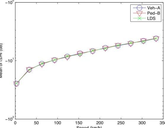
2.9 Mean of |∆/H| versus speed curves. . . 37
3.1 OFDMA frequency description of PUSC mode. . . 39
3.2 Block and serial approaches for ICI equalization. . . 44
3.3 The magnitude of the CFR matrix and cross-sections at selected sub-carriers. . . 46
3.4 This figure shows the percentages of |∆k/Hk| that are larger than 0 dB or smaller than −5 dB at different vehicle speeds. Two channel PDPs, the ITU Pedestrian-B channel and the two-path equal-gain channel, are used. . . 47
3.5 A receiver adopting the PSA framework. . . 48
3.6 A banded CFR matrix with variable bandwidth Q. . . 49
3.7 BER performance comparisons for MAP ICI equalizers under 1024-point FFT, QPSK and ITU Vehicular-A channel model at 500 km/h. The BER curves of the MAP ICI equalizer (solid lines) and the variable Q MAP ICI equalizer (dash lines) essentially overlap. . . 50
3.8 PB ICI equalizer block diagram. . . 53 3.9 SER performance versus |∆k/Hk| at 10, 20 and 30 dB SNR. . . 56
3.10 Empirical probability density functions of α, β and γ for two different channel PDPs: the ITU Pedestrian-B channel and a two-path equal-gain channel. . . 59 3.11 Empirical probability density functions of α, β and γ for the ITU
Pedestrian-B channel at two different vehicle speeds: 350 km/h and 60 km/h. . . . 60 3.12 BER performance comparisons for ICI equalizers under 1024-point FFT,
16-QAM and the ITU Pedestrian-B channel model at 350 km/h and 60 km/h. . . 61 3.13 BER performance comparisons with -20 dB MSE channel estimation
error at 350 km/h. . . 63 3.14 BER with different quantization levels LUT under the ITU Pedestrian-B
channel at 350 and 60 km/h. . . 64 3.15 PER comparison for different Q = 3, 4 and 5 under the ITU Pedestrian-B
channel at 350 km/h. 16-QAM and rate-3/4 CTC are used. . . 66
4.1 Block diagram of the transmitter and receiver of the considered system. Soft-input soft-output (Soft-in-Soft-out) demodulator consists of the ICI equalization such as the feedback canceller [1] and demapper. . . 72 4.2 BER performance with 8-PSK modulation under two-multipath (L = 2)
Rayleigh block fading channels with two different path-gain distribu-tions. The DFT size is 64, P = 2, and a rate-1/2 convolutional code with the generator polynomial [133; 171] (dfree = 10) is adopted. 105
channel realizations are simulated. . . 79 4.3 The eigenvalues are obtained by sampling the convolution of the Doppler
spectrum and the sinc function in frequency domain which can be rec-ognized as the observed Doppler spectrum. The curves show the effect of different window lengths. . . 80 4.4 Comparison of the diversity gain provided by time-varying channels with
three kinds of Doppler power spectral density (PSD): Jakes’ model, uni-form PSD and carrier frequency offset (CFO). The normalized Doppler frequencies 0.01, 0.05 and 0.1 are simulated. The path gains hp(k; l)
for different l are assumed independent. The time-variation of the channel E[hp(k; l)h∗p(m; l
0)] is J
0(2πfd(k − m)T ) · δ(l − l0) for Jakes’
model, sin(2πfd(k − m)T )/(π(k − m)T ) · δ(l − l0) for uniform PSD and
exp(j2πfd(k −m)T )·δ(l −l0) for CFO, where fdis the maximum Doppler
frequency, T is the OFDM sampling time, J0(·) is the zeroth order Bessel
function of the first kind, and δ(·) is the Kronecker delta function. Notice that the considered diversity here is the effective diversity order based on the dominant eigenvalues. . . 82
4.5 BER comparison of the MIMO BICM-OFDM employing CDD, PRD and STBC over doubly-selective fading channels. The DFT size is 64, P = 10, and a rate-1/2 convolutional code with the generator polynomial [133; 171] (dfree = 10) is adopted. Notice that the considered diversity
here is the effective diversity order based on the dominant eigenvalues. The channel is equal-gain two-path at l = 0 and l = 1 and the introduced cyclic delay ∆ is 5. The parameters of PRD are chosen as ε1 = 0.05 and
Chapter 1
Background and Motivation
As mobile data traffic is exploding, many advances in the physical layer of mobile
wireless communications have seen successful deployment in the last two decades. The
data rate of the second generation (2G) digital wireless systems, e.g., Global System for
Mobile Communications (GSM), is about 200 k bits-per-second (bps) and for which
only the voice service is suitable. In the late 1990s, various standards have been
proposed for 3G systems and the data rate is increased up to several Mbps. As wireless
multimedia services become popular, the global data traffic has been doubling each year
during the last few years and the 4G wireless standards such as IEEE’s 802.16 family
and the Long Term Evolution (LTE) by Third-Generation Partnership Project (3GPP)
target to support hundreds of Mbps. To promote these standards, recently, a high
mobility feature has been introduced to enable mobile broadband services at vehicular
speeds up to 350 km/h and even 500 km/h, e.g., in high speed railways. However, the
higher mobility the operating environment has, the larger Doppler frequency spread,
which needs to be coped with, is introduced. In short, wireless communication faces the
ever-increasing demand for higher data rates with more efficient spectrum usage while
maintaining good quality of service in high motion speeds. Two transmission techniques
that are very popular in that regard are bit-interleaved coded modulation (BICM) and
orthogonal frequency-division multiplexing (OFDM). BICM counters fading channels
by spreading codeword bits in time so as to exploit the time diversity available in the
time-varying channel response [2,3], whereas OFDM claims high bandwidth efficiency
and simplicity in receiver design.
Since OFDM has been recognized as an effective technique for high data rate
equiv-alently) [4–6], advanced wireless standards such as worldwide interoperability for
mi-crowave access (WiMAX) and LTE both adopt orthogonal frequency-division multiple
access (OFDMA) as their modulation schemes. High spectral efficiency in such systems
is achieved by tightly squeezing subcarriers into a limited bandwidth [7]. This in turn
implies that, when operating in a high-mobility scenario, for example on a high-speed
vehicle, the channel exhibits fast fading and the signal experiences channel variation
within one OFDMA symbol. This kind of channel is classified as doubly (time and
frequency) selective fading channels. Consequently, the channel frequency response
(CFR) matrix in the transmission model is no longer diagonal, and off-diagonal terms
contribute to severe intercarrier interference (ICI) [8,9]. In other words, the
orthogo-nality between subcarriers is destroyed. As a result, a serious performance degradation
may ensue if ICI is left untreated [10,11].
In this dissertation, we consider the performance of BICM-OFDM systems over
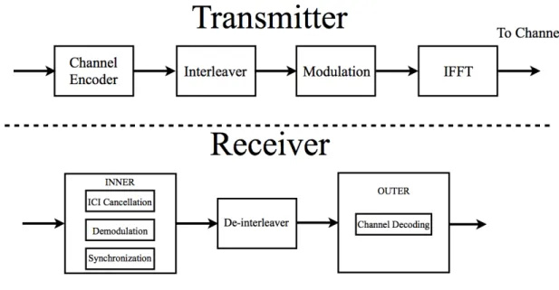
doubly-selective fading channels. As Fig. 1.1 shows, the receiver under consideration
consists of inner and outer parts whereas the inner receiver is mainly for the
com-pensating the impairments caused by the channel and demodulation while the outer
receiver is responsible for channel-decoding. For the inner receiver, we focus on the ICI
problem since it greatly affects the error rate performance. Furthermore, the methods
for dealing with ICI is not limited to BICM-OFDM systems but for all OFDM-based
systems. For the outer receiver, it is interesting to exploit the benefits provides by the
Figure 1.1: Block diagram of a BICM-OFDM system.
1.1
ICI Cancellation for OFDM-Based Systems
One approach to the ICI issue is to cancel it. ICI cancellation for OFDM/OFDMA
systems in doubly selective fading channels has been an active research topic for many
years. Well-known methods abound (please see [8–23] and references therein). Due
to protocol constraints of industrial standards and implementation issues, linear ICI
equalizations in the frequency domain is of particular interest and zero forcing (ZF)
or minimum mean-square error (MMSE) ICI equalizers are proposed in [10,12,13,16].
For these methods, the major computational cost comes from matrix inversion. A
common means to reduce the cost is to approximate the non-diagonal CFR matrix
with a banded matrix in which all but few elements on selected 2Q + 1 diagonals are
set to zero [9,10,12,16,23]. With the banded structure, simpler matrix inversions are
used to calculate MMSE or ZF ICI equalizer coefficients. A rule of thumb in choosing
the bandwidth parameter Q is Q ≥ dfD/∆f e + 1, where fD is the maximum Doppler
frequency and ∆f denotes the subcarrier spacing [9,16]. According to the rule, the
example, in WiMAX Q = 2 for vehicle speeds at 60, 350, and 500 km/h. However, the
BER performance can degrade severely when Q is not large enough. On the other hand,
a large Q may only yield slight performance gain yet induce high complexity. Other
than computational cost, features specified in advanced systems that were derived
from mobile WiMAX (IEEE 802.16e) [7] and LTE can also impose serious difficulties
on engineering development which will be discussed in detail later. Therefore, there
is a strong motivation to seek possible improvement on conventional ICI equalizers to
strike a right balance between performance and implementation complexity.
Based on empirical observations, we found that each subcarrier faces very different
ICI situations and thus, there is no uniform band structure in the CFR matrix, i.e., fixed
Q for every subcarrier. We introduce an useful measure called ICI indicator that can be
used to indicate the relative degree of channel variation (or equivalently the ICI level)
on individual subcarriers [24,25]. With the proposed ICI indicator, appropriate Q’s
can be chosen for each subcarrier that also motivates to use different ICI cancellation
strategies on different subcarriers according to the ICI situation (called per-subcarrier
adaptive (PSA) ICI cancellation framework), say, simple ICI cancellation for
subcar-riers experiencing mild ICI and heavy ICI cancellation for severe ICI. Moreover, as
for the standard’s constraints and implementation readiness, the perturbation-based
(PB) linear ICI equalizers that can be realized as finite-impulse response (FIR) filters
are proposed. A much better trade-off between BER performance and computational
complexity (up to 80 % savings) can be achieved.
We also provide a thorough analysis of the ICI indicator to reveal why it works
and consider some possible applications. Collectively, the probability density
func-tion (PDF) of the ICI indicator provides valuable informafunc-tion, such as the maximum
is only determined by the moving speed in the channel model, and is insensitive to
channel power delay profiles and Doppler power spectra. Therefore, this indicator is
applicable in a wide range of situations of interests.
1.2
BICM-OFDM over Doubly Selective Fading
Chan-nels
Another approach to the ICI issue is, knowing it is a result of channel variation, to
recognize the possibility of using it to gain diversity. Wireless communications face
fading channels and robust data reception is always challenging. One of the most
effective fading countermeasures is using the diversity techniques to exploit available
diversity gain offered by the channel. By introducing a bit interleaving between the
channel encoder and mapper, BICM was first proposed by Zehavi in [26] and then
comprehensively investigated by Caire et al. [2]. A further development, BICM with
iterative decoding (BICM-ID), is proposed by Li et al. [3]. The diversity order of
BICM in flat fading channels is found to be the minimum number of distinct bits in
two different code sequences and can be very high in a properly design BICM system.
A lot of literatures about BICM deal with the flat fading channels; therefore, only
temporal diversity is utilized. For the purpose to exploit frequency diversity as well,
the combination of OFDM and BICM, called BICM-OFDM, over frequency selective
fading channels is an attractive option. It is shown to achieve the maximum diversity
order inherent in such channel [27]. Since many existing and future wireless standards
employ bit-level interleaver and channel coding, e.g., WiFi, DVB, WiMAX, LTE and
Doubly selective fading channels in many situations have been viewed as the cause
of severe channel impairments such as ICI, it is also considered as a potential source of
time and frequency diversity which may enhance the system performance. Compared
to the performance with quasi-static channels, utilizing the ICI terms at the receiver
may actually improve the error rate and simulation results also reveal that the
per-formance gain comes from increasing diversity [9,12,28]. Pioneering work by Ma and
Giannakis [29] considers the maximum diversity order over doubly selective channels
for general block transmission systems without forward error correction (FEC). Recent
papers start investigating time diversity for coded OFDM systems. Huang and
oth-ers [1,18] reported that, in simulations the performance of BICM-OFDM systems is
improved when the channel is fast fading. In [27], the diversity order of BICM-OFDM
systems in frequency selective fading channels is analyzed. For BICM-OFDM systems,
a theoretical analysis of the diversity order over doubly selectively fading channels has
not appeared in the literature. It motivates us to provide such analysis and the
maxi-mum diversity order of BICM-OFDM over doubly selective fading channels is derived.
First, we derive the asymptotic diversity order of BICM-OFDM systems by
study-ing the role of correlation in rank analysis of the typical derivation of diversity order.
The results also show that BICM-OFDM achieves the maximum diversity order given
in [29]. Second, the effect of significant eigenvalues of the channel correlation matrix
and the diversity order in realistic situations with moderate SNRs are examined by
studying the channel correlation function and its Fourier dual. Finally, our analysis
framework is extended to multiple input multiple output (MIMO) cases while
incorpo-rating more diversity techniques, such as cyclic delay diversity (CDD) and phase-roll
diversity (PRD) [30]. This MIMO extension can also be applied in a distributed
1.3
Thesis Organization
This dissertation is organized as follows. In Chapter 2, we give an extensive review of
the doubly selective fading channels including the statistical characterization, discrete
time model and generating approaches for computer simulations. With the
develop-ment of system model of OFDM systems over doubly selective fading channels, a novel
ICI indicator is introduced and the statistical analysis as well as possible applications
of the ICI indicator are given. Chapter 3 discusses the ICI cancellation and introduces
the PSA framework. The PSA PB-ZF and PB-MMSE ICI equalizers that consider the
standard constraints and are suitable for implementation are presented. In Chapter 4,
the asymptotic and practical diversity orders of BICM-OFDM systems over
doubly-selective fading channels are theoretically analyzed. The analysis can be extend to
MIMO cases and two techniques, CDD and PRD, are discussed. Finally, we consider
Chapter 2
Doubly Selective Fading Channels
Wireless communication often encounters environments with rich multipaths because of
the atmospheric scattering and refraction, or reflections of surrounding objects.
Trav-eling through these paths, the signals arrived at the receiver with random delays and
attenuations will be added constructively or destructively and result in envelope
fluc-tuations significantly, which is referred to fading. Furthermore, in high data rate
wide-band systems, e.g., OFDM, the wide-bandwidth of the transmitted signal is larger than the
coherence bandwidth of the fading channel, giving rise to frequency-selectivity of fading
channels. It becomes clear that emerging mobile applications will experience channel
variations within one symbol time where the channel is said to be time-selective. This
is mainly due to the changing atmospheric conditions and relative movements between
transmitters and receivers. Consequently, the wireless channel of mobile
communi-cations is characterized as a time- and frequency-selective (or doubly-selective) fading
channel. As these selectivities affect the system performance critically, the
understand-ing and modelunderstand-ing of doubly-selective fadunderstand-ing channels are important tasks for devisunderstand-ing
countermeasures.
A precise mathematical description of fading channels, i.e., the physical modeling
based on electromagnetic radiation [32], for practical scenarios is either unknown or
too complex to be tractable. However, considerable efforts have been devoted to the
statistical modeling. Moreover, statistical descriptions could provide insights in many
typical issues, e.g., the proper packet duration to avoid fades, the relative severity of
necessary interleaving depth for time diversity, expected BER, etc..
In this chapter, we first consider the statistical characterization of doubly-selective
fading channels. Then, the discrete-time channel model will be developed and channel
simulators for computer simulations will be introduced. As OFDM has become the de
facto transmission scheme in modern wireless communications, we consider the system
model for OFDM over doubly-selective fading channels where ICI exists. Based on
empirical observations, a measure called the ICI indicator was introduced to indicate
the ICI level as well as to estimate the maximum Doppler frequency on each
subcar-rier. We also provide a thorough analysis of the ICI indicator to reveal why it works.
Collectively, its PDF also provides valuable information on, for example, the maximum
Doppler spread. Some applications of the ICI indicator are given.
2.1
Baseband Equivalent Representation and
Sta-tistical Characterization
Assume there exist multiple propagation paths, αn(t) is the attenuation factor for the
signal received on the n-th path, and τn(t) is the propagation delay of the n-th path.
The bandpass received signal through discrete multipath channels in the absence of
noise can be expressed in the form
y(t) =X
n
αn(t)x(t − τn(t)) (2.1)
where x(t) is the bandpass transmit signal.
Using the complex envelope and expressing x(t) as Re[xbb(t)ej2πfct] where xbb(t) is
the baseband equivalent transmit signal and fc is the central carrier frequency, we can
at baseband. Equation (2.1) can be re-written as
y(t) = Re[{X
n
αn(t)e−j2πfcτn(t)xbb(t − τn(t))}ej2πfct]. (2.2)
From the above expression it is straightforward to write the baseband equivalent (or
lowpass equivalent) signal as
ybb(t) =
X
n
αn(t)e−j2πfcτn(t)xbb(t − τn(t)). (2.3)
By transmitting a conceptually ideal impulse, the complex baseband equivalent
time-varying channel impulse response (CIR) is obtained as
c(t; τ ) =X n αn(t)e−j2πfcτn(t)δ(t − τn(t)) =X n ˜ αn(t; τ )δ(t − τn(t)) (2.4)
where δ(·) denotes the Dirac delta function.
For another type of channel model, the diffuse multipath channel, the signal is
composed of a continuum of unresolvable components and is expressed in the integral
form
y(t) = Z ∞
−∞
α(t; τ )x(t − τ )dτ (2.5)
where α(t; τ ) denotes the attenuation of the signal at delay τ and at time instant t.
Following the similar procedures as in the case of discrete multipath channels, the CIR
can be expressed by
c(t; τ ) = α(t; τ )e−j2πfcτ. (2.6)
In Equation (2.4), the channel fading is described by time variations in the
mag-nitudes and phases of c(t; τ ). These variations appear to be random and usually are
treated as random processes. If there are numerous propagation paths, which usually
Gaussian random process by the central limit theorem. When the CIR is zero-mean,
the envelope r = |c(t; τ )| is Rayleigh-distributed that has the form [33]
fR(r|σ2) =
r σ2e
−r2/(2σ2)
, r ≥ 0 (2.7)
and it is called the Rayleigh fading channel. This kind of simplification often applies to
the non-light-of-sight (NLOS) case. When there is a direct-link between the transmitter
and the receiver, i.e., the LOS case, the CIR cannot be modeled as zero-mean, and the
channel is often modeled by Ricean fading following the PDF [33]
fR(r|ν, σ2) = r σ2e −(r2+ν2)/(2σ2) I0( rν σ2), r ≥ 0 (2.8)
where I0(·) is the zero-th order modified Bessel function of the first kind. When ν = 0,
which means the power of the LOS path is zero, the distribution reduces to a Rayleigh
distribution.
As the basic Rayleigh/Ricean model gives the PDF of the channel envelope, we
now consider the question of how fast the signal fades in time and frequency. To answer
the question, we need further characterize the CIR by its autocorrelation function and
power spectral density (PSD); together they form a Fourier transform pair [33].
2.1.1
Channel Autocorrelation Functions and Power Spectra
Autocorrelation Functions
We assume c(t; τ ) is wide-sense-stationary (WSS) and define the autocorrelation
func-tion of c(t; τ ) as
Rc(∆t; τ1, τ2) = E[c(t; τ1)c∗(t + ∆t; τ2)]. (2.9)
In most cases, the attenuation and phase shift at the delay τ1 path is uncorrelated with
(2.9) can be decoupled into
Rc(∆t; τ1, τ2) = Rc(∆t; τ1)δ(τ2− τ1). (2.10)
Notice that Rc(0; τ ) , Rc(τ ) is called the power delay profile (PDP); the range of τ
within which Rc(τ ) is non-zero is termed the maximum delay spread of the channel
and is denoted as Tm.
PDP describes the average received power as a function of delay and is one of the
most important parameters for channel modeling. We will see later that many
indus-trial standards specify PDPs in their testing environments. PDP can be measured by
probing the channel with a wideband radio-frequency (RF) waveform that is generated
by modulating a high-rate pseudo-noise (PN) sequence. By cross correlating the
re-ceiver output against delayed versions of the PN sequence and measuring the average
value of the correlator output, one can obtain the power versus delay profile. Just like
there are may equally valid definitions of bandwidth, other useful measurements of the
delay spread are possible. One of them is the root-mean-square (RMS) delay spread,
which is defined by TRMS = s R τ2R c(τ )dτ R Rc(τ )dτ − (R τ Rc(τ )dτ R Rc(τ )dτ )2. (2.11)
Now consider channel characterizations in the frequency domain. By taking the
Fourier transform of c(t; τ ) w.r.t. the variable τ , the time-variant channel frequency
response is
C(t; f ) = Z ∞
−∞
c(t; τ )e−j2πf τdτ. (2.12)
Similarly, we can define the autocorrelation function of C(t; f ) as
Relating (2.13) to (2.10), it can be shown that RC(∆t; f1, f2) = Z ∞ −∞ Rc(∆t; τ1)e−j2π∆f τ1dτ1 , RC(∆t; ∆f ) (2.14)
where ∆f = f2 − f1. Equation (2.14) describes the autocorrelation function in the
frequency variable. Moreover, the range of ∆f within which the components of RC(∆f )
are highly correlated is defined as the coherence bandwidth of the channel and denoted
as (∆f )c. As Rc(∆t; τ1) and RC(∆t; ∆f ) form a Fourier transform pair, a very rough
relation is that the coherence bandwidth is reciprocally proportional to the maximum
delay spread [33]
(∆f )c≈
1 Tm
. (2.15)
If the signal bandwidth is large compared to the channel’s coherence bandwidth, the
signal will be distorted and the channel is called frequency-selective. This is equivalent
to the case where the delay spread is larger than the symbol time, which is also termed
time-dispersion because transmitting an ideal impulse through the channel will yield a
receive signal with several delayed pulses. In this case, the interference among different
symbols occur and called inter-symbol interference (ISI).
Power Spectral Density
Now, we consider the time variations of the channel and investigate the Fourier
trans-form pair
SC(λ; ∆f ) =
Z ∞
−∞
RC(∆t; ∆f )e−j2πλ∆td∆t. (2.16)
If ∆f is set to 0, SC(λ) is called the channel’s Doppler PSD and λ represents the
Doppler frequency. The range of λ within which SC(λ) is non-zero is termed the
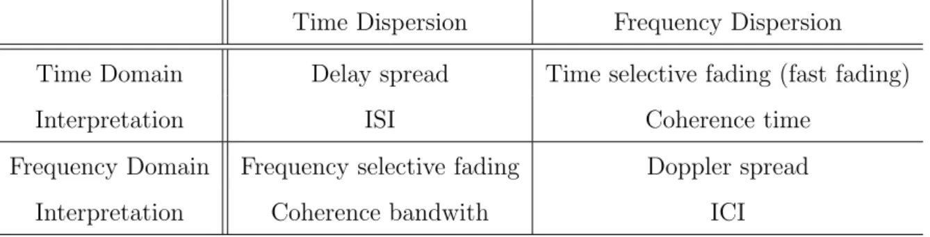
Table 2.1: Time and Frequency Dispersion
Time Dispersion Frequency Dispersion Time Domain Delay spread Time selective fading (fast fading)
Interpretation ISI Coherence time
Frequency Domain Frequency selective fading Doppler spread
Interpretation Coherence bandwith ICI
frequency can be roughly calculated by
fD =
vfc
c (2.17)
with v being the mobile speed and c the speed of light. Similarly, the range of ∆t
within which the components of RC(∆t) are highly correlated is defined as the channel’s
coherence time and is denoted as (∆t)c. Again, because they form a Fourier transform
pair, the maximum Doppler spread and the coherence time are reciprocally related via
(∆t)c≈
1 fD
. (2.18)
Similarly, if the signal duration is large compared to the channel’s coherence time,
the channel is called time-selective. This is equivalent to the case where the Doppler
spread is large enough, and a pure-tone transmit signal passing through the channel
will yield a receive signal with several frequency components; we call this phenomenon
frequency-dispersion. The terminologies and their relationships are summarized in the
Table 2.1.
To relate the parameters τ , λ, ∆f , and ∆t, we define the scattering function of
the channel
Ssc(λ; τ ) =
Z ∞
−∞
which is the double Fourier transform of RC(∆t; ∆f ).
Jakes’ model is widely adopted to describe the time variation of the mobile radio
channels with the the corresponding autocorrelation function
RC(∆t) = J0(2πfD∆t) (2.20)
where J0(·) is the zero-th order Bessel function of the first kind. The Dopper PSD is
obtained by Fourier transform, that is
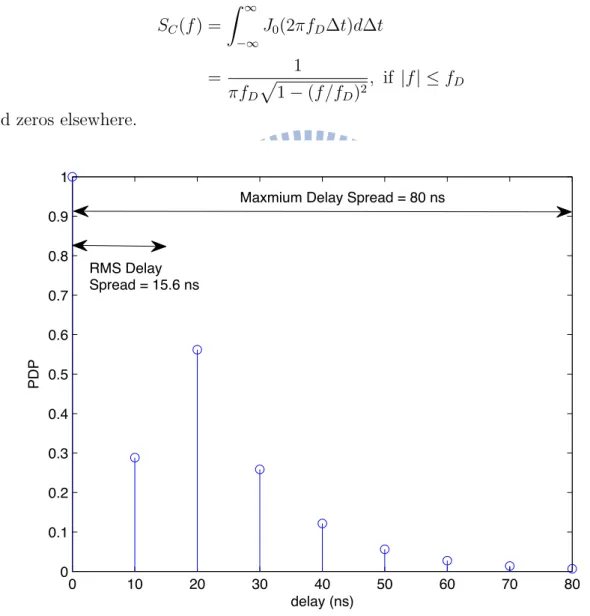
SC(f ) = Z ∞ −∞ J0(2πfD∆t)d∆t = 1 πfDp1 − (f/fD)2 , if |f | ≤ fD (2.21)
and zeros elsewhere.
0 10 20 30 40 50 60 70 80 0 0.1 0.2 0.3 0.4 0.5 0.6 0.7 0.8 0.9 1 delay (ns) PDP
Maxmium Delay Spread = 80 ns
RMS Delay Spread = 15.6 ns
Figure 2.1: PDP of IEEE 802.11n channel model B.
Here we give some examples of the statistical channel parameters in practical
indoor, there are five channel models proposed by the IEEE 802.11 a/n standard [34]
where the RMS delay spreads are about 0 ns to 150 ns depending on the scenarios,
and the Doppler power spectrum is Bell-shaped, specified by
SC(f ) =
1 1 + A(ff
D)
2. (2.22)
Fig. 2.1 shows the PDP of the IEEE 802.11n channel B whose the maximum delay
spread is 80 ns and the RMS delay spread is 15.6 ns. According to (2.15), the
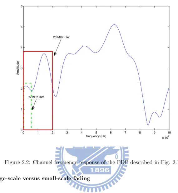
co-herence bandwidth is around 12.5 MHz. The channel frequency response is shown
in Fig. 2.2 and it can be seen that the signal with 20 MHz bandwidth experience
frequency-selectivity while the CFR varies slow within 5 MHz and thus the channel of
the signal with 5 MHz bandwidth can be considered as flat-fading. However, since the
application is in indoor, the mobility is very small and the channel varies very slowly
so we demonstrate the Doppler effect in the following example.
For the wireless Metropolitan Area Network (MAN), e.g., IEEE 802.16e, the
Inter-national Telecommunication Union (ITU) channel models are adopted where the RMS
delay spreads for outdoor scenarios are around 2 us to 20 us, much longer than that of
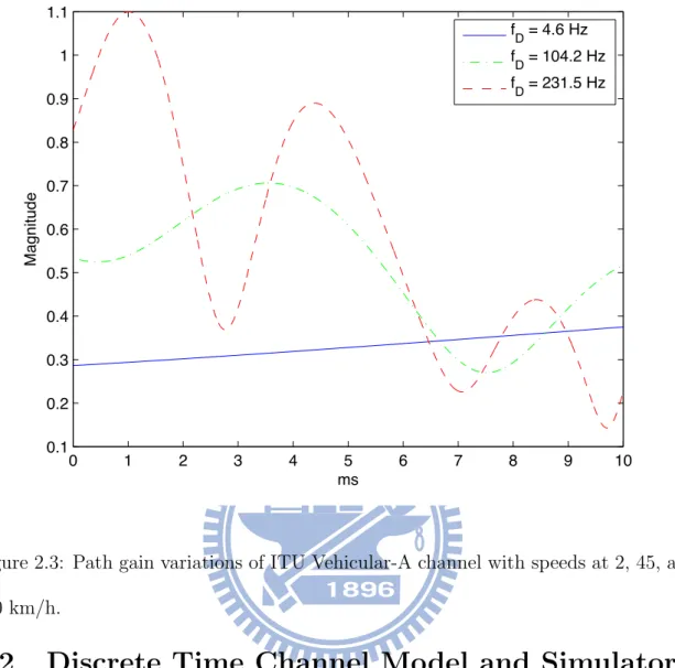
WLAN scenarios. The Jakes’ U-shape Doppler spectrum is assumed and the typical
maximum Doppler spreads at 2.5 GHz carrier frequency are 4.6, 104.2, and 231.5 Hz
corresponding to the speed of 2, 45, and 100 km/h, respectively. The corresponding
coherence time is 200, 10, and 4 ms, respectively. Fig. 2.3 shows the path gain
varia-tions of ITU Vehicular-A channel and it can be seen that higher speeds result in faster
channel variations. In IEEE 802.16e, the symbol duration is around 100 µs so that
even at 100 km/h the channel still can be considered as linearly time-varying within
0 1 2 3 4 5 6 7 8 9 10 x 107 0 1 2 3 4 5 6 frequency (Hz) Amplitude 5 MHz BW 20 MHz BW
Figure 2.2: Channel frequency response of the PDP described in Fig. 2.1.
Large-scale versus small-scale fading
It is worthwhile to mention that channel fading can also be categorized into large-scale
and scale fading [32]. While we have discussed the causes and effects of
small-scale fading in the above, the large-small-scale fading is caused by propagation loss over long
distance and by shadowing due to obscuring objects that attenuate the received signal
strength. Since large-scale fading varies much slower compared to small-scale fading
and the induced issues are more related to cell planning and receivers’ sensitivity, in
0 1 2 3 4 5 6 7 8 9 10 0.1 0.2 0.3 0.4 0.5 0.6 0.7 0.8 0.9 1 1.1 ms Magnitude f D = 4.6 Hz f D = 104.2 Hz f D = 231.5 Hz
Figure 2.3: Path gain variations of ITU Vehicular-A channel with speeds at 2, 45, and
100 km/h.
2.2
Discrete Time Channel Model and Simulators
It has been shown that both PDP and Doppler PSD are effective tools to characterize
wireless channels, we now consider the problem of how to efficiently generate channels
for computer simulations. We focus on Rayleigh fading since the Ricean model can be
obtained from the Rayleigh model by adding a non-zero mean.
2.2.1
Discrete Time Model
For most time the input-output relationship can be modeled as a linear time-varying
the intensive computational complexity due to very high oversampling. It has been
shown that using discrete time representation realized by a tapped delay line model
with time-variant tap gains is usually good enough for simulation purposes.
Let pT(t) and pR(t) be the time-invariant impulse response of the transmit filter
and the receive filter, respectively, and both are normalized with unit energy. At the
receiver, the resulting channel will have the combined impulse response as
h(t; τ ) = pR(τ ) c(t; τ ) pT(τ ) (2.23)
where a(τ ) b(t; τ ) = R b(t; τ0)a(τ − τ0)dτ0 denotes the convolution operation. We consider typical digital communication where the transmit sequence s(l) consists of
complex symbols with the symbol time equals to Tsym. By replacing (2.4) with (2.23)
and using (2.3), the baseband equivalent received signal y(t) can be expressed by
y(t) =X
l
x(l)h(t; t − lTsym) (2.24)
where the subscript bb in (2.3) is omitted for brevity unless stated otherwise since
we are concerned with the baseband equivalent model throughout most part of this
dissertation.
The sampled version of y(t) with the sampling period Ts is given by
y(kTs) =
X
l
x(l)h(kTs; kTs− lγTs) (2.25)
where γ is an integer oversampling factor and Ts = Tsym/γ. For considering RF- or
analog-related effects, it may require oversampling, e.g., γ = 2, 4, .... If oversampling is
used, the data sequence {x(k)} should also be oversampled by inserting (γ − 1) zeros
between each symbol x(k). It can be shown that the symbol-spaced model contains
sufficient statistics for data detection if the transmit and receiver filters are carefully
chosen, i.e., fulfilling the Nyquist condition. Consequently, we consider the the case
2.2.2
Channel Simulators
As the discrete time channel model in Equation (2.25) acts as an FIR time-varying
filter, the problem is transformed to generating the tap gains for simulations. We
consider two well-known methods: the first is to generate and combine several complex
exponentials, and thus is properly termed sum-of-sinusoidal; the second is to generate
a Gaussian random sequence and passing the sequence through an FIR filter with the
transfer function designated to be the square-root of the required Doppler PSD.
Simulation Methods I: Sum-of-sinusoidals
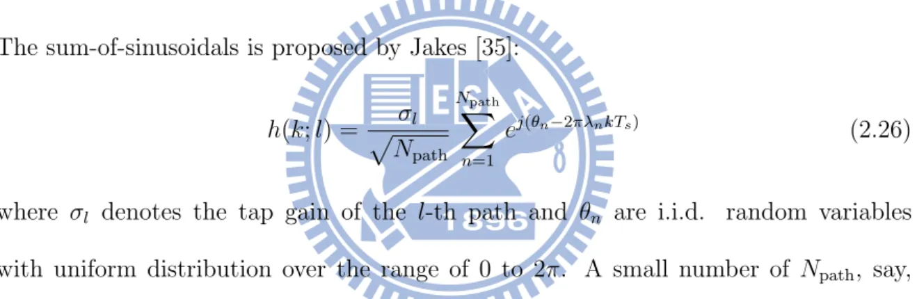
The sum-of-sinusoidals is proposed by Jakes [35]:
h(k; l) = σl pNpath Npath X n=1 ej(θn−2πλnkTs) (2.26)
where σl denotes the tap gain of the l-th path and θn are i.i.d. random variables
with uniform distribution over the range of 0 to 2π. A small number of Npath, say,
Npath = 10, will approximate Rayleigh fading quite accurately. The block diagram of
the channel tap generation process is shown in Fig. 2.4.
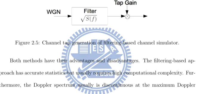
Simulation Methods II: Filtering
Another approach to simulate the tap gains with desired PDP and Doppler spectrum
is [36,37]: first generate a complex white Gaussian random sequence; second, input the
generated sequence to an FIR filter with the square root of the desired Doppler PSD
as its transfer function; finally, properly scale the corresponding filter tap to follow the
desired PDP. The block diagram of the channel tap generation process is shown in Fig.
2.5.
Figure 2.5: Channel tap generation of filtering-based channel simulator.
Both methods have their advantages and disadvantages. The filtering-based
ap-proach has accurate statistics but usually requires high computational complexity.
Fur-thermore, the Doppler spectrum usually is discontinuous at the maximum Doppler
frequencies and it makes the corresponding FIR filter to be very long. The statistics
associated with the sum-of-sinusoidal approach may not be what we expect and some
techniques have been proposed to improve the accuracy [38–40].
2.3
OFDM Systems over Doubly-Selective Fading
Channels
OFDM is a promising transmission technique to achieve high data rates over wireless
mobile channels. Besides bandwidth efficiency, OFDM offers many advantages over
spread, all-digital-FFT implementation, the possibility of adaptive channel allocation
and adaptive modulation of the subcarriers for maximizing the capacity [41]. Thanks
to cyclic prefix (CP), the ISI can be avoided, and the channel effect can easily be
com-pensated by applying one-tap frequency domain equalizers since the frequency selective
fading channel is transformed into parallel flat fading channels. However, if there
ex-ists channel variations within one OFDM symbol will introduce interferences among
subcarriers, called ICI. OFDM is vulnerable to ICI due to tightly spacing between
subcarriers.
Consider the baseband equivalent OFDM system model with N subcarriers. By
doing N -point IDFT of the data sequence of the OFDM symbol, {S(m)}, the
time-domain transmitted signal x(k) at the k-th time instant can be written as
x(k) = 1 N N −1 X m=0 S(m)ej2πmkN , k = 0, 1, · · · , N − 1. (2.27)
Assume a CP with length of NCP longer than the maximum delay spread of the channel,
denoted as L; the total length of a transmitted OFDM symbol is NS = N + NCP. Let
h(k; l) represent the l-th delay path of the time-varying dispersive channel impulse
response at the k-th sampling instant. The channel path {h(k; l)} is assumed to follow
the WSSUS model, i.e., E[h(k; l)h∗(k; l+l0)] = σ2
lξl0 where ξl0denotes the 1-D Kronecker
delta and σ2
l is the average power of the l-th path. Assuming CP removal and perfect
synchronization, the sampled baseband equivalent received signal y(k) of the OFDM
symbol can be expressed as [9,10]
y(k) =
L−1
X
l=0
h(k; l)x(k − l) + n(k), 0 ≤ k ≤ N − 1 (2.28)
where n(k) is the additive white Gaussian noise.
re-ceived signal on the i-th subcarrier is R(i) = N −1 X k=0 y(k)e−j2πkiN = N −1 X k=0 ( L−1 X l=0 h(k; l)x(k − l) + n(k))e−j2πkiN = N −1 X k=0 ( L−1 X l=0 h(k; l)(1 N N −1 X m=0 S(m)ej2πm(k−l)N ) + n(k))e −j2πki N = N −1 X m=0 S(m)Hi,m+ Z(i) (2.29) where Hi,m = 1 N X k H(m; k)e−j2πk(i−m)N (2.30) and H(m; k) =X l h(k; l)e−j2πlmN . (2.31)
Note that H(m; k) can be interpreted as the CFR on the m-th subcarrier at the k-th
time instant. The ICI on the i-th subcarrier which is caused by the signal on the m-th
subcarrier comes through the ICI channel Hi,m.
Assume that the time variation of CIR is linear within one OFDM symbol [13,15].
It is a reasonable assumption in most practical cases when the normalized Doppler
frequency (normalized to subcarrier spacing) is smaller than 0.1, which corresponds to
500 km/h in WiMAX standard. The CIR of the p-th OFDM symbol can be written as
h(pNS− N + k; l) = h(pNS − N − 1 2 ; l) + k − N −1 2 NS δ(pNS; l) (2.32)
where NS denotes the length of CP plus N . h(pNS−N −12 ; l) represents the center point
of the p-th OFDM symbol and δ(pNS; l) is the slope of the l-th channel path at the
p-th OFDM symbol. Note that with the linear variation assumption the channel at the
center point is also the averaged channel in one OFDM symbol.
form as
y = HtFHx + n (2.33)
where y = [y(0), y(1), · · · , y(N − 1)]T, [H
t]k,l = h(pNS − N + k; (k − l) mod N )
denotes the CIR matrix, [F]m,n = (1/
√
N )e−j2πmn/N is the N -point DFT matrix, s = [S(0), S(1), · · · , S(N − 1)]T, and n = [n(0), n(1), · · · , n(N − 1)]T.
Using (2.32), the CIR matrix in (2.33) can be decomposed as
Ht = Mt+ ψDt (2.34)
where [Mt]k,l = h(pNS−N −12 ; (k − l) mod N ) and [Dt]k,l = δ(pNS; (k − l) mod N ) for
k, l = 0, 1, . . . , N −1. Mtand Dtboth are circulant matrices. The matrix ψ is diagonal
and defined as ψ = N1 Sdiag([− N −1 2 , − N −1 2 + 1, . . . , N −1 2 ] T). Note that h(pN S− N −12 ; l)
and δ(pNS; l) are assumed to be zero when l ≤ 0 or l ≥ L − 1.
Substituting (2.34) into (2.33) and applying DFT matrix to y, the received signal
r = [R(0), R(1), · · · , R(N − 1)]T in the frequency domain is given by r = Fy = FMtFH | {z } ≡Havg s + FψFH | {z } ≡G FDtFH | {z } ≡∆ s + Fn = Havgs + G∆s | {z } ICI +z (2.35)
where Havg+G∆ is the CFR matrix and z is the AWGN in the frequency domain. The
term G∆s represents ICI which is determined by ∆ and a fixed matrix G where ∆
is DFT of the slope of the CIR, Dt. Note that since Mt and Dt are circulant matrix,
Consequently, the CFR matrix can be decomposed as Hf = Havg+ G∆ = H0 0 · · · 0 0 H1 ... .. . . .. 0 0 · · · 0 HN −1 + 0 G−1 · · · G−(N −1) G1 0 ... .. . . .. G−1 GN −1 · · · G1 0 ∆0 0 · · · 0 0 ∆1 ... .. . . .. 0 0 · · · 0 ∆N −1 . (2.36)
Now, a tiny yet crucial rearrangement of this well-known ICI signal model is in
order. By multiplying both sides of (2.35) by the diagonal matrix (∆H−1avg), we can rearrange (2.35) into: (∆H−1avg)r | {z } ˜r = [IN + (∆H−1avg)G] | {z } ˜ H (∆s) | {z } ˜s + (∆H−1avg)z | {z } ˜z (2.37)
where IN denotes the N ×N identity matrix, and ˜s acts as the transmitted signal, ˜r the
received signal and (∆H−1avg)G as the ICI channel. Note that in (2.35), ∆ multiplies G from the right; it follows that the column vectors of the CFR matrix are weighted
by different ∆k. This model registers how the signal on each subcarrier is spread
over and comes to interfere other subcarriers. Different weights represent different
spreading effects for each subcarrier. In (2.37), however, G is multiplied by the diagonal
matrix (∆H−1avg) from the left; this time, row vectors of the CFR matrix are weighted with a different (∆k/Hk). This model registers how a subcarrier is interfered by its
neighboring subcarriers. Different weights indicates different ICI levels experienced by
2.4
ICI Indicator
The ICI model in (2.35) and (2.37) provides more insights when it is examined at the
subcarrier-level granularity. There is no uniform band structure in the CFR matrix
since each subcarrier faces very different ICI situations. In (2.37), (∆H−1avg)G represents the ICI channel; this motivates us to propose the metric |∆k/Hk| to indicate the ICI
level on each subcarrier. From (2.37), define the Signal-to-Interference Channel power
Ratio (SICR) on the k-th subcarrier as
SICRk =
| ˜Hk,k|2
PN −1
m=0,m6=k| ˜Hk,m|2
, (2.38)
which can be further approximated to
SICRk≈ N2 4π2N2 s ∆k Hk 2 2 N/2−1 X i=1 1 |i|2 −1 ≈ 12N 2 S N2|∆ k/Hk|2 (2.39) where |Gi| ≈ 2πNN S 1 |i| and P∞ i=1 1 |i|2 = π2
6 are used. Note that the SICR is inversely
proportional to |∆k/Hk|2. For example, if a subcarrier suffers little ICI, the SICR
(≥ 22 dB) will be quite high and |∆k/Hk| (≤ −5 dB) is low. On the other hand, when
deep fading occurs at some subcarrier, |∆k/Hk| becomes large (≥ 0 dB) and SICR
(≤ 12 dB) is low, and the demodulated symbol tends to be wrong due to severe ICI.
To better utilize |∆k/Hk| as the ICI indicator, its statistical properties are
inves-tigated. Assuming Rayleigh fading channels, δ(nN s; l) and h(nNS− N −12 ; l), the CIR
slope and the averaged CIR, are zero-mean circular complex Gaussian random variables
(RVs) with variances σ2
δ(nN s;l) and σ 2
h(nNS−N −12 ;l)
. It follows that ∆kand Hkare also
zero-mean circular complex Gaussian RVs with variances P
lσ 2 δ(nN s;l) and P lσ 2 h(nNS−N −12 ;l)
variance σ2, the PDF of A is given by pA(a) = 1 πσ2 exp{− |a|2 σ2 }. (2.40)
It is well known that the magnitude of A, B = |A|, follows a Rayleigh distribution
with parameter σ2/2 as pB(b) = b σ2/2exp{− b2 σ2}, if b ≥ 0, (2.41) and pB(b) = 0 elsewhere.
To simplify the derivation, we further assume ∆k and Hk are uncorrelated, on the
grounds that ∆k is caused by the mobility of scatterers while Hk is mainly determined
by the reflection property of scatterers. This property is also shown in [13] in which the
zeroth-order and the first-order derivative in the power series expansion of the channel
correspond to our Hk and ∆k. Define X , 10log10(|∆k|) and Y , 10log10(|Hk|). Since
|∆k| and |Hk| are Rayleigh RVs with parameters 12 Plσδ(nN s;l)2 and 12Plσh(nN2
S−N −12 ;l),
X and Y follow the Log-Rayleigh distribution with the PDF [42], which can be derived
from (2.41) by using the technique of function of RV, is given by
p(ϕ|η2) = (e
ϕ/c)2
cη2 exp (−
(eϕ/c)2
2η2 ) (2.42)
where the constant c = 10 log10(e) and η2 is the so-called localization parameter that
equals to 12P lσ2δ(nN s;l) for X and 1 2 P lσh(nN2 S−N −1 2 ;l)
for Y . Since 10log10(|∆k|
|Hk|) =
10log10(|∆k|) − 10log10(|Hk|), the PDF of 10log10( |∆k|
|Hk|) can be obtained as
p(ω) = Z ∞
−∞
pX(ω + y|ηX2)pY(−y|η2Y)dy, (2.43)
η2
X and ηY2 being the localization parameters of X and Y . Using the property that the
mean of Log-Rayleigh PDF is 10 log10(η2) + c0 where c0 = 2c(ln 2 +R0+∞ln v exp(−v)dv) is a constant and the variance is c224π2 [42], it follows that the PDF of 10log10(|∆k|
depends on the ratio between P lσ 2 δ(nN s;l) and P lσ 2 h(nNS−N −12 ;l). Intuitively, channel
variation is caused by mobility rather than depends on the channel PDP. We expect
the ratio to be insensitive to PDPs. In this case, the PDF of the ICI indicator will be
consistent over a wide range of channels with different PDPs.
−30 −25 −20 −15 −10 −5 0 5 10 15 0.02 0.04 0.06 0.08 0.1 0.12 0.14 | k/Hk| (dB) PDF Theoretical Vehicular−A Two−path 60 km/h 120 km/h 350 km/h
Figure 2.6: Probability density functions (solid lines) and two histograms (dash lines for
the ITU Vehicular-A channel and dots for two-path equal gain channel) of 10log10(|∆k
Hk|)
for moving speeds at 60, 120 and 350 km/h. Bell-shape Doppler power spectrum and
uncorrelated scattering are used.
Simulation is conducted to verify the theoretical result, using the WiMAX
stan-dard with 10 MHz bandwidth, 2.5 GHz central frequency, 1024 subcarriers. Two
channel models with very different PDPs, the ITU Vehicular-A and a two-path equal
gain channel, are used. Fig. 2.6 shows the theoretical PDF and the histogram of
10log10(|∆k
theo-retical analysis of PDF is valid. Recall that larger |∆k/Hk| means higher ICI level.
As the moving speed gets higher, more subcarriers experience severe ICI; yet even at
350 km/h, there still is a major portion of subcarriers experiencing mild ICI. It is also
observed from Fig. 2.6 that the distribution of |∆k/Hk| remains essentially the same
when two quite different PDPs are used. The PDF can be used in evaluating the
ben-efit of reducing complexity by adapting ICI equalizers according to the ICI indicator.
Details can be seen in Chapter 3.
−15 −10 −5 0 5 10 0 0.02 0.04 0.06 0.08 0.1 0.12 | k/Hk| (dB) PDF Theoretical Flat Doppler PSD Correlated scattering
Figure 2.7: Probability density functions (solid lines) and two histograms (dash lines
for the flat Doppler spectrum and dots for the correlated scattering with correlation
0.7 between paths) of 10log10(|∆k
Hk|) for moving speed at 350 km/h. Two-path equal
gain channel is used.
Other factors that may affect the PDF are also investigated. In Fig. 2.7, the
seen, the PDF is also quite insensitive to the Doppler spectrum shape. In contrast, the
correlation existing among channel paths can change the PDF. However, the overall
trend is still that the PDF’s center becomes larger when the moving speed gets larger,
so does the maximum Doppler spread. Therefore, the ICI indicator can still offer useful
information on channel variations.
In practice, the ICI indicator is obtained as the ratio between the estimates of
∆k and Hk. An estimation method that uses consecutive OFDM symbols is provided
in [15]. Here, with the goal of keeping complexity low, a simpler method is used.
Instead of estimating the complete ICI model as in [15], we use the estimate of the
averaged CFR, ˆHk, which is always needed for signal demodulation. The estimate of
∆k is simply obtained as the difference between ˆHk of adjacent OFDM symbols due to
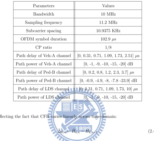
the fact that CFR varies linearly across time-domain:
ˆ
∆k,n= ˆHk,n− ˆHk,n−1
where second index in the subscript denotes the symbol index. Though the estimate
is not very accurate, the degradation in simulated BER performance is insignificant.
Channel estimation for time-varying channels may also be used [8,10–13], but we
re-gard this as unnecessary in the current setting. To support higher Doppler spreads in
the future, better channel estimation will be needed and advanced channel estimation
techniques can be found in [43–47] and extended for MIMO channels in [48,49].
Fur-thermore, to jointly estimate the channel and other synchronization parameters has
2.5
Applications of ICI Indicator
In a vehicular network, a variety of communication types exist: vehicle-to-vehicle,
vehicle-to-station, and vehicle-as-relay, etc. Together with the vastly different velocities
at which each vehicle in the network moves, a very complicated landscape of relative
velocities may exist. Due to the fact that the fading rate experienced at a receiver highly
depends on the relative speed between the receiver and the transmitter, it becomes clear
that a very diverse and dynamic fading environment is a reality that vehicular networks
need to face on a regular basis. It is also well known that the information of fading
rate can be utilized to adapt many communication subsystems to improve the overall
performance. Therefore, the ability to make a timely estimation of the fading rate on
each link can be a great asset to the nodes operating in a vehicular network.
The estimation of fading rate can not be always accomplished by deriving from
the speed information obtained by global positioning system (GPS). For example, in
a vehicle-to-vehicle link, the relative speed cannot be derived from GPS information
before the link is established; however, the fading rate information may be valuable in
establishing such a link. For another example, the fading rate may be effected greatly
by fast-moving vehicles (reflectors) surrounding the transmitter/receiver, but the GPS
information is not of much help in this case. Therefore, many techniques have been
developed for estimating the fading rate in narrowband systems [53–55] or in wideband
systems [56–58]. In narrowband systems, a common way is to use the level crossing
rate of a certain signal, e.g., the received signal envelope [55], to estimate the Doppler
frequency. Most methods rely on statistics collected in the time domain. For wideband
systems, especially those that are based on OFDM, signals in the frequency domain are
may exist. Most approaches exploit the autocorrelation function (ACF) of the channel.
However, the estimation of ACF usually demands higher computational complexity.
Since OFDM signals are distributed on a regular grid on the time-frequency plane,
the channel variation can not only be described in the time domain, but also on each
subcarrier on the frequency domain. The finer granularity with which the time-varying
channel is described on the time-frequency plane may provide benefits when the
infor-mation of channel variations is utilized.
A few things can be said about the benefits that a communication system can gain
by utilizing the information of ∆k. Several methods exist in the literature for estimating
the maximum speed (or fading rate) of narrowband systems. Often, these methods
rely on time-consuming practices of accumulating statistics in the time-domain. For
wideband OFDM-based systems, the advantages accompanying wideband signals that
cover large areas on the time-frequency plane should be exploited. Indeed, we found
that the distribution of (∆k/Hk) is related to the maximum Doppler frequency (or
speed) experienced by the receiver. Simulation results will be presented and confirm
that the average of (∆k/Hk) in one OFDM symbol is enough to estimate the vehicle
speed with impressive accuracy; furthermore, the relation between (∆k/Hk) and vehicle
speed is quite insensitive to the assumed channel PDPs.
In modern communications, adaptive transmission systems are considered for
max-imizing the throughput and reducing the bit error rate. For example, the signal strength
is widely used for the handoff decision [59]. Compared to conventional methods that
only estimate a speed parameter for one symbol, (∆k/Hk) can be more useful by
indi-cating the channel quality at a finer granularity, say, per subcarrier. Consequently, the
subcarrier according to (∆k/Hk). At the receiver side, based on the channel quality
at each subcarrier, different levels of interference cancellation and diversity
combin-ing schemes can be selected. Moreover, for OFDM systems experienccombin-ing fast fadcombin-ing,
(∆k/Hk) is a more realistic metric since the impact due to ICI is also considered. This
property is noticed in [24] where we proposed (∆k/Hk) to be used as an ICI indicator
and to facilitate a low-complexity ICI equalization scheme.
2.5.1
Estimation of Channel Variations
Here we describe two channel variation estimation methods proposed in [15]. Both
methods estimate the channel variation in time domain. However, in OFDM systems,
pilot assisted channel estimation in frequency domain is more popular. Substituting
(2.32) into (2.31), we obtain H(m; pNS − N + k) = X l (h(pNS− N − 1 2 ; l) + k −N −12 NS δ(pNS; l))e −j2πlm N = Hm+ k − N −12 NS ∆m (2.44)
where Hm denotes the DFT of the CIR at the center time of the p-th OFDM symbol:
Hm = X l h(pNS− N − 1 2 ; l)e −j2πlm N , (2.45)
and ∆m is DFT of the CIR difference term,
∆m = X l δ(pNS; l)e −j2πlm N . (2.46)
Based on the observations from (2.44), it can be observed that the CFR on the m-th
subcarrier also varies linearly and a proposed estimation method in frequency domain