二獨立卜瓦松均數之比較 - 政大學術集成

全文

(1)1. Hsueh, Huey-miin.2. Nat. n. al. 2. sit. July 27, 2010. er. io. 1. y. Liu, Mingte. ‧. ‧ 國. 學. 治 Superiority or 政 Non-inferiority 大 Testing Procedures 立 for Two Independent Poisson Samples. Ch. engchi. i Un. v. General Education Center, Tatung Institute of Commerce and Technology. Department of Statistics, National Cheng-Chi University..

(2) List of Tables 2.1. The type I error rate (𝛿0 = 0) of asymptotic 𝑝-value test (𝑝𝐴 ) and exact 𝑝-value test (𝑝𝐶𝐼 , 𝑝𝐸 ) based on 𝑇, 𝑍𝑅 , 𝑍𝑈 respec-. 政治大 The type I error rate (𝛿 = 1) of asymptotic 𝑝-value test (𝑝 ) 立 and exact 𝑝-value test (𝑝 , 𝑝 ) based on 𝑇, 𝑍 , 𝑍 respec-. tively for 𝑛2 = 10. . . . . . . . . . . . . . . . . . . . . . . . . . 21. 2.2. 0. 𝐴. 𝐶𝐼. 𝐸. 𝑅. 𝑈. ‧ 國. 學. tively for 𝑛2 = 10. . . . . . . . . . . . . . . . . . . . . . . . . . 22 2.3. The type I error rate (𝛿0 = 0) of asymptotic 𝑝-value test (𝑝𝐴 ). ‧. and exact 𝑝-value test (𝑝𝐶𝐼 , 𝑝𝐸 ) based on 𝑇, 𝑍𝑅 , 𝑍𝑈 respec-. y. The type I error rate (𝛿0 = 1) of asymptotic 𝑝-value test (𝑝𝐴 ). sit. 2.4. Nat. tively for 𝑛2 = 30. . . . . . . . . . . . . . . . . . . . . . . . . . 23. al. er. io. and exact 𝑝-value test (𝑝𝐶𝐼 , 𝑝𝐸 ) based on 𝑇, 𝑍𝑅 , 𝑍𝑈 respec-. v. n. tively for 𝑛2 = 30. . . . . . . . . . . . . . . . . . . . . . . . . . 24 2.5. Ch. i Un. To achieve 80% power at 𝛿0 = 0.6, the required sample size of the. engchi. second group 𝑛∗2 of 𝑍𝑅 , 𝑍𝑈 , 𝑇 for 𝜌 = 3/5. Based on the required samples 𝑛∗2 , the power and the type I error rate (in parentheses) are given. . . . . . . . . . . . . . . . . . . . . . . . . . . . . . . 25. 2.6. To achieve 80% power at 𝛿0 = 0.6, the required sample size of the second group 𝑛∗2 of 𝑍𝑅 , 𝑍𝑈 , 𝑇 for 𝜌 = 1. Based on the required samples 𝑛∗2 , the power and the type I error rate (in parentheses) are given. . . . . . . . . . . . . . . . . . . . . . . . . . . . . . . 26. I.

(3) 2.7. To achieve 80% power at 𝛿0 = 0.6, the required sample size of the second group 𝑛∗2 of 𝑍𝑅 , 𝑍𝑈 , 𝑇 for 𝜌 = 5/3. Based on the required samples 𝑛∗2 , the power and the type I error rate (in parentheses) are given. . . . . . . . . . . . . . . . . . . . . . . . . . . . . . . 27. 2.8. To achieve 80% power at 𝛿0 = 1, the required sample size of the second group 𝑛∗2 of 𝑍𝑅 , 𝑍𝑈 , 𝑇 for 𝜌 = 3/5. Based on the required samples 𝑛∗2 , the power and the type I error rate (in parentheses) are given. . . . . . . . . . . . . . . . . . . . . . . . . . . . . . . 28. 2.9. To achieve 80% power at 𝛿0 = 1, the required sample size of the. 政治大 samples 𝑛 , the power and the type I error rate (in parentheses) 立 are given. . . . . . . . . . . . . . . . . . . . . . . . . . . . . . .. second group 𝑛∗2 of 𝑍𝑅 , 𝑍𝑈 , 𝑇 for 𝜌 = 1. Based on the required ∗ 2. 29. ‧ 國. 學. 2.10 To achieve 80% power at 𝛿0 = 1, the required sample size of the second group 𝑛∗2 of 𝑍𝑅 , 𝑍𝑈 , 𝑇 for 𝜌 = 5/3. Based on the required. ‧. samples 𝑛∗2 , the power and the type I error rate (in parentheses). y. sit. Type I error rate and power of asymptotic 𝑝-value and exact 𝑝-. io. er. 3.1. Nat. are given. . . . . . . . . . . . . . . . . . . . . . . . . . . . . . . 30. value at 𝜆2 = 1, 𝑛2 = 10, these 𝑝-values are based on test statistics. n. al. i Un. v. 𝑇, 𝑍𝑅 , 𝑍𝑈 respectively. . . . . . . . . . . . . . . . . . . . . . . . 44. 3.2. Ch. engchi. Type I error rate and power of asymptotic 𝑝-value and exact 𝑝value at 𝜆2 = 2, 𝑛2 = 10, these 𝑝-values are based on test statistics 𝑇, 𝑍𝑅 , 𝑍𝑈 respectively. . . . . . . . . . . . . . . . . . . . . . . . 45. 4.1. Type I error rate and power of asymptotic 𝑝-value and exact 𝑝value at 𝜆2 = 1, 𝑛2 = 10, these 𝑝-values are based on test statistics 𝑍𝑅∗ , 𝑍𝑈 ∗ respectively.. 4.2. . . . . . . . . . . . . . . . . . . . . . . . 62. Type I error rate and power of asymptotic 𝑝-value and exact 𝑝value at 𝜆2 = 2, 𝑛2 = 10, these 𝑝-values are based on test statistics 𝑍𝑅∗ , 𝑍𝑈 ∗ respectively.. . . . . . . . . . . . . . . . . . . . . . . . 63. II.

(4) 4.3. To achieve 80% power at 𝛿0∗ = 0.6, 𝜌 = 3/5, the required sample size of the second group 𝑛2 of the asymptotic 𝑝-values and exact 𝑝-value which are conducted at 𝑍𝑅∗ , 𝑍𝑈 ∗ . Based on the required samples 𝑛2 , the power and the type I error rate (in parentheses) are given at various 𝛿0∗ in Ω03 . . . . . . . . . . . . . . . . . . . . 64. 4.4. To achieve 80% power at 𝛿0∗ = 0.6, 𝜌 = 1, the required sample size of the second group 𝑛2 of the asymptotic 𝑝-values and exact 𝑝-value which are conducted at 𝑍𝑅∗ , 𝑍𝑈 ∗ . Based on the required samples 𝑛2 , the power and the type I error rate (in parentheses) are given. 政治大 To achieve 80% power at 𝛿 = 0.6, 𝜌 = 5/3, the required sample 立 size of the second group 𝑛 of the asymptotic 𝑝-values and exact. at various 𝛿0∗ in Ω03 . . . . . . . . . . . . . . . . . . . . . . . . . 65. 4.5. ∗ 0. 2. ‧ 國. 學. 𝑝-value which are conducted at 𝑍𝑅∗ , 𝑍𝑈 ∗ . Based on the required samples 𝑛2 , the power and the type I error rate (in parentheses). ‧. are given at various 𝛿0∗ in Ω03 . . . . . . . . . . . . . . . . . . . . 66 To achieve 80% power at 𝛿0∗ = 1.0, 𝜌 = 3/5, the required sample. y. Nat. 4.6. sit. size of the second group 𝑛2 of the asymptotic 𝑝-values and exact. n. al. er. io. 𝑝-value which are conducted at 𝑍𝑅∗ , 𝑍𝑈 ∗ . Based on the required. v. samples 𝑛2 , the power and the type I error rate (in parentheses). Ch. i Un. are given at various 𝛿0∗ in Ω03 . . . . . . . . . . . . . . . . . . . . 67. 4.7. engchi. To achieve 80% power at 𝛿0∗ = 1.0, 𝜌 = 1, the required sample size of the second group 𝑛2 of the asymptotic 𝑝-values and exact 𝑝-value which are conducted at 𝑍𝑅∗ , 𝑍𝑈 ∗ . Based on the required samples 𝑛2 , the power and the type I error rate (in parentheses) are given at various 𝛿0∗ in Ω03 . . . . . . . . . . . . . . . . . . . . . . . . . 68. 4.8. To achieve 80% power at 𝛿0∗ = 1.0, 𝜌 = 5/3, the required sample size of the second group 𝑛2 of the asymptotic 𝑝-values and exact 𝑝-value which are conducted at 𝑍𝑅∗ , 𝑍𝑈 ∗ . Based on the required samples 𝑛2 , the power and the type I error rate (in parentheses) are given at various 𝛿0∗ in Ω03 . . . . . . . . . . . . . . . . . . . . 69. III.

(5) The asymptotic, estimated and confidence-set 𝑝-value of the Wald 𝑍-test 𝑍𝑅 , 𝑍𝑈 . . . . . . . . . . . . . . . . . . . . . . . . . . . . 76. 立. 政治大. 學 ‧. ‧ 國 io. sit. y. Nat. n. al. er. 5.1. Ch. engchi. IV. i Un. v.

(6) List of Figures 2.1. The joint parameter space Ω is all, the null parameter space Ω01 for testing the equality, and the null parameter space Ω02. 政治大 non-inferiority. . . . . . . . . . . . . . . . . . . . . . . . . . . . 立 As 𝑛 = 10, 𝜆 = 0.03, 𝜌 = 8, 20, 50, the asymptotic power of for testing superiority, the null parameter space Ω03 for testing. 2. 2. 學. ‧ 國. 2.2. 10. 𝑍𝑅 over 𝛿0 ∈ (0, 0.1). . . . . . . . . . . . . . . . . . . . . . . . 31 2.3. As 𝑛2 = 10, 𝜆2 = 0.3, 𝜌 = 3/5, 1, 5/3, the asymptotic powers. ‧. of the 𝑍𝑅 (the dotted and dashed line) and 𝑍𝑈 (the solid line). y. sit. The asymptotic power function of the 𝑍𝑅 (dotted and dashed. io. er. 3.1. Nat. over 𝛿0 ∈ (0, 1). . . . . . . . . . . . . . . . . . . . . . . . . . . 32. line) and the 𝑍𝑈 (dashed line) when 𝑛2 = 5, 𝜆2 = 0.3, 𝛿0 =. n. al. i Un. v. −0.3 : 0.05 : 0, 𝜌 = 3/5, 1, 5/3 in the left panel, 𝜌 = 18, 25, 30. Ch. engchi. in the right panel. . . . . . . . . . . . . . . . . . . . . . . . . . 46 4.1. As 𝑛2 = 2, 𝜆2 = 0.2, Δ0 = 0.2𝜆2 , 𝜌 = 0.2, 0.5, 0.8, 1.2, 1.4, 1.6, 𝛿0 = −0.16 : 0.001 : 0, the asymptotic type I error rate of the 𝑍𝑅∗ (solid line). . . . . . . . . . . . . . . . . . . . . . . . . . . 70. 4.2. As 𝑛2 = 2, 7, 𝜆2 = 0.2, Δ0 = 0.2𝜆2 , 𝜌 = 1.7, 3, 5, 𝛿0∗ = −0.16 : 0.001 : 0, the asymptotic type I error rate of the 𝑍𝑅∗ (solid line). 70. 4.3. As 𝑛2 = 2, 𝜆2 = 0.02, Δ0 = 0.2𝜆2 , 𝜌 = 0.2, 0.4, 0.6, 0.8, 1, 1.2, 𝛿0∗ = 0 : 0.001 : 0.05, the asymptotic power of the 𝑍𝑅∗ (solid line). . . 71. 4.4. As 𝑛2 = 2, 7, 𝜆2 = 0.02, Δ0 = 0.2𝜆2 , 𝜌 = 1.3, 1.6, 2, 𝛿0∗ = 0 : 0.001 : 0.05, the asymptotic power of the 𝑍𝑅∗ (solid line). . . . 71 V.

(7) 4.5. As 𝑛2 = 2, 𝜆2 = 100, 200, Δ0 = 0.2𝜆2 , 𝜌 = 0.5, 5, 50, 𝛿0∗ = 0 : 1 : 10, the asymptotic power of the 𝑍𝑅∗ (solid line). . . . . . . . 72. 4.6. As 𝑛2 = 10, Δ0 = 2, 𝜌 = 0.6, a contour map of 𝑍𝑈 ∗ = 2, 3, 4, 5, 6, 7, 8, 9, 10. . . . . . . . . . . . . . . . . . . . . . . . 72. 4.7. As 𝑛2 = 10; Δ0 = 0.2; 𝜌 = 0.6, a contour map of 𝑍𝑈 ∗ = 𝑘 for 𝑘 = 2, 3, 4. . . . . . . . . . . . . . . . . . . . . . . . . . . . . . 73. 4.8. As 𝑛2 = 10; Δ0 = 2; 𝜌 = 1, a contour map of 𝑍𝑈 ∗ = 𝑘 for 𝑘 = 2, 3, 4, 5, 6, 7, 8, 9, 10. . . . . . . . . . . . . . . . . . . . . . 73 As 𝑛2 = 10; Δ0 = 2; 𝜌 = 5/3, a some contour map of 𝑍𝑈 ∗ = 𝑘. 政治大. for 𝑘 = 2, 3, 4, 5, 6, 7, 8, 9, 10. . . . . . . . . . . . . . . . . . . . 74. 立. 學 ‧. ‧ 國 io. sit. y. Nat. n. al. er. 4.9. Ch. engchi. VI. i Un. v.

(8) Notation (𝑌11 , ⋅ ⋅ ⋅ , 𝑌1𝑛1 ) Independent Poisson random samples. (𝑌21 , ⋅ ⋅ ⋅ , 𝑌2𝑛2 ) Independent Poisson random samples. Sample sum and sample mean of group 𝑖. 𝑌𝑖 , 𝑌¯𝑖 𝜌. 𝑛1 𝑛2. 𝜆𝑖. True mean rate of group 𝑖.. Ω. Full parameter space in Poisson.. Ω01. Null parameter space of the null hypothesis of equality.. Ω02. 政治大. Null parameter space of the null hypothesis of. 立. non-superiority. Null parameter space of the null hypothesis of. ‧ 國. 學. Ω03. inferiority.. The difference between the true mean rate of group. ‧. 𝛿. 1 and group 2.. sit. y. Maximum likelihood estimator of 𝛿 under Ω. Asymptotic standard error of 𝛿.. io. er. 𝑠𝑒(𝛿). Nat. 𝛿ˆ 𝑍. Wald statistic.. 𝑍𝑅. Wald statistic with constrained MLE of asymptotic. n. al. Ch. standard error. 𝑍𝑈. engchi. i Un. v. Wald statistic with unconstrained MLE of asymptotic standard error.. ˜0 𝜆. Restricted maximum likelihood estimator under 𝜆1 = 𝜆2 .. 𝑇. Two-independent-sample random variable.. 𝑝𝐴,(⋅). Asymptotic 𝑝-value based on (⋅).. 𝜇, 𝜎. Mean and standard error of asymptotic distribution of 𝑍𝑅 .. VII.

(9) Notation 𝛽¯(⋅). Asymptotic power function of (⋅).. 𝑍⋅,𝑐. 𝑍𝑅 , 𝑍𝑈 Continuity corrected.. 𝐶𝛾. 100(1 − 𝛾)% confidence interval of 𝛾 under Ω01 .. 𝑝𝑜𝑖(⋅, 𝜈). Probability of Poisson distribution with mean 𝜈.. 𝑝(𝛾) 𝐶𝐼,⋅. Confidence interval𝑝-value based on 𝑍⋅ .. 𝑝𝐸,𝑅. Estimated 𝑝-value based on 𝑍𝑅 .. 𝑝𝐸,𝑈. Estimated 𝑝-value based on 𝑍𝑈 .. 𝐶𝛾∗. 100(1 − 𝛾)% confidence interval of 𝛾 under Ω02 .. 𝐶𝛾,0. 100(1 − 𝛾)% cross product of 𝜆1 , 𝜆2 under Ω. √ Independent 100 (1 − 𝛾)% confidence interval of. (𝐿𝑖 , 𝑈𝑖 ). 立. 政治大. ‧ 國. ˜ 0𝑖 𝜆. 學. 𝜆1 , 𝜆2 under Ω respectively.. Restricted maximum likelihood estimator of 𝜆𝑖 on. Nat. Wald test statistic with the unconstricted estimator. y. 𝑍𝑖∗. Non-inferiority limit.. sit. Δ0. ‧. Ω02 .. io. ˜𝑖 𝜆. er. of the standard error under Ω03 .. Restricted maximum likelihood estimator of 𝜆𝑖 with. n. al. respect to 𝜆1 − 𝜆2 + Δ0 = 0.. Ch. engchi. i Un. v. 𝜇∗ , 𝜎 ∗ 𝛽¯𝑍 ∗. Asymptotic power function of 𝑍𝑖∗ .. 𝑛2,𝑍𝑖. The minimum sample size of the second group. 𝑖. Asymptotic mean and standard error of 𝑍𝑅∗ .. required for 𝑍𝑖 at significance level 𝛼. 𝑛2,𝑍𝑖∗. The minimum sample size of the second group required for 𝑍𝑖∗ at significance level 𝛼.. 𝑝(𝛾) 𝐶𝐼,𝑍𝑖∗. Confidence interval 𝑝-value based on 𝑍𝑖∗ .. 𝑝𝐸,𝑍𝑖∗. Estimated 𝑝-value based on 𝑍𝑖∗ .. 𝐶𝛾∗∗ ˜ 𝑖3 𝜆. 100(1 − 𝛾)% confidence interval of 𝛾 under Ω03 . Some estimator of 𝜆𝑖 under the restricted null parameter space Ω03 . VIII.

(10) Abstract. The Poisson distribution is a well-known suitable model for modeling a rare events in variety fields such as biology, commerce, quality control, and so on. Many applications involve comparisons of two treatment groups and focus. 政治大 the non-inferiority of the experimental implement to the standard implement 立 upon the cost consideration. We aim to develop statistical tests for testing on showing the superiority of the new treatment to the conventional one, or. ‧ 國. 學. the superiority and non-inferiority by two independent random samples from Poisson distributions. In developing these tests, both computational and. ‧. theoretical difficulties arise from presence of nuisance parameters. In this. y. Nat. study, we first consider the problems with the null hypothesis of equality. sit. for simplicity. The problems are extended to have a regular null hypothesis. al. n. investigated in establishing the non-inferiority.. Ch. engchi. er. io. of non-superiority next. Subsequently, the proposed methods are further. i Un. v. Two types of Wald test statistics are of our main research interest. The correspondent asymptotic testing procedures are developed by using the normal limiting distribution. In our study, the asymptotic distribution of the test statistics are derived. The asymptotic power functions and the sample size formula are further obtained. Given the power functions, we justify the validity and unbiasedness of the tests. The adequate continuity correction term for these tests is also found to reduce inflation of the type I error rate. On the other hand, the exact testing procedures based on two exact 𝑝-values, the confidence-interval 𝑝-value (Berger and Boos (1994)), and the estimated 𝑝-value (Krishnamoorthy and Thomson (2004)), are also applied in.

(11) our study. It is known that an exact testing procedure tends to involve complex computations. In this thesis, several strategies are proposed to lessen the computational burden. For the confidence-interval 𝑝-value, a truncated confidence set is used to narrow the area for finding the 𝑝-value. Further, the test statistic is verify whether they fulfill the property of convexity. It is shown that under the convexity the exact 𝑝-value occurs somewhere of the boundary of the null parameter space. On the other hand, for the estimated 𝑝-value, a simpler point estimate is applied instead of the use of the restricted maximum likelihood estimators, which are less straightforward in this prob-. 政治大 The calculations of the sample sizes required by using the two exact tests are 立 discussed.. lem. The estimated 𝑝-value is shown to provide a conservative conclusion.. ‧ 國. 學. Intensive numerical studies show that the performances of the asymptotic. ‧. tests depend on the fraction of the two sample sizes and the continuity cor-. y. Nat. rection can be useful in some cases to reduce the inflation of the type I error. sit. rate. However, with small samples, the two exact tests are more adequate in. al. er. io. the sense of having a well-controlled type I error rate. A data set of breast. v. n. cancer patients is analyzed by the proposed methods for illustration.. Ch. engchi. i Un. keywords: Asymptotic test, Barnard convexity condition, exact test, non-inferiority, Poisson, 𝑝-value, restricted maximum likelihood estimator(RMLE), superiority, unbiasedness, validity.. II.

(12) Chapter 1 Introduction. 學. 1.1. ‧ 國. 立. 政治大. Motivation. ‧ y. Nat. It is well known that the Poisson distribution is a suitable model for rare. sit. events in variety fields such as biology, commerce, quality control, and so. er. io. on. Those applications are usually used to compare two population means,. al. n. iv n C ple, to compare the rate of breast h e cancer n g c ofh itheUgroup with/without 𝑋-ray and some practical examples have been illustrated in literature. For exam-. fluoroscopy examination during treatment for tuberculosis, the equality of. the mean numbers of cases in a given person-years at risk of the two groups are tested (Ng and Tang (2005)). Another example investigates whether the failure rate of the new component is less than the current one in planes (Shiue and Bain, 1982). Sometimes, a severe conclusion may be unnecessary as adopting some consideration. For instance, in air filter system one wants to know whether the experimental air filter is not inferior than the standard one, when the former one is relatively cheaper (Lui, 2005). Actually, these comparison can be described by statistical hypothesis in terms of either the. 1.

(13) difference of the two Poisson means or their ratio. Here, the comparison is considered in terms of difference of the two Poisson means. Gail (1974) introduced two different experiments. In the first experiment, the total number of the two Poisson variables is predetermined. In the other experiment, the length of experiment duration is fixed instead. The exact test based on the conditional distribution given the fixed total number, which was proposed by Przyborowski and Wilenski in 1940, is an adequate testing method in the former experiment. This test is uniformly most powerful. 政治大 practice, an unconditional test is more suitable. When the sample sizes or 立 the mean parameters are large, a normal approximation is considered for the among unbiased tests. In the later experiment, which is more common in. ‧ 國. 學. unconditional test to lessen the computation.. ‧. Sometimes the experiment durations of the two Poisson variables are. y. Nat. unequal. For example, one is interested in the comparison of failure rate of. sit. an airplane component between war time and peace time. The simulating. al. er. io. condition of war time is more expensive than that of peace time, see Shiue. v. n. and Bain (1982). The authors generalized the conditional exact test and a. Ch. i Un. normal approximated test to the unequal interval cases. An approximation. engchi. formula of the experiment length required to achieve a specified power is also proposed and is shown to be useful through an empirical study. Thode (1997) provided an alternative normal approximated test and showed that the new test is more powerful than the test proposed by Shiue and Bain (1982) when the mean rate is large for a lengthy experiment. Basically, these proposed methods were developed in terms of the difference of the two Poisson means in literatures. Alternative, some authors expressed the comparison in terms of the ratio of the two positive means, see Ng and Tang (2005), Gu 𝑒𝑡 𝑎𝑙. (2008). Ng and Tang (2005) tested the unity of the mean ratio. They compared two normal approximated tests, which apply 2.

(14) the logarithmic-transformed rate ratio in the numerator of the test statistic, and adopt two different estimations for the standard error. They found that two specific test statistics perform well, especially when the means values are large. Gu 𝑒𝑡 𝑎𝑙. (2008) extended the numerical comparisons to more tests. However, all the existing the procedures were studied and compared through numerical studies in most literatures. In this paper, we consider a comparison between two independent Poisson random samples with a fixed experiment duration. When the sample sizes are unbalanced, the scenario is equivalent to the unequal duration case.. 政治大 In application of Poisson model, testing the non-inferiority is an impor立 tant problem as well when the endpoint is count data. For instance, in a. ‧ 國. 學. medical study one aims to justify that the efficiency of an experimental drug is non-inferior to some control drug with a given non-inferiority margin(Song,. ‧. 2009). Lui (2005) studied the calculation of the sample sizes required and. y. Nat. power by exact tests for testing non-inferiority. The author further derived. sit. the formulae of calculation of sample sizes and power by large sample theory,. al. er. io. in which a test statistic involves a logarithmic-transformation was proposed.. v. n. Corinna and Jochen (2005) studied the calculation of sample sizes and power. Ch. i Un. by the likelihood ratio test, the score test, and the exact conditional test, in. engchi. which the power calculations were illustrated graphically. These authors express the hypothesis of non-inferiority in terms of the ratio of two group means. Here, we will develop statistical tests in testing the non-inferiority in terms of the difference of two group means. This study investigates two types of testing method: asymptotic, and exact tests. The first aim is to investigate the performance of the two types Wald test. The validity and unbiasedness of the two tests will be studied in Poisson problem. The asymptotic power and sample size formula of the two tests will be derived, too. Further, the test will be compared with the 3.

(15) two-independent-sample 𝑇 -test. Which is originally proposed for testing two normal population means with an unknown, equal variance. To improve a mild inflation of type I error rate, we modify the three tests by adding some continuity correction term. Pirie and Hamdan (1972) derived a continuity correction term when the two Poisson random samples are of equal size. In this paper, adequate continuity correction term for general cases will also be derived. There are two important theoretical properties for a testing procedure: Validity and unbiasedness. Given a test statistic, the correspondent 𝑝-value can be found and it shows the strength of evidence to. 政治大 on the 𝑝-value. Berger and Boos (1994) called a 𝑝-value valid if it satisfies 立 𝑃 (𝑝 ≤ 𝛼) ≤ 𝛼, for each 𝛼 ∈ [0, 1], for all 𝜃 in null parameter space. On. reject the null hypothesis. The statistical conclusion can be drawn based. 𝜃. ‧ 國. 學. the other hand, a 𝑝-value is called unbiased if 𝑃𝜃 (𝑝 ≤ 𝛼) ≥ 𝛼, for every 𝜃 over the alternative parameter space (Lehmann, 1986). So far, the proposed. ‧. tests of this problem in literatures are rarely justified for these theoretical. y. Nat. properties. In this study, the asymptotic testing procedures will be explored. er. io. al. sit. whether they satisfy the validity and unbiasedness.. v. n. When the sample sizes are small or the mean parameter are insufficiently. Ch. i Un. large, the uses of an asymptotic test is inadequate. The exact methods based. engchi. on the exact sampling distribution of the test statistic will be proposed. In the problem of comparing two Poisson means, nuisance parameters present in the sampling distribution. Casella and Berger (1990) define the standard 𝑝-value that considers the least favorable case under the principle of conservativeness. However, the standard 𝑝-value is less powerful and tends to be unnecessarily over-conservative by not taking the data information into consideration. Moreover, the computation becomes complex and inefficient when the null parameter space is an infinite set. Berger and Boos (1994) showed that the 𝑝-value constructed as the maximum over a confidence region of the nuisance parameters is valid. The associated confidence-set 𝑝-value has 4.

(16) been shown to be valid and will be considered here. Although the extent of searching the maximum has been reduced, intensive calculations are necessary to find out the maximum. Röhmel and Mansmann (1999) showed that in a binomial problem, once the test statistic satisfies the Barnard convexity condition, the supremum of the 𝑝-value occurs at the boundaries and the calculations of confidence-set 𝑝-value can be hence greatly reduced. In the study, we will generalize previous result to Poisson problems. Two types of Wald test will be examined whether they satisfy the convexity condition or not. Hence, more efficient confidence-set 𝑝-values will be obtained.. 政治大 On the other hand, Krishnamoorthy and Thomson (2004) inspired by 立 Storer and Kim (1990) developed a nearly exact testing methods. The as-. ‧ 國. 學. sociated 𝑝-value is exact because it is evaluated under Poisson distribution. The authors use an point estimate of the nuisance parameter in calculation of. ‧. the exact 𝑝-value. The same test was studied in Gu 𝑒𝑡 𝑎𝑙. (2008). Although. y. Nat. the estimated 𝑝-value was shown to perform well and can control its exact. sit. type I error rate below the nominal level in selected settings in these papers.. al. er. io. However, this testing procedure could not guarantee a well-controlled type. v. n. I error rate theoretically. Here, the estimated 𝑝-value proposed by Krish-. Ch. i Un. namoorthy and Thomson (2004) will be adapted. However, the restricted. engchi. estimation will be modified for handy applications. Basically, the content of the null parameter space determines the complexity of computation of a 𝑝-value. In this study, we are interested in testing superiority and non-inferiority. These associated null parameter space are infinite regions in concluding diagonal line or others in the first quadrant. Then, the calculation of searching 𝑝-value is quite complicated. In next chapter, we first consider the null hypothesis of equality for simplicity. The investigations will be extended to a conventional superiority in Chapter 3. The validity and the power of the proposed testing methods will be derived 5.

(17) theoretically. Intensive numerical studies will be provided as well. Subsequently, these proposed testing procedure will further be applied to testing non-inferiority in Chapter 4. Similarly, the validity and unbiasedness of these testing procedure will be explored, and the performances between them will be compared.. 1.2. Outline. 政治大. This articles is organized as follows. In Chapter 2, we will focus on testing. 立. the null hypothesis of equality. We will give the asymptotic properties and. ‧ 國. 學. the sample size formula of two types Wald test and 𝑇 -test in Section 2.2. Adequate continuity correction terms will be derived. In Section 2.3, several. ‧. exact testing procedures will be introduced. Subsequently, numerical studies will be presented in Section 2.4. The power and the type I error rate of. Nat. sit. y. the proposed tests will be compared. In Chapter 3, the problem will be. io. er. extended to testing superiority. Further we will study the validity of the asymptotic tests and exact tests proposed in Chapter 2. More issues on. n. al. Ch. i Un. v. the exact tests will be discussed. Similarly, some numerical study will be. engchi. given. In Chapter 4, two types Wald test statistic will be redefined at the null hypothesis of testing non-inferiority. There are two asymptotic tests and exact tests based on this two test statistics are explored. Similarly, the validity and unbiasedness of two testing procedure will be examined and the correspondent sample size formulae will be derived, respectively. In Chapter 5, our proposed methods will be applied on a real example of breast cancer. Last, a brief conclusion will be presented. In this study, all numerical studies are conducted by MATLAB software and 𝐶 ++ language.. 6.

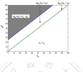
(18) Chapter 2 Testing the null hypothesis of 政治大 equality 立 ‧. ‧ 國. 學. Assume two independent Poisson random samples within a fixed duration,. y. sit. 𝑖𝑖𝑑. Nat. (𝑌11 , ⋅ ⋅ ⋅ , 𝑌1𝑛1 ), (𝑌21 , ⋅ ⋅ ⋅ , 𝑌2𝑛2 ), 𝑖𝑖𝑑. io. al. er. 𝑌1𝑖 ∼ 𝑃 𝑜𝑖(𝜆1 ), 𝑌2𝑗 ∼ 𝑃 𝑜𝑖(𝜆2 ), for 𝑖 = 1 ⋅ ⋅ ⋅ 𝑛1 , 𝑗 = 1 ⋅ ⋅ ⋅ 𝑛2 ,. v. n. where 𝑃 𝑜𝑖(⋅) is a Poisson distribution with the mean rate (⋅). Then, the full. Ch. parameter space is the first quadrant on ℛ2 ,. engchi. i Un. Ω = {(𝜆1 , 𝜆2 )∣𝜆1 > 0, 𝜆2 > 0}. This study mainly focuses on three types of one-sided hypothesis testing problems on comparing the two Poisson distributions. The first two problems are the so-called superiority tests, while the third one is the non-inferiority test. An essential difference between these problems is the extent of the associated null parameter space, which determines the complexity of the problem as explained in Chapter 1. See Figure 2.1 for the plots of the three null parameter spaces. In this chapter, for simplicity, we consider the null hypothesis of equality. The associated null parameter space includes only 7.

(19) the diagonal (Ω01 = {0 < 𝜆1 = 𝜆2 } in Figure 2.1). Next chapter, the test of superiority will be explored. The correspondent null space be extended to Ω02 which is the region above and including the diagonal line. Subsequently, the problem of testing non-inferiority correspondent to the null space Ω03 will be studied.. 2.1. Statistical Hypothesis and Test Statistics. 政治大. If prior knowledge indicates the equality of the two population, the statistical. 立. ∑𝑛1. 𝑖=1. 𝑌1𝑖 , 𝑌2 =. vs.. 𝐻1 : 𝜆1 > 𝜆2 .. ∑𝑛2. 𝑗=1. 𝑌2𝑗 are sufficient statistics, and. ‧. It’s seen that 𝑌1 =. 𝐻01 : 𝜆1 = 𝜆2 ,. 學. ‧ 國. hypothesis can be expressed as follows,. er. io. sit. y. Nat. the maximum likelihood estimator(MLE) of 𝛿 = 𝜆1 − 𝜆2 can be derived as 𝛿ˆ = 𝑌¯1 − 𝑌¯2 , where 𝑌¯1 , 𝑌¯2 are the MLE of 𝜆1 and 𝜆2 under Ω, respectively. ˆ Dividing the MLE 𝛿ˆ by its estimated asymptotic standard error 𝑠𝑒(𝛿),. n. al. Ch. one obtains the Wald’s test statistic,. e n gˆc h i. 𝑍=. 𝛿. ˆ 𝑠𝑒(𝛿). i Un. v. ,. ˆ is obtained by plugging some consistent estimators of 𝜆1 , 𝜆2 in where 𝑠𝑒(𝛿) ˆ In general, two common estimators are employed, the standard error of 𝛿. one with constrained MLE is 𝑌¯1 − 𝑌¯2 𝑍𝑅 = √ , ˜0 ˜0 𝜆 𝜆 + 𝑛2 𝑛1 ˜0 = where 𝜆. 𝑌1 +𝑌2 𝑛1 +𝑛2. is RMLE(restricted maximum likelihood estimator)under. 8.

(20) 𝐻01 : 𝜆1 = 𝜆2 = 𝜆. The other one with unconstrained MLE is 𝑌¯1 − 𝑌¯2 𝑍𝑈 = √ . 𝑌¯2 𝑌¯1 + 𝑛2 𝑛1 On the other hand, when testing the equality of two normal means, the twoindependent sample 𝑇 -test is commonly used. We will study the applicability of this test in the comparison of Poisson means. Let 𝑆12 , 𝑆22 be the sample variances of the two random samples, respectively. The two-independentsample 𝑇 statistic is 𝑇 =. 政治大. (𝑛1 − 1)𝑆12 + (𝑛2 − 1)𝑆22 𝑌¯ − 𝑌¯2 √1 , where 𝑆𝑝2 = 𝑛1 + 𝑛2 − 2 𝑆𝑝 𝑛11 + 𝑛12. 立. ‧ 國. 學. is the pooled sample variance. The null hypothesis 𝐻01 is rejected if a sufficiently large value of 𝑍 or 𝑇 is observed.. ‧. The asymptotic 𝑝-values of the two Wald’s tests can be computed straight-. y. Nat. forward under normality, while the asymptotic 𝑝-value of the 𝑇 -test is found. io. sit. under a 𝑡-distribution with degrees of freedom (𝑛1 + 𝑛2 − 2). The theoretical. n. al. er. performance of the asymptotic power function of the three 𝑝-values will be studied in next section.. 2.2. Ch. engchi. i Un. v. Asymptotic 𝑝-values. In the following, the asymptotic 𝑝-values of the observed 𝑧𝑅 , 𝑧𝑈 , 𝑡0 are 𝑝𝐴,𝑅 = 1 − Φ(𝑧𝑈 ), 𝑝𝐴,𝑈 = 1 − Φ(𝑧𝑅 ), 𝑝𝑇 = 1 − 𝑡(𝑛1 +𝑛2 −2) (𝑡0 ) where Φ(⋅) is the distribution function of 𝑁 (0, 1), and 𝑡𝜈 (⋅) is the 𝑡-distribution with degrees of freedom 𝜈 . The null hypothesis is rejected if the 𝑝-value is not greater than the significance level 𝛼. In the following, we will explore the 9.

(21) 政治大. 立. ‧ 國. 學. Figure 2.1: The joint parameter space Ω is all, the null parameter space Ω01 for testing the equality, and the null parameter space Ω02 for testing superiority, the null parameter space Ω03 for testing non-inferiority.. deriving formula of required sample sizes for these tests.. Nat. sit. y. ‧. validity and asymptotic power function of the three asymptotic tests, and. al. er. io. Theorem 1. Let 𝛿0 be the true value of 𝛿, and 𝜌 = 𝑛1 /𝑛2 ∈ (0, 1) be the. iv n U 𝑑. n. sample size fraction of the first group to the second group. As 𝑛1 , 𝑛2 → ∞, 𝑑. Ch. engchi. 𝑍𝑅 ⋅ 𝜎 − 𝜇 → 𝑁 (0, 1) and 𝑍𝑈 − 𝜇 → 𝑁 (0, 1). In which, 𝜇= √. 𝛿0 (1+𝜌)𝜆2 +𝛿0 𝑛2 𝜌. √ ,. 𝜎=. (1 + 𝜌)𝜆2 + 𝜌𝛿0 . (1 + 𝜌)𝜆2 + 𝛿0. At significance level 𝛼, 𝐻01 is rejected if the test statistic exceeds 𝑧𝛼 , where 𝑧𝛼 is the 100(1 − 𝛼)%-th percentile of 𝑁 (0, 1). Then the asymptotic power functions of 𝑍𝑅 , 𝑍𝑈 can be found as follows, 𝛽¯𝑍𝑅 (𝛿0 , 𝜆2 , 𝑛2 , 𝜌) = 1 − Φ(𝑧𝛼 𝜎 − 𝜇), 10. 𝛽¯𝑍𝑈 (𝛿0 , 𝜆2 , 𝑛2 , 𝜌) = 1 − Φ (𝑧𝛼 − 𝜇) ..

(22) Under 𝐻01 , 𝛿0 = 0, then 𝜇 = 0, 𝜎 = 1, and further 𝛽¯𝑍𝑈 = 𝛽¯𝑍𝑅 = 𝛼. That is, both the two asymptotic tests successfully control their type I error rate at the significance level. The correspondent 𝑝-values are called asymptotic valid. When 𝛿0 > 0, 𝜇 > 0, the asymptotic power 𝛽¯𝑍𝑈 can be shown always greater than 𝛼. It indicates that the testing procedure 𝑍𝑈 is an unbiased test approximately. Nevertheless, the unbiasedness of 𝑍𝑅 is not always true. When the first group has a smaller size than the second group, i.e. 𝜌 ≤ 1, 𝜎 ≤ 1, the asymptotic power 𝛽¯𝑍 is always above the nominal level 𝛼 and. 政治大 increases as 𝛿 . On the contrary, if 𝜌 > 1, the power may not exceed the 立 nominal level. In the following we explore the behavior of the asymptotic 𝑅. 0. ‧ 國. 學. ‧. power 𝛽¯𝑍𝑅 at some extreme 𝜆2 as 𝛿0 > 0, 𝜌 > 1. As 𝜆2 approaches to infinity, √ 𝛿0 𝜆2 (1 + 𝜌) + 𝜌𝛿0 𝜇= √ → 0, 𝜎 = → 1. 𝜆2 (1+𝜌)+𝛿0 𝜆2 (1 + 𝜌) + 𝛿0 𝑛2 𝜌. y. Nat. sit. n. al. er. io. Then the asymptotic power of 𝑍𝑅 converges to the level 𝛼. As 𝜆2 → 0, √ √ 𝛿0 𝜆2 (1 + 𝜌) + 𝜌𝛿0 √ 𝜇= √ → 𝑛2 𝜌𝛿0 , 𝜎 = → 𝜌. 𝜆2 (1+𝜌)+𝛿0 𝜆2 (1 + 𝜌) + 𝛿0 𝑛2 𝜌. Hence,. Ch. engchi. i Un. v. ( √ ) √ lim 𝛽¯𝑍𝑅 = 1 − Φ 𝑧𝛼 𝜌 − 𝑛2 𝜌𝛿0 .. 𝜆2 →0. (2.1). In this case, one can see that 𝛽¯𝑍𝑅 increases as 𝛿0 increases. However it’s easy to derive that the power is less than 𝛼 when { √ } 𝑧𝛼 ( 𝜌 − 1) 2 𝛿0 < . √ 𝑛2 𝜌 Hence, 𝑍𝑅 tends to be biased when the sample sizes are extremely unbalanced and the means of group are relatively small, i.e. 𝜌 >> 1, 𝜆1 ≈ 0, 𝜆2 ≈ 0. See Figure 2.2 for the plots of the asymptotic power function of 𝑍𝑅 for 11.

(23) 𝜌 = 8, 20, 50, 𝜆2 = 0.03 and 𝑛2 = 10. In summary, 𝑍𝑅 is not always an unbiased test for 𝜌 > 1. In the next theorem, the asymptotic distribution of 𝑇 is shown the same as that of 𝑍𝑅 in this Poisson problem. It’s known that the mean and the variance coincide in a Poisson population. Hence the two test statistics use a sample estimate of standard error of 𝛿ˆ in the denominator under a common constraint.. 治政 Theorem 2. Let 𝛿 be the true value of 𝛿, and 大𝜌 = 𝑛 /𝑛 be the sample size fraction of the first立 group to the second group. As 𝑛 , 𝑛 → ∞, 1. 2. 1. 2. 學. ‧ 國. 0. 𝑑. 𝑇 𝜎 − 𝜇 → 𝑁 (0, 1).. ‧ sit. y. Nat. When 𝑛1 , 𝑛2 are sufficiently large, the critical value of the 𝑇 test approximates to that of the Wald test, 𝑡(𝑛1 +𝑛2 −2,𝛼) ≈ 𝑧𝛼 . In addition, from. io. n. al. er. Theorem 2, 𝑇 and 𝑍𝑅 have the same asymptotic distribution. Consequently,. i Un. v. the asymptotic power of 𝑇 can be derived to be equal to the power of 𝑍𝑅 ,. Ch. engchi. 𝛽¯𝑇 (𝛿0 , 𝜆2 , 𝜌, 𝑛2 ) = 𝛽¯𝑍𝑅 = 1 − Φ (𝑧𝛼 𝜎 − 𝜇) . Hence 𝑇 has the same performance as 𝑍𝑅 approximately. According to the discussion in previous paragraphs, 𝑇 is a valid test, and is unbiased as 𝜌 ≤ 1. As 𝜌 > 1, 𝑇 is not necessarily unbiased. Based on the power function of a testing procedure, the necessary sample size for achievement of a prespecified power at some alternative setting at significance level can be further determined. Given 𝜌, to achieve a prespecified power level 1 − 𝛽0 at 𝜆2 , 𝛿0 > 0, the minimal sample size of the second 12.

(24) group required for the 𝑍𝑈 and 𝑍𝑅 at significant level 𝛼 is given as { }2 { } 𝑧𝛼 𝜎 + 𝑧𝛽0 𝜆2 (1 + 𝜌) + 𝛿0 ∗ 𝑛2,𝑍𝑅 ≥ , 𝛿0 𝜌. (2.2). and 𝑛∗2,𝑍𝑈. { ≥. 𝑧𝛼 + 𝑧𝛽0 𝛿0. }2 {. 𝜆2 (1 + 𝜌) + 𝛿0 𝜌. } ,. (2.3). respectively. The size of the first group is found as 𝑛∗1 = [𝑛∗2 ⋅ 𝜌] + 1, in which [𝑎] = 𝑞, the 𝑞 is the maximum integer less than or equal to 𝑎. The formulae of sample sizes for 𝑇 is equivalent to the equation (2.2).. 政治大 It can be seen that the powers and sample size formulae of the three 立 tests mainly differ in the multiple of 𝑧 , 𝜎. When 𝜌 = 1, the sample sizes 𝛼. ‧ 國. 學. are balanced, 𝜎 = 1 and the three tests are equivalent in terms of the power function and the sample size formula. When 𝛿0 = 0, all 𝛽¯𝑍 = 𝛽¯𝑇 = 𝛽¯𝑍 = 𝛼. 𝑅. 𝑈. ‧. When 𝛿0 > 0, we discover that 𝛽¯𝑍𝑈 < 𝛽¯𝑍𝑅 = 𝛽¯𝑇 if 𝜌 < 1, 𝛽¯𝑍𝑈 > 𝛽¯𝑍𝑅 = 𝛽¯𝑇 , if. y. Nat. 𝜌 > 1. See Figure 2.3. It indicates that the 𝑍𝑅 − /𝑇 -tests are more powerful. sit. and required less observations for a specified power than the 𝑍𝑈 -test when. al. er. io. there are less observations in the first group. The result is opposite when the. v. n. samples size of the first group is more than that of the second group. Hence,. Ch. i Un. when the sampling cost for a subject from the first group is more expensive. engchi. than from the second group, one may consider a study of 𝜌 < 1, and the use of 𝑍𝑅 or 𝑇 is suggested. In this study, the sampling fraction 𝜌 ∈ (0, ∞) is considered a fixed constant exactly or approximately. It requires that the two group sizes 𝑛1 , 𝑛2 have the same converging rates. Otherwise, as both sizes converge to infinity, the statistic correspondent to the larger sample converges to a constant faster than others. The subsequent asymptotic distribution of the testing statistic becomes trivial and is less worthy to derive. On the other hand, in the design stage, the sampling fraction 𝜌 should be specified a priori for 13.

(25) sample size determination. In practice, the information, as well as 𝜆2 , 𝛿0 , are obtained after a consultation with experts of the related field and after taking consideration of a realistic situation on applications. When testing a parameter of a discrete distribution, a continuity correction is often added in the test statistic when one applies an approximation by some continuous distribution. The continuity correction revised by Pirie and Hamdan (1972) is employed in the Poisson problem. It’s known that given an unbiased and sufficient estimator 𝛿ˆ for 𝛿, the continuity corrected. 政𝛿ˆ − 𝑏治大 ,. test statistic is. 1 2. 立. ˆ 𝑠𝑒(𝛿). ‧ 國. 學. provided that the support of 𝛿ˆ has equal spacings with space 𝑏.. ‧. Pirie and Hamdan (1972) indicated that for two independent Poisson random samples, the MLE 𝛿ˆ has equal spacings if one of 𝑛1 , 𝑛2 is an integer. Nat. sit. y. multiple of the other. Specifically, when 𝑛1 = 𝑛2 , 𝑏 = 1. In the following. er. io. theorem, we extend the results of Pirie and Hamdan (1972) to any 𝑛1 , 𝑛2 .. al. n. iv n C ˆ Theorem 3. For any 𝑛1 , h 𝑛2e , the sampling n g c h i Udistribution of 𝛿 has equal. spacings with space. 1 , 2𝑚 where 𝑚 is the least common multiple of 𝑛1 , 𝑛2 . 𝑏=. Consequently, the continuity-corrected two Wald’s test and 𝑇 -test are defined as 𝑍𝑐 =. 𝛿ˆ −. 1 2𝑚. ˆ 𝑠𝑒(𝛿). , 𝑇𝑐 = 𝑠𝑝. 𝛿ˆ − √. 1 𝑛1. 1 2𝑚. +. , 1 𝑛2. respectively. In which 𝑍𝑐 can be either 𝑍𝑅,𝑐 or 𝑍𝑈,𝑐 . 14.

(26) 2.3. Exact 𝑝-values. When the sample sizes are insufficient or the mean values are relatively small, exact testing procedures are more adequate than asymptotic ones. Given a realization of a test statistic, an exact 𝑝-value is defined and calculated under the exact null distribution. In many applications, the null distribution often involves an unknown nuisance parameter(s). Here, both the Wald statistics 𝑍𝑈 , 𝑍𝑅 are functions of the sufficient statistics (𝑌1 , 𝑌2 ). Under the. 政治大. null hypothesis, 𝐻01 : 𝜆1 = 𝜆2 = 𝜆 > 0, 𝑌1 , 𝑌2 independently follow a Poisson distribution with mean 𝑛1 𝜆, 𝑛2 𝜆, respectively. Given an observed 𝑧0 of the. 立. Wald statistic 𝑍, where 𝑍 can be either 𝑍𝑈 or 𝑍𝑅 , an exact 𝑝-value is defined. 𝑝𝜆 (𝑧0 ) = 𝑃 (𝑍 ≥ 𝑧0 ∣𝜆1 = 𝜆2 = 𝜆) =. ∑∑. ‧. ‧ 國. value 𝜆,. 學. under the true null distribution, which involves the unknown common mean. 𝑝𝑜𝑖(𝑦1 , 𝑛1 𝜆)𝑝𝑜𝑖(𝑦2 , 𝑛2 𝜆)𝐼{𝑍≥𝑧0 } ,. 𝑦1 ≥0 𝑦2 ≥0. sit. y. Nat. (2.4). er. io. where 𝑝𝑜𝑖(𝑦, 𝜆′ ) is the probability function of Poisson distribution with mean. al. n. iv n C In the following, several testing procedures to U with unknown nuisance he n g c h i deal parameters in literature are reviewed.. 𝜆′ and 𝐼 is the indicator function. The common 𝜆 is a nuisance parameter.. Casella and Berger (1990) defined the following standard 𝑝-value that considers the most conservative scenario and guarantees the validity, 𝑝𝑠 =. sup. 𝑃 (𝑍 ≥ 𝑧0 ∣𝜆1 = 𝜆2 = 𝜆),. 𝜆1 ,𝜆2 ∈Ω01. where Ω01 = {(𝜆1 , 𝜆2 ) : 𝜆1 = 𝜆2 > 0} is the null parameter space of 𝐻01 . Ω01 is unbounded in a Poisson problem, hence the computation of the standard 𝑝-value is difficult in real-world applications. In addition, not taking the data 15.

(27) information into consideration, one may obtain an unnecessarily conservative conclusion. To ease the computational burden brought by searching the supremum over an infinite interval, Berger and Boos (1994) proposed a confidence-set 𝑝value and showed that it is valid. The confidence-set 𝑝-value is the supremum over a confidence-set of the nuisance parameter. Here, given an observation 𝑧𝑅 of 𝑍𝑅 , the confidence-set 𝑝-value is defined as. 政治大. (𝛾) 𝑝𝐶𝐼,𝑅 = sup 𝑃 (𝑍𝑅 ≥ 𝑧𝑅 ∣ 𝜆1 = 𝜆2 = 𝜆) + 𝛾,. 𝜆∈𝐶𝛾. 立. (2.5). where 𝐶𝛾 is a 100(1 − 𝛾)% confidence interval for the nuisance parameter 𝜆.. ‧ 國. 學. On the other hand, given 𝑧𝑈 , the confidence-set 𝑝-value based on 𝑍𝑈 is (𝛾) = sup 𝑃 (𝑍𝑈 ≥ 𝑧𝑈 ∣ 𝜆1 = 𝜆2 = 𝜆) + 𝛾. 𝑝𝐶𝐼,𝑈. (2.6). ‧. 𝜆∈𝐶𝛾. In which, 𝛾 is a positive real number and is far less than 𝛼 for a non-trivial. Nat. sit. y. conclusion. In this study, we consider the following 100(1 − 𝛾)% exact con-. al. er. io. fidence interval 𝐶𝛾 of 𝜆,. v. n. 1 (𝜒2 , 𝜒2 ), 2(𝑛1 + 𝑛2 ) (1−𝛾/2, 2(𝑌1 +𝑌2 )) (𝛾/2, 2(𝑌1 +𝑌2 +1)). Ch. engchi. i Un. where 𝜒2𝛼,𝑣 is the 100(1 − 𝛼)-th percentile of a chi-square distribution with degrees of freedom 𝑣 (Casella and Berger, 1990). The confidence interval is based on the following equivalent relationship between Poisson and Chisquare random variables, 𝛾 = 𝑃 (𝑌 ≤ 𝑦0 ) = 𝑃 (𝜒22(𝑦0 +1) > 2(𝑛1 + 𝑛2 )𝜆), 2 𝛾 = 𝑃 (𝑌 ≥ 𝑦0 ) = 𝑃 (𝜒22𝑦0 < 2(𝑛1 + 𝑛2 )𝜆), 2 where 𝑌 follows 𝑃 𝑜𝑖((𝑛1 + 𝑛2 )𝜆), 𝜒22(⋅) is a random variable with degrees of freedom 2(⋅).. 16.

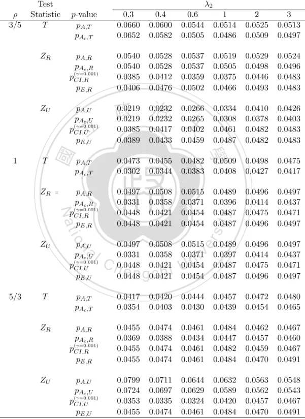
(28) Krishnamoorthy and Thomson (2004) proposed an alternative exact 𝑝˜ 0 of the nuisance parameter 𝜆. That is, given value by using the RMLE 𝜆 𝑧𝑅 , 𝑧𝑈 , the estimated 𝑝-value are defined as ˜ 0 ), 𝑝𝐸,𝑈 = 𝑃 (𝑍𝑈 ≥ 𝑧𝑈 ∣ 𝜆 ˜ 0 ), 𝑝𝐸,𝑅 = 𝑃 (𝑍𝑅 ≥ 𝑧𝑅 ∣ 𝜆 respectively. The estimated 𝑝-value has great reduction in computation and performs well empirically. Although the estimator owns many pleasant properties in the inference of point estimation under 𝐻01 , but the resultant 𝑝-value does not guarantee a valid test theoretically.. 政治大. As the Wald statistic depends on the data only through the two sufficient. 立. ∑∑. 學. 𝑝, is given by. ‧ 國. statistics (𝑌1 , 𝑌2 ), the exact power of the test correspondent to the 𝑝-value,. 𝑝𝑜𝑖(𝑦1 , 𝑛1 𝜆1 )𝑝𝑜𝑖(𝑦2 , 𝑛2 𝜆2 )𝐼{𝑝≤𝛼} .. ‧. 𝑦1 ≥0 𝑦2 ≥0. Given a predetermined power level 1 − 𝛽0 at some specific 𝜆2 and 𝛿0 > 0 , the. sit. y. Nat. required sample size of the second group is the smallest integers such that. n. al. er. io. the exact power achieves the level, and it is found as follows ∑∑ 𝑛∗2 = min{𝑛2 : 𝑝𝑜𝑖(𝑦1 , ([𝑛2 𝜌] + 1)(𝜆2 + 𝛿0 ))𝑝𝑜𝑖(𝑦2 , 𝑛2 𝜆2 )𝐼{𝑝≤𝛼} ≥ 1 − 𝛽0 }, 𝑦1 ≥0 𝑦2 ≥0. Ch. engchi. i Un. v. (2.7). for some 𝜌 > 0. Further 𝑛∗1 = [𝑛∗2 𝜌] + 1.. 2.4. Numerical study. In this section, we investigate the performance of the two test statistics 𝑍𝑅 , 𝑍𝑈 , as well as 𝑇 . The asymptotic testing procedures by using the asymptotic 𝑝−values are considered. The effect of a continuity correction are explored in these asymptotic tests. Denote the 𝑝-value as 𝑝𝐴 if it is without a 17.

(29) continuity correction; as 𝑝𝐴𝑐 if it is with a continuity correction term. The exact tests by using the confidence-set 𝑝-value, denoted as 𝑝𝐶𝐼 , and the estimated 𝑝-value, denoted as 𝑝𝐸 , of 𝑍𝑅 , 𝑍𝑈 are further studied. As described in previous section, the calculation of the exact power is straightforward when the test statistic depends on the data only through the two sufficient statistics 𝑌1 , 𝑌2 . Here, except the 𝑇 -test, the exact type I error rate and the exact power of each test are calculated. The power of the 𝑇 -test is found through 100, 000 replicates. In this numerical analysis, we consider 𝜆2 = 0.3, 0.4, 0.6, 1, 2, 3, 𝑛2 = 10, 30, 𝛿0 = 0, 1, 𝜌 = 3/5, 1, 5/3 and 𝛼 = 0.05.. 政治大 The required samples sizes of the second group to achieve 1 − 𝛽 立 power at 𝛿 = 0.6, 1 are provided in Table 2.5-2.10.. The calculated type I error rate and power are presented in Table 2.1-2.4. 0. = 80%. 0. ‧ 國. 學. We first compare the three asymptotic tests in Table 2.1 to 2.4. Although. ‧. 𝑍𝑅 and 𝑇 are found to have different results in the finite sample cases from. y. Nat. the tables, we find that the two tests have quite consistent patterns. It jus-. sit. tifies the theoretical results given in Section 2.2 that the two test statistics. al. er. io. have the same asymptotic distributions. Theoretically, at 𝛿0 = 0 the asymp-. v. n. totic sizes of the three tests are independent of 𝜌 and equal to the nominal. Ch. i Un. significance level 𝛼. However, the finite-sample results in Table 2.1 and Table. engchi. 2.3 appear to be more consistent with the asymptotic power functions under the alternative hypothesis. When 𝜌 = 3/5 < 1, 𝑍𝑅 and 𝑇 have more chance to reject the null hypothesis than 𝑍𝑈 . The trend becomes the opposite when 𝜌 > 1. Basically, the type I error rate of the three tests sometimes exceed the nominal level 𝛼 = 5%. Although as the sample sizes increase, there are some improvement in the type I error rate, the differences are not obvious. When 𝜌 = 3/5, the sizes of 𝑍𝑅 and 𝑇 are not well-controlled at 𝛼 = 5%, and 𝑇 is more liberal than 𝑍𝑅 at small 𝜆2 and 𝑛2 = 10. For 𝜌 = 5/3, the inflation of the type I error rate of 𝑍𝑈 is even worse. For the three tests, at 𝜌 > 1, 𝜌 < 1, adding a continuity correction or increasing the sample size 18.

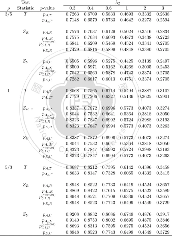
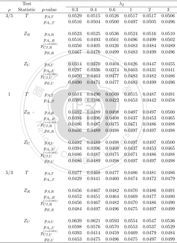
(30) entail limited improvement. Overall speaking, 𝑍𝑅 and 𝑇 is more robust to the choice of 𝜌 than 𝑍𝑈 . 𝑍𝑈 is too liberal for 𝜌 > 1 and is too conservative for 𝜌 < 1. Next the two exact 𝑝-values, 𝑝𝐶𝐼 , 𝑝𝐸 , are studied. Note that in finding the confidence-set 𝑝-value, the supremum is searched over 16 grids of the confidence interval of the common mean value 𝜆. Moreover, we consider 𝛾 = 0.001. Table 2.1 and 2.3 show that the two exact approaches have their type I error rate well-controlled. The confidence-interval 𝑝-value is more. 政治大 greatly reduced for the estimated 𝑝-value. One should keep in mind that the 立 estimated 𝑝-value is not a valid test theoretically. Although in these selected. conservative than the estimated 𝑝-value. The computations involved are. ‧ 國. 學. scenarios of our simulation, its type I error rate does not exceed the nominal level. It is possible that the estimated 𝑝-value has an inflated type I error. ‧. rate in other cases.. y. Nat. sit. Table 2.5-2.10 present the required sample size of the second group for. al. er. io. 80% power at 𝛿0 = 0.6, 1.0. The results for the three asymptotic tests are. v. n. based on the asymptotic sample size formulae (2.2) and (2.3). For the two. Ch. i Un. exact tests, the figures are the minimal integers such that the exact power. engchi. achieves the level by (2.7). All the tests need less required sample size of the second group for 80% power when the 𝛿0 increases. Between the three asymptotic tests, 𝑍𝑈 needs a slightly smaller sample than 𝑍𝑅 and 𝑇 for 𝜌 > 1. On the contrary, however, with the smaller sample size, the exact type I error rate of three asymptotic tests often exceeds the nominal level 𝛼. The inflation is more severe in the application of 𝑍𝑈 and showed limited improvement with the continuity correction. Moreover, the sample sizes obtained for the two exact tests are near that of the asymptotic tests and the differences are within 3 units in all cases. With 19.

(31) the calculated sample size, every exact test achieves the prespecified power level and has a well-controlled type I error rate. In summary, although the exact tests are more time-consuming, they guarantee more adequate statistical conclusions. The asymptotic sample sizes (2.2) and (2.3) can be regarded as an efficient alternative of (2.7) for the exact tests. A much quicker solution can be obtained and the result is found to be close to the exact sample size.. 立. 政治大. ‧. ‧ 國. 學. n. er. io. sit. y. Nat. al. Ch. engchi. 20. i Un. v.

(32) Table 2.1: The type I error rate (𝛿0 = 0) of asymptotic 𝑝-value test (𝑝𝐴 ) and exact 𝑝-value test (𝑝𝐶𝐼 , 𝑝𝐸 ) based on 𝑇, 𝑍𝑅 , 𝑍𝑈 respectively for 𝑛2 = 10. 𝜆2 0.3 0.0660 0.0652. 0.4 0.0600 0.0582. 0.6 0.0544 0.0505. 1 0.0514 0.0486. 2 0.0525 0.0509. 3 0.0513 0.0497. 𝑝𝐴,𝑅 𝑝𝐴𝑐 ,𝑅. 0.0540 0.0540 0.0385 0.0406. 0.0528 0.0528 0.0412 0.0476. 0.0537 0.0537 0.0359 0.0502. 0.0519 0.0505 0.0375 0.0466. 0.0529 0.0498 0.0446 0.0493. 0.0524 0.0496 0.0483 0.0483. 0.0334 0.0308 0.0461 0.0487. 0.0410 0.0378 0.0482 0.0482. 0.0426 0.0403 0.0483 0.0483. 0.0498 0.0427. 0.0475 0.0417. 0.0496 0.0414 0.0475 0.0496. 0.0497 0.0437 0.0471 0.0497. (𝛾=0.001) 𝑝𝐶𝐼,𝑅 𝑝𝐸,𝑅. 𝑍𝑈. 𝑝𝐴,𝑈 𝑝𝐴𝑐 ,𝑈. 立. 𝑇. 0.0459. 𝑝𝐴,𝑇 𝑝𝐴𝑐 ,𝑇. 0.0473 0.0302. 0.0455 0.0344. 0.0482 0.0383. 0.0509 0.0408. 𝑝𝐴,𝑅 𝑝𝐴𝑐 ,𝑅. 0.0497 0.0331 0.0448 0.0448. 0.0508 0.0358 0.0421 0.0421. 0.0515 0.0371 0.0454 0.0454. 0.0489 0.0396 0.0487 0.0487. 0.0497 0.0331 0.0448 0.0448. 0.0508 0.0358 0.0421 0.0421. 0.0515 0.0371 0.0454 0.0454. 0.0489 0.0397 0.0487 0.0487. 0.0496 0.0414 0.0475 0.0496. 0.0497 0.0437 0.0471 0.0497. Nat. 0.0433. (𝛾=0.001) 𝑝𝐶𝐼,𝑅 𝑝𝐸,𝑅. io. 𝑝𝐴,𝑈 𝑝𝐴𝑐 ,𝑈. al. n. 𝑍𝑈. (𝛾=0.001) 𝑝𝐶𝐼,𝑈 𝑝𝐸,𝑈. 5/3. Ch. ‧. 𝑍𝑅. 0.0389. 學. 1. ‧ 國. (𝛾=0.001) 𝑝𝐶𝐼,𝑈 𝑝𝐸,𝑈. 0.0219 0.0232 治 0.0266 政 0.0219 0.0232 0.0265 大 0.0385 0.0417 0.0402. y. 𝑍𝑅. 𝑝-value 𝑝𝐴,𝑇 𝑝𝐴𝑐 ,𝑇. sit. Test Statistic 𝑇. er. 𝜌 3/5. n engchi U. iv. 𝑇. 𝑝𝐴,𝑇 𝑝𝐴𝑐 ,𝑇. 0.0417 0.0354. 0.0420 0.0403. 0.0444 0.0430. 0.0457 0.0439. 0.0472 0.0454. 0.0480 0.0465. 𝑍𝑅. 𝑝𝐴,𝑅 𝑝𝐴𝑐 ,𝑅. 0.0455 0.0369 0.0455 0.0455. 0.0474 0.0388 0.0474 0.0474. 0.0461 0.0434 0.0461 0.0461. 0.0484 0.0447 0.0482 0.0484. 0.0462 0.0457 0.0459 0.0470. 0.0467 0.0460 0.0467 0.0491. 0.0799 0.0724 0.0353 0.0455. 0.0711 0.0697 0.0335 0.0474. 0.0644 0.0629 0.0324 0.0461. 0.0632 0.0589 0.0420 0.0484. 0.0563 0.0562 0.0457 0.0470. 0.0548 0.0543 0.0467 0.0491. (𝛾=0.001) 𝑝𝐶𝐼,𝑅 𝑝𝐸,𝑅. 𝑍𝑈. 𝑝𝐴,𝑈 𝑝𝐴𝑐 ,𝑈 (𝛾=0.001) 𝑝𝐶𝐼,𝑈 𝑝𝐸,𝑈. 21.



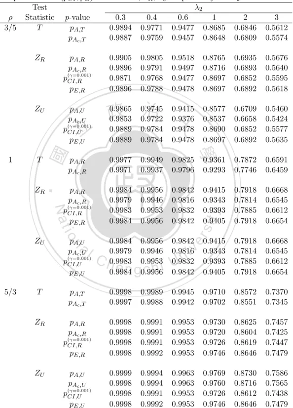
(35) Table 2.4: The type I error rate (𝛿0 = 1) of asymptotic 𝑝-value test (𝑝𝐴 ) and exact 𝑝-value test (𝑝𝐶𝐼 , 𝑝𝐸 ) based on 𝑇, 𝑍𝑅 , 𝑍𝑈 respectively for 𝑛2 = 30. 𝜆2 0.3 0.9894 0.9887. 0.4 0.9771 0.9759. 0.6 0.9477 0.9457. 1 0.8685 0.8648. 2 0.6846 0.6809. 3 0.5612 0.5574. 𝑝𝐴,𝑅 𝑝𝐴𝑐 ,𝑅. 0.9905 0.9896 0.9871 0.9896. 0.9805 0.9791 0.9768 0.9788. 0.9518 0.9497 0.9477 0.9478. 0.8765 0.8716 0.8697 0.8697. 0.6935 0.6893 0.6852 0.6892. 0.5676 0.5640 0.5595 0.5618. 0.8577 0.8537 0.8690 0.8697. 0.6709 0.6658 0.6852 0.6892. 0.5460 0.5424 0.5577 0.5635. 0.7872 0.7746. 0.6591 0.6459. 0.7918 0.7814 0.7885 0.7918. 0.6668 0.6545 0.6612 0.6654. (𝛾=0.001) 𝑝𝐶𝐼,𝑅 𝑝𝐸,𝑅. 𝑍𝑈. 𝑝𝐴,𝑈 𝑝𝐴𝑐 ,𝑈. 立. 𝑇. 0.9478. 𝑝𝐴,𝑅 𝑝𝐴𝑐 ,𝑅. 0.9977 0.9971. 0.9949 0.9937. 0.9825 0.9796. 0.9361 0.9293. 𝑝𝐴,𝑅 𝑝𝐴𝑐 ,𝑅. 0.9984 0.9979 0.9983 0.9984. 0.9956 0.9946 0.9953 0.9956. 0.9842 0.9816 0.9832 0.9842. 0.9415 0.9343 0.9393 0.9405. 0.9984 0.9979 0.9983 0.9984. 0.9956 0.9946 0.9953 0.9956. 0.9842 0.9816 0.9832 0.9842. 0.9415 0.9343 0.9393 0.9405. 0.7918 0.7814 0.7885 0.7918. 0.6668 0.6545 0.6612 0.6654. Nat. 0.9784. (𝛾=0.001) 𝑝𝐶𝐼,𝑅 𝑝𝐸,𝑅. io. 𝑝𝐴,𝑈 𝑝𝐴𝑐 ,𝑈. al. n. 𝑍𝑈. (𝛾=0.001) 𝑝𝐶𝐼,𝑈 𝑝𝐸,𝑈. 5/3. Ch. ‧. 𝑍𝑅. 0.9889. 學. 1. ‧ 國. (𝛾=0.001) 𝑝𝐶𝐼,𝑈 𝑝𝐸,𝑈. 0.9865 0.9745 治 0.9415 政 0.9853 0.9722 0.9376 大 0.9889 0.9784 0.9478. y. 𝑍𝑅. 𝑝-value 𝑝𝐴,𝑇 𝑝𝐴𝑐 ,𝑇. sit. Test Statistic 𝑇. er. 𝜌 3/5. n engchi U. iv. 𝑇. 𝑝𝐴,𝑇 𝑝𝐴𝑐 ,𝑇. 0.9998 0.9997. 0.9989 0.9988. 0.9945 0.9942. 0.9710 0.9702. 0.8572 0.8551. 0.7370 0.7345. 𝑍𝑅. 𝑝𝐴,𝑅 𝑝𝐴𝑐 ,𝑅. 0.9998 0.9998 0.9998 0.9998. 0.9991 0.9991 0.9991 0.9992. 0.9953 0.9953 0.9953 0.9953. 0.9730 0.9720 0.9726 0.9746. 0.8625 0.8604 0.8619 0.8646. 0.7457 0.7425 0.7447 0.7479. 0.9999 0.9998 0.9998 0.9998. 0.9994 0.9994 0.9991 0.9992. 0.9963 0.9963 0.9953 0.9953. 0.9769 0.9760 0.9726 0.9746. 0.8730 0.8716 0.8612 0.8646. 0.7586 0.7565 0.7438 0.7479. (𝛾=0.001) 𝑝𝐶𝐼,𝑅 𝑝𝐸,𝑅. 𝑍𝑈. 𝑝𝐴,𝑈 𝑝𝐴𝑐 ,𝑈 (𝛾=0.001) 𝑝𝐶𝐼,𝑈 𝑝𝐸,𝑈. 24.

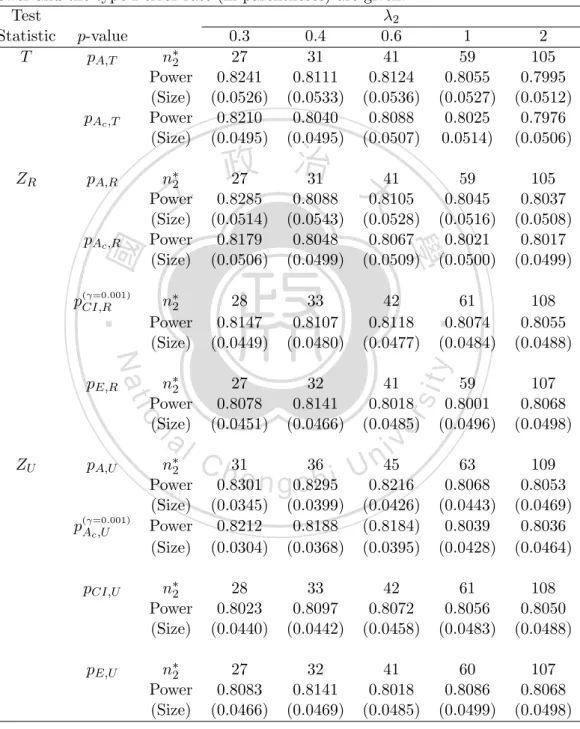
(36) Table 2.5: To achieve 80% power at 𝛿0 = 0.6, the required sample size of the second group 𝑛∗2 of 𝑍𝑅 , 𝑍𝑈 , 𝑇 for 𝜌 = 3/5. Based on the required samples 𝑛∗2 , the power and the type I error rate (in parentheses) are given. Test 𝜆2 Statistic 𝑝-value 0.3 0.4 0.6 1 2 𝑇 𝑝𝐴,𝑇 𝑛∗2 27 31 41 59 105 Power 0.8241 0.8111 0.8124 0.8055 0.7995 (Size) (0.0526) (0.0533) (0.0536) (0.0527) (0.0512) 𝑝𝐴𝑐 ,𝑇 Power 0.8210 0.8040 0.8088 0.8025 0.7976 (Size) (0.0495) (0.0495) (0.0507) 0.0514) (0.0506). (0.0514) 0.8179 (0.0506). (0.0543) 0.8048 (0.0499). 𝑛∗2 Power (Size). 28 0.8147 (0.0449) 27 0.8078 (0.0451). ‧ 國. io. 𝑛∗2 Power (Size). n. al. 𝑍𝑈. 𝑝𝐴,𝑈. (𝛾=0.001) 𝑝𝐴 𝑐 ,𝑈. 𝑛∗2 Power (Size) Power (Size). 33 0.8107 (0.0480). 42 0.8118 (0.0477). 61 0.8074 (0.0484). 108 0.8055 (0.0488). 32 0.8141 (0.0466). 41 0.8018 (0.0485). 59 0.8001 (0.0496). 107 0.8068 (0.0498) 109 0.8053 (0.0469) 0.8036 (0.0464). ‧. Nat. 𝑝𝐸,𝑅. 105 0.8037 (0.0508) 0.8017 (0.0499). 學. (𝛾=0.001) 𝑝𝐶𝐼,𝑅. (0.0528) 0.8067 (0.0509). 59 0.8045 (0.0516) 0.8021 (0.0500). y. 立. 𝑝𝐴𝑐 ,𝑅. 治政 27 31 41 大 0.8285 0.8088 0.8105. 𝑛∗2 Power (Size) Power (Size). sit. 𝑝𝐴,𝑅. er. 𝑍𝑅. iv n C h31 36 45 e n g0.8295 0.8301 c h i U0.8216 (0.0345) 0.8212 (0.0304). (0.0399) 0.8188 (0.0368). (0.0426) (0.8184) (0.0395). 63 0.8068 (0.0443) 0.8039 (0.0428). 𝑝𝐶𝐼,𝑈. 𝑛∗2 Power (Size). 28 0.8023 (0.0440). 33 0.8097 (0.0442). 42 0.8072 (0.0458). 61 0.8056 (0.0483). 108 0.8050 (0.0488). 𝑝𝐸,𝑈. 𝑛∗2 Power (Size). 27 0.8083 (0.0466). 32 0.8141 (0.0469). 41 0.8018 (0.0485). 60 0.8086 (0.0499). 107 0.8068 (0.0498). 25.

(37) Table 2.6: To achieve 80% power at 𝛿0 = 0.6, the required sample size of the second group 𝑛∗2 of 𝑍𝑅 , 𝑍𝑈 , 𝑇 for 𝜌 = 1. Based on the required samples 𝑛∗2 , the power and the type I error rate (in parentheses) are given. Test 𝜆2 Statistic 𝑝-value 0.3 0.4 0.6 1 2 𝑇 𝑝𝐴,𝑇 𝑛∗2 21 25 31 45 79 Power 0.8159 0.8190 0.8014 0.8003 0.7978 (Size) (0.0491) (0.0494) (0.0496) (0.0498) (0.0490) 𝑝𝐴𝑐 ,𝑇 Power 0.7865 0.7933 0.7821 0.7871 0.7904 (Size) (0.0368) (0.0393) (0.0417) (0.0448) (0.0463). (0.0512) 0.7971 (0.0373). (0.0489) 0.8012 (0.0396). 𝑛∗2 Power (Size). 20 0.8070 (0.0454) 20 0.8073 (0.0454). ‧ 國. io. 𝑛∗2 Power (Size). n. al. 𝑍𝑈. 𝑝𝐴,𝑈. 𝑝𝐴𝑐 ,𝑈. 𝑛∗2 Power (Size) Power (Size). 24 0.8088 (0.0487). 31 0.8014 (0.0475). 45 0.8032 (0.0488). 80 0.8025 (0.0489). 24 0.8140 (0.0487). 31 0.8084 (0.0498). ‧. Nat. 𝑝𝐸,𝑅. 79 0.8017 (0.0499) 0.7940 (0.0471). 學. (𝛾=0.001) 𝑝𝐶𝐼,𝑅. (0.0498) 0.7909 (0.0410). 45 0.8059 (0.0505) 0.7931 (0.0448). y. 立. 𝑝𝐴𝑐 ,𝑅. 治 21 25 31 政 0.8244 0.8279 大 0.8084. 𝑛∗2 Power (Size) Power (Size). 45 0.8058 (0.0497). 79 0.8011 (0.0499). sit. 𝑝𝐴,𝑅. er. 𝑍𝑅. iv n C h21 e n g c25h i U 31 0.8244 (0.0512) 0.7971 (0.0373). 0.8279 (0.0489) 0.8012 (0.0396). 0.8084 (0.0498) 0.7909 (0.0410). 45 0.8059 (0.0505) 0.7931 (0.0448). 79 0.8017 (0.0499) 0.7940 (0.0471). (𝛾=0.001) 𝑝𝐶𝐼,𝑈. 𝑛∗2 Power (Size). 20 0.8070 (0.0454). 24 0.8088 (0.0487). 31 0.8014 (0.0475). 45 0.8032 (0.0488). 80 0.8025 (0.0489). 𝑝𝐸,𝑈. 𝑛∗2 Power (Size). 20 0.8073 (0.0454). 24 0.8140 (0.0487). 31 0.8084 (0.0498). 45 0.8058 (0.0497). 79 0.8011 (0.0499). 26.

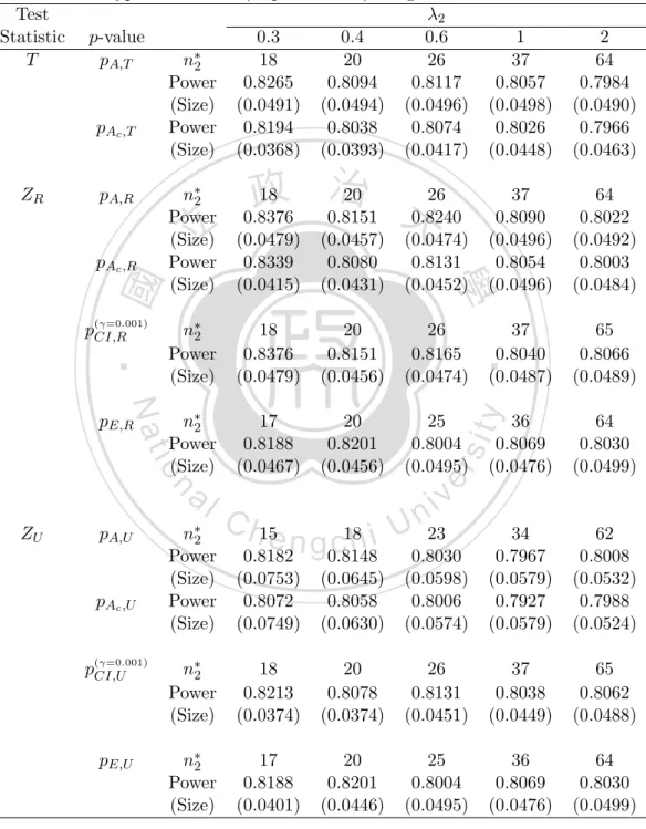
(38) Table 2.7: To achieve 80% power at 𝛿0 = 0.6, the required sample size of the second group 𝑛∗2 of 𝑍𝑅 , 𝑍𝑈 , 𝑇 for 𝜌 = 5/3. Based on the required samples 𝑛∗2 , the power and the type I error rate (in parentheses) are given. Test 𝜆2 Statistic 𝑝-value 0.3 0.4 0.6 1 2 𝑇 𝑝𝐴,𝑇 𝑛∗2 18 20 26 37 64 Power 0.8265 0.8094 0.8117 0.8057 0.7984 (Size) (0.0491) (0.0494) (0.0496) (0.0498) (0.0490) 𝑝𝐴𝑐 ,𝑇 Power 0.8194 0.8038 0.8074 0.8026 0.7966 (Size) (0.0368) (0.0393) (0.0417) (0.0448) (0.0463). (0.0479) 0.8339 (0.0415). (0.0457) 0.8080 (0.0431). 𝑛∗2 Power (Size). 18 0.8376 (0.0479) 17 0.8188 (0.0467). ‧ 國. io. 𝑛∗2 Power (Size). n. al. 𝑍𝑈. 𝑝𝐴,𝑈. 𝑝𝐴𝑐 ,𝑈. 𝑛∗2 Power (Size) Power (Size). 20 0.8151 (0.0456). 26 0.8165 (0.0474). 37 0.8040 (0.0487). 65 0.8066 (0.0489). 20 0.8201 (0.0456). 25 0.8004 (0.0495). ‧. Nat. 𝑝𝐸,𝑅. 64 0.8022 (0.0492) 0.8003 (0.0484). 學. (𝛾=0.001) 𝑝𝐶𝐼,𝑅. (0.0474) 0.8131 (0.0452). 37 0.8090 (0.0496) 0.8054 (0.0496). y. 立. 𝑝𝐴𝑐 ,𝑅. 治 18 20 26 政 0.8376 0.8151 大 0.8240. 𝑛∗2 Power (Size) Power (Size). 36 0.8069 (0.0476). 64 0.8030 (0.0499). sit. 𝑝𝐴,𝑅. er. 𝑍𝑅. iv n C h15 e n g c18h i U 23 0.8182 (0.0753) 0.8072 (0.0749). 0.8148 (0.0645) 0.8058 (0.0630). 0.8030 (0.0598) 0.8006 (0.0574). 34 0.7967 (0.0579) 0.7927 (0.0579). 62 0.8008 (0.0532) 0.7988 (0.0524). (𝛾=0.001) 𝑝𝐶𝐼,𝑈. 𝑛∗2 Power (Size). 18 0.8213 (0.0374). 20 0.8078 (0.0374). 26 0.8131 (0.0451). 37 0.8038 (0.0449). 65 0.8062 (0.0488). 𝑝𝐸,𝑈. 𝑛∗2 Power (Size). 17 0.8188 (0.0401). 20 0.8201 (0.0446). 25 0.8004 (0.0495). 36 0.8069 (0.0476). 64 0.8030 (0.0499). 27.

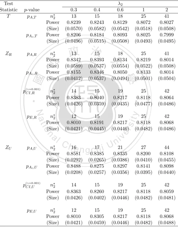
(39) Table 2.8: To achieve 80% power at 𝛿0 = 1, the required sample size of the second group 𝑛∗2 of 𝑍𝑅 , 𝑍𝑈 , 𝑇 for 𝜌 = 3/5. Based on the required samples 𝑛∗2 , the power and the type I error rate (in parentheses) are given. Test 𝜆2 Statistic 𝑝-value 0.3 0.4 0.6 1 2 𝑇 𝑝𝐴,𝑇 𝑛∗2 13 15 18 25 41 Power 0.8239 0.8243 0.8129 0.8072 0.8027 (Size) (0.0570) (0.0582) (0.0542) (0.0518) (0.0508) 𝑝𝐴𝑐 ,𝑇 Power 0.8206 0.8184 0.8093 0.8025 0.7999 (Size) (0.0496) (0.0515) (0.0508) (0.0493) (0.0495). (0.0589) 0.8155 (0.0412). (0.0537) 0.8346 (0.0537). 𝑛∗2 Power (Size). 14 0.8383 (0.0426) 12 0.8010 (0.0421). ‧ 國. io. 𝑛∗2 Power (Size). n. al. 𝑍𝑈. 𝑝𝐴,𝑈. 𝑝𝐴𝑐 ,𝑈. 𝑛∗2 Power (Size) Power (Size). 15 0.8040 (0.0359). 19 0.8217 (0.0435). 25 0.8118 (0.0477). 42 0.8064 (0.0486). 15 0.8191 (0.0445). 19 0.8217 (0.0446). ‧. Nat. 𝑝𝐸,𝑅. 41 0.8014 (0.0508) 0.8014 (0.0504). 學. (𝛾=0.001) 𝑝𝐶𝐼,𝑅. (0.0554) 0.8050 (0.0494). 25 0.8219 (0.0522) 0.8133 (0.0501). y. 立. 𝑝𝐴𝑐 ,𝑅. 治 13 15 18 政 0.8342 0.8393 大 0.8134. 𝑛∗2 Power (Size) Power (Size). 25 0.8118 (0.0482). 42 0.8068 (0.0486). sit. 𝑝𝐴,𝑅. er. 𝑍𝑅. iv n C h16 e n g c17h i U 21 0.8581 (0.0292) 0.8488 (0.0208). 0.8385 (0.0265) 0.8275 (0.0257). 0.8335 (0.0386) 0.8297 (0.0356). 27 0.8200 (0.0410) 0.8141 (0.0395). 44 0.8108 (0.0455) 0.8098 (0.0440). (𝛾=0.001) 𝑝𝐶𝐼,𝑈. 𝑛∗2 Power (Size). 14 0.8363 (0.0426). 15 0.8260 (0.0402). 19 0.8217 (0.0446). 25 0.8118 (0.0482). 42 0.8059 (0.0481). 𝑝𝐸,𝑈. 𝑛∗2 Power (Size). 12 0.8010 (0.0421). 15 0.8305 (0.0459). 19 0.8217 (0.0446). 25 0.8118 (0.0482). 42 0.8068 (0.0488). 28.

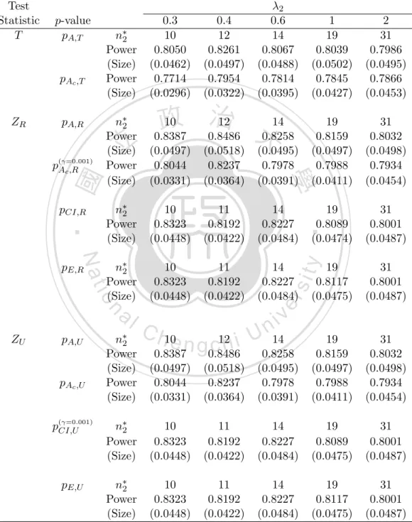
(40) Table 2.9: To achieve 80% power at 𝛿0 = 1, the required sample size of the second group 𝑛∗2 of 𝑍𝑅 , 𝑍𝑈 , 𝑇 for 𝜌 = 1. Based on the required samples 𝑛∗2 , the power and the type I error rate (in parentheses) are given. Test 𝜆2 Statistic 𝑝-value 0.3 0.4 0.6 1 2 𝑇 𝑝𝐴,𝑇 𝑛∗2 10 12 14 19 31 Power 0.8050 0.8261 0.8067 0.8039 0.7986 (Size) (0.0462) (0.0497) (0.0488) (0.0502) (0.0495) 𝑝𝐴𝑐 ,𝑇 Power 0.7714 0.7954 0.7814 0.7845 0.7866 (Size) (0.0296) (0.0322) (0.0395) (0.0427) (0.0453). (0.0518) 0.8237 (0.0364). 𝑛∗2 Power (Size). 10 0.8323 (0.0448) 10 0.8323 (0.0448). io. 𝑛∗2 Power (Size). n. al. 𝑍𝑈. 𝑝𝐴,𝑈. 𝑝𝐴𝑐 ,𝑈. 𝑛∗2 Power (Size) Power (Size). 11 0.8192 (0.0422). 14 0.8227 (0.0484). 19 0.8089 (0.0474). 31 0.8001 (0.0487). 11 0.8192 (0.0422). 14 0.8227 (0.0484). y. Nat. 𝑝𝐸,𝑅. (0.0495) 0.7978 (0.0391). 31 0.8032 (0.0498) 0.7934 (0.0454). ‧. ‧ 國. 𝑝𝐶𝐼,𝑅. (0.0497) 0.8044 (0.0331). 立. 19 0.8159 (0.0497) 0.7988 (0.0411). 學. (𝛾=0.001) 𝑝𝐴 𝑐 ,𝑅. 治 10 12 14 政 0.8387 0.8486 大 0.8258. 𝑛∗2 Power (Size) Power (Size). 19 0.8117 (0.0475). 31 0.8001 (0.0487). sit. 𝑝𝐴,𝑅. er. 𝑍𝑅. iv n C h10 e n g c12h i U 14 0.8387 (0.0497) 0.8044 (0.0331). 0.8486 (0.0518) 0.8237 (0.0364). 0.8258 (0.0495) 0.7978 (0.0391). 19 0.8159 (0.0497) 0.7988 (0.0411). 31 0.8032 (0.0498) 0.7934 (0.0454). (𝛾=0.001) 𝑝𝐶𝐼,𝑈. 𝑛∗2 Power (Size). 10 0.8323 (0.0448). 11 0.8192 (0.0422). 14 0.8227 (0.0484). 19 0.8089 (0.0475). 31 0.8001 (0.0487). 𝑝𝐸,𝑈. 𝑛∗2 Power (Size). 10 0.8323 (0.0448). 11 0.8192 (0.0422). 14 0.8227 (0.0484). 19 0.8117 (0.0475). 31 0.8001 (0.0487). 29.

(41) Table 2.10: To achieve 80% power at 𝛿0 = 1, the required sample size of the second group 𝑛∗2 of 𝑍𝑅 , 𝑍𝑈 , 𝑇 for 𝜌 = 5/3. Based on the required samples 𝑛∗2 , the power and the type I error rate (in parentheses) are given. Test 𝜆2 Statistic 𝑝-value 0.3 0.4 0.6 1 2 𝑇 𝑝𝐴,𝑇 𝑛∗2 9 10 12 16 26 Power 0.8362 0.8329 0.8208 0.8151 0.8105 (Size) (0.0462) (0.0497) (0.0488) (0.0502) (0.0495) 𝑝𝐴𝑐 ,𝑇 Power 0.8275 0.8229 0.8134 0.8111 0.8080 (Size) (0.0296) (0.0322) (0.0395) (0.0427) (0.0453). (0.0404) 0.8605 (0.0394). (0.0474) 0.8422 (0.0388). 𝑛∗2 Power (Size). 8 0.8101 (0.0366) 8 0.8222 (0.0366). ‧ 國. io. 𝑛∗2 Power (Size). n. al. 𝑍𝑈. 𝑝𝐴,𝑈. 𝑝𝐴𝑐 ,𝑈. 𝑛∗2 Power (Size) Power (Size). 9 0.8134 (0.0429). 11 0.8027 (0.0445). 15 0.8023 (0.0474). 26 0.8145 (0.0475). 9 0.8206 (0.0429). 11 0.8099 (0.0481). ‧. Nat. 𝑝𝐸,𝑅. 26 0.8146 (0.0486) 0.8117 (0.0475). 學. (𝛾=0.001) 𝑝𝐶𝐼,𝑅. (0.0468) 0.8335 (0.0446). 16 0.8180 (0.0479) 0.8128 (0.0466). y. 立. 𝑝𝐴𝑐 ,𝑅. 治 9 10 12 政 0.8638 0.8522 大 0.8398. 𝑛∗2 Power (Size) Power (Size). 15 0.8023 (0.0477). 26 0.8146 (0.0486). sit. 𝑝𝐴,𝑅. er. 𝑍𝑅. iv n C h7 e n g c 8h i U 10 0.8244 (0.0922) 0.8059 (0.0651). 0.8159 (0.0802) 0.8143 (0.0749). 0.8086 (0.0644) 0.8002 (0.0629). 14 0.8020 (0.0596) 0.8016 (0.0578). 24 0.8030 (0.0551) 0.8000 (0.0532). (𝛾=0.001) 𝑝𝐶𝐼,𝑈. 𝑛∗2 Power (Size). 9 0.8427 (0.0394). 10 0.8313 (0.0335). 12 0.8288 (0.0383). 16 0.8128 (0.0469). 26 0.8132 (0.0468). 𝑝𝐸,𝑈. 𝑛∗2 Power (Size). 8 0.8222 (0.0366). 9 0.8122 (0.0389). 11 0.8099 (0.0446). 15 0.8023 (0.0474). 26 0.8146 (0.0486). 30.

(42) 立. 政治大. ‧. ‧ 國. 學. n. er. io. sit. y. Nat. al. Ch. engchi. i Un. v. Figure 2.2: As 𝑛2 = 10, 𝜆2 = 0.03, 𝜌 = 8, 20, 50, the asymptotic power of 𝑍𝑅 over 𝛿0 ∈ (0, 0.1).. 31.

(43) 立. 政治大. ‧. ‧ 國. 學. n. er. io. sit. y. Nat. al. Ch. engchi. i Un. v. Figure 2.3: As 𝑛2 = 10, 𝜆2 = 0.3, 𝜌 = 3/5, 1, 5/3, the asymptotic powers of the 𝑍𝑅 (the dotted and dashed line) and 𝑍𝑈 (the solid line) over 𝛿0 ∈ (0, 1).. 32.

(44) Chapter 3 Testing the superiority 政治大立 ‧ 國. 學. 3.1. Statistical hypothesis and Test Statistics. ‧ y. Nat. In this chapter, we consider testing the superiority with the conventional. 𝐻02 : 𝜆1 ≤ 𝜆2. n. al. Ch. vs.. er. io. sit. complementary null hypothesis,. 𝐻1 : 𝜆1 > 𝜆2 .. i Un. v. Recall that the null parameter space is denoted as Ω02 = {(𝜆1 , 𝜆2 ) : 𝜆1 ≤. engchi. 𝜆2 , 𝜆1 > 0}, which is region above and includes the diagonal line, see Figure 2.1 in Chapter 2. The two types of Wald statistic, 𝑍𝑅 , 𝑍𝑈 are employed as test statistics. First, their correspondent asymptotic testing procedures will be investigated. Since this chapter and Chapter 2 only differ in the null hypothesis, which affects the validity property of a test. Hence, in next section, we will focus on justifying the validity of the two asymptotic tests. The two exact tests based on the confidence-set p-value and the estimated p-value will be introduced in this chapter. Because the null parameter space becomes wider here, computation of an exact test increases and becomes more complicated. Hence one important goal of our study is to develop 33.

(45) efficient exact tests with successful reduction in computations. The details will be given in Section 3.3. Later the results of a numerical study will be presented and discussed in Section 3.4.. 3.2. Asymptotic 𝑝-values. If the means of two groups are relative large or sample sizes are sufficiently. 政治大. enough, an asymptotic test under normality can be considered in this problem. Since the alternative hypothesis remains the same as Chapter 2, we. 立. have the same results in the property of unbiasedness for the testing pro-. ‧ 國. 學. cedures and it suffices to investigate their validity here. In this section, we study the two asymptotic testing procedures based on the p-values 𝑝𝐴,𝑅 and. ‧. 𝑝𝐴,𝑈 defined in Chapter 2. From Theorem 1 in Chapter 2, recall that the. Nat. 𝑑. y. asymptotic distributions of 𝑍𝑅 and 𝑍𝑈 are expressed as follows, 𝑑. er. io. √ a l 𝛿0 v 𝜌𝛿0 (1 + 𝜌)𝜆2 i+ n 𝜇= √ , 𝜎= C h e n g c h(1i +U𝜌)𝜆2 + 𝛿0 . (1+𝜌)𝜆 +𝛿 𝑛 𝜌. n. In which,. sit. 𝑍𝑅 ⋅ 𝜎 − 𝜇 → 𝑁 (0, 1) and 𝑍𝑈 − 𝜇 → 𝑁 (0, 1) as 𝑛1 , 𝑛2 → ∞.. 2. 0. 2. Consequently, the asymptotic power functions of the two asymptotic tests are respectively represented as follows: 𝛽¯𝑍𝑅 (𝛿0 , 𝜆2 , 𝜌, 𝑛2 ) = 1 − Φ (𝑧𝛼 𝜎 − 𝜇) , and 𝛽¯𝑍𝑈 (𝛿0 , 𝜆2 , 𝜌, 𝑛2 ) = 1 − Φ (𝑧𝛼 − 𝜇0 ) .. Under 𝐻02 , we have 𝛿0 = 𝜆1 − 𝜆2 ≤ 0. If the sampling fraction 𝜌 ≤ 1, then the component 𝜎 in 𝛽¯𝑍 is easily found greater than 1, and 𝑧𝛼 𝜎 −𝜇 ≥ 𝑧𝛼 𝑅. 34.