投資組合信用風險、投資組合市場風險與路徑相依選擇權評價之快速蒙地卡羅演算法研究

(1)

行政院國家科學委員會專題研究計畫成果報告

投資組合信用風險，投資組合市場風險與路徑相依選擇權

評價之快速蒙地卡羅演算法研究

研究成果報告(精簡版)

計畫類別：個別型計畫編號： NSC 99-2410-H-004-086- 執行期間： 99 年 08 月 01 日至 100 年 12 月 31 日執行單位：國立政治大學資訊管理學系計畫主持人：謝明華計畫參與人員：博士班研究生-兼任助理人員：廖偉成博士班研究生-兼任助理人員：宮可倫報告附件：出席國際會議研究心得報告及發表論文公開資訊：本計畫可公開查詢

中華民國 101 年 02 月 16 日

(2)

中文摘要：本計畫使用蒙地卡羅模擬方法於市場風險演算法的計算問題，我們對選擇權投資組合損失機率的估計問題提出一個兼具快速與有效性的重點抽樣技術。計算風險值與對期望短缺的基礎，就是可以對損失機率進行正確且可靠的估計，風險值是指損失分配的特定百分位數；而期望短缺則是損失大過風險值的期望值，也就是以風險值為損失門檻，計算超額損失之平均值。本計畫提出的演算法的關鍵是對選擇權投資組合所連結標的的風險因子共變異數矩陣進行一個特的殊矩陣分解技術-光譜分解，利用分解後的重要因子，可以做為產生重點抽樣分配的參考。我們提出的演算法可以保證較傳統的蒙地卡羅演算法在變異數縮減能具有較優良的表現。計畫中也利用數值範例呈現我們提出的重點抽樣方法下的估計子能有常數的變異係數，同時我們的演算法相當直覺且易開發，能滿足風險管理實務應用之需求。中文關鍵詞：市場風險、選擇權投資組合、風險管理、重點抽樣法、蒙地卡羅模擬方法

英文摘要： This paper proposes an importance sampling procedure for efficient estimates of option portfolio loss probabilities using Monte Carlo simulation. Reliable estimation of loss probabilities is essential to calculating value-at-risk and expected shortfall, the first of which is simply a loss at a percentile of the loss distribution and the second is the average of losses exceeding VaR. The key idea behind our algorithm is applied spectral decomposition for the covariance matrix of the underlying risk factors to obtain the most important factor driving the

selection of importance sampling distribution. This algorithm guarantees variance reduction over a crude Monte Carlo approach. Numerical examples show that the estimator has constant coefficient of variation. The nature of our algorithm is straightforward and easy for realizing the practical needs of risk management.

英文關鍵詞： Market Risk, Option Portfolio, Risk Management, Importance Sampling, Monte Carlo Simulation

(3)

行政院國家科學委員會補助專題研究計畫

■成果報告 □期中進度報告

投資組合信用風險，投資組合市場風險與路徑相依

選擇權評價之快速蒙地卡羅演算法研究

計畫類別：■個別型計畫 □整合型計畫

計畫編號：NSC 99-2410-H-004-086

執行期間： 2010 年 8 月 1 日至 2011 年 12 月 31 日

執行機構及系所：國立政治大學風險管理與保險學系

計畫主持人：謝明華副教授

計畫參與人員：

廖偉成資管系博士研究生

宮可倫風管系博士研究生

成果報告類型(依經費核定清單規定繳交)：

■精簡報告 □完整報告

本計畫除繳交成果報告外，另須繳交以下出國心得報告：

□赴國外出差或研習心得報告

□赴大陸地區出差或研習心得報告

■出席國際學術會議心得報告

□國際合作研究計畫國外研究報告

處理方式：除列管計畫及下列情形者外，得立即公開查詢 □涉及專利或其他智慧財產權，□一年□二年後可公開查詢

中華民國 2012 年 2 月 16 日

(4)

中文摘要

本計畫使用蒙地卡羅模擬方法於市場風險演算法的計算問題，我們對選擇權投資組合損失機率的估計問題提出一個兼具快速與有效性的重點抽樣技術。計算風險值與對期望短缺的基礎，就是可以對損失機率進行正確且可靠的估計，風險值是指損失分配的特定百分位數；而期望短缺則是損失大過風險值的期望值，也就是以風險值為損失門檻，計算超額損失之平均值。本計畫提出的演算法的關鍵是對選擇權投資組合所連結標的的風險因子共變異數矩陣進行一個特的殊矩陣分解技術-光譜分解，利用分解後的重要因子，可以做為產生重點抽樣分配的參考。我們提出的演算法可以保證較傳統的蒙地卡羅演算法在變異數縮減能具有較優良的表現。計畫中也利用數值範例呈現我們提出的重點抽樣方法下的估計子能有常數的變異係數，同時我們的演算法相當直覺且易開發，能滿足風險管理實務應用之需求。關鍵字：市場風險、選擇權投資組合、風險管理、重點抽樣法、蒙地卡羅模擬方法

(5)

III Abstract

This paper proposes an importance sampling procedure for efficient estimates of option portfolio loss probabilities using Monte Carlo simulation. Reliable estimation of loss probabilities is essential to calculating value‐at‐risk and expected shortfall, the first of which is simply a loss at a percentile of the loss distribution and the second is the average of losses exceeding VaR. The key idea behind our algorithm is applied spectral decomposition for the covariance matrix of the underlying risk factors to obtain the most important factor driving the selection of importance sampling distribution. This algorithm guarantees variance reduction over a crude Monte Carlo approach. Numerical examples show that the estimator has constant coefficient of variation. The nature of our algorithm is straightforward and easy for realizing the practical needs of risk management. Key words: Market Risk, Option Portfolio, Risk Management, Importance Sampling, Monte Carlo Simulation

(6)

成果報告大綱

1. INDUCTION ... 1

2. LITERATURE REVIEW ... 1

3. PROBLEM DEFINITION ... 2

3.1 LOSS DISTRIBUTION OF OPTION PORTFOLIO ... 2

3.2 Value-at-Risk ... 3

3.3 Expected Shortfall ... 3

4. RESEARCH METHODOLOGY ... 4

5. NUMERICAL EXAMPLE ... 6

5.1 Numerical Results of Value-at-Risk ... 8

5.2 Numerical Results of Expected Shortfall ... 9

6. CONCLUDES ... 10

(7)

1

1. INDUCTION

A risk metric is a single number that is used to summarize the uncertainty in a distribution. VaR is a widely used risk metric to measure possibility of large loss for holding portfolios (see also Jorion [1997], Wilson [1999], Alexander [2008]). VaR describes extreme losses as a single value, and is a simple concept that is easily applied in risk control for financial institutions. Artzner, Delbaen, Eber et al. [1997, 1999] and Acerbi and Tasche [2002] supplement that VaR fails to meet the requirements of a good risk metric for not being coherent due to not being sub-additive. In portfolio management, a good risk metric can aggregate risk for the effects of diversification without underestimating the risk.

The rest of this paper is organized as follows. Section 2 is the literature review. In section 3, we describe the problem definition of the loss distribution of an option portfolio and explain how to apply the loss distribution to approximate the value-at-risk and expected shortfall. In section 4, we present the central idea of obtaining the key factor driving the proposed importance sampling change of measure and derive the proposed algorithm. Then a numerical example in section 5 demonstrates the efficiency of our algorithm for estimating VaR and expected shortfall in a given option portfolio. The last section concludes.

2. LITERATURE REVIEW

The two central modeling considerations for estimating loss distribution are the assumption of changes in the underlying risk factor of the portfolio and the relationship of the changes in the underlying risk factor to changes in portfolio value. A well-known standard method, RiskMetrics [1996] proposed a closed-form equation for VaR by assuming that changes in risk factors are conditionally multivariate normal over a specific risk horizon and the portfolio value changes linearly with changes in the risk factors. However, for generalizing the assumptions to nonlinear portfolios, a stream of literature investigates different situations in the multivariate distributions of risk factors for portfolios with derivatives. Glasserman, Heidelberger and Shahabuddin [1999a, 2000, 2002] employed importance sampling as the major technique for option portfolios and explored the tail probabilities of both normal distributions and multivariate student’s t-distributions using a quadratic function of changes of underlying risk factors to approximate the loss distribution of the portfolio. The approximations adopted are Taylor series expansions of portfolio loss. The method is known as delta-gamma approximations (see also Jorion [1997], Rouvinez [1997], Wilson [1999]). Yueh and Wong [2010] employed Fourier transform

(8)

techniques to derive analytic expressions for VaR and expected shortfall for quadratic portfolios exposed to multivariate normally distributed risk factors.

In this paper we adopt a special matrix decomposition methodology to analyze the correlation of underlying assets in an options portfolio driven by a correlated Gaussian vector. Our importance sampling algorithm first finds the key factor of the correlated structure of underlying assets. Second, we apply change of measure methodology to solve for an upper threshold of the loss. Thus we can draw samples from the tail distribution based on the threshold, and produce the simulated loss of the option portfolio.

3. PROBLEM DEFINITION

3.1 LOSS DISTRIBUTION OF OPTION PORTFOLIO

We begin with a description of the dynamic behavior of underlying risk factors of the option portfolio. Suppose S(t) is the price of underlying risk factors of the option

portfolio at time t. Let , … , follow a geometric Brownian

motion, allowing us to write

( )

dS t

dt dz

S   ₍₁₎

where the parameters , … , and σ σ , … , σ are the drift and the volatility of the process, which are assumed for the moment to be constant, and dz is a Brownian motion. This is a continuous process whose increments are stationary, independent and normally distributed with zero expectation and variance equal to the time increment, dt. This implies

log ~ log 0 ; σ (2) We define the log price of the risk factor realized between time 0 and t as X. Let X =

(X1, …, Xd)T , having mean vector , … , and

covariance matrix 2 1 12 1 2 21 2 2 2 31 32 3 3 2 1 ... ... ... ... ... ... ... ... ... ... ... ... ... d d d d d t t t t t t t t t t t t                                 . We denote ~ , Σ . It follows that 0 (3)

(9)

3

To be more specific, assume the current value of the portfolio is . In this paper, we adopt Black-Scholes formula to value the options in given portfolios. Simple approach would give a good understanding of the variance reduction be obtained from our importance sampling algorithm.

V(t) is a function of the call and put option prices of the underlying risk factor S(t).

( ) ( )T ( )T ( ( ))T ( ( ))T ( ( ))

V t uC t wP t uC S t wP S t  f S t

(4) where C(t) = (C1(t), …, Cd(t))T, P(t) = (P1(t), …, Pd(t))T is the European call and put option price at time t and u= (u1, …, ud)T, w = (w1, …, wd)T are the holding positions of the call and put options, respectively. Let the holding period be Δt, and the value of the portfolio at time t+Δt be V (t+Δt). The loss in portfolio value during the holding period is L=−ΔV where ΔV = [V (t+Δt) − V (t)], or ) ( ) (t V t t V L   (5) To evaluate equation (5), Monte Carlo simulation is a suited approach. The changes in the portfolio’s risk factors are simulated, the portfolio is re-evaluated, and the loss distribution is estimated. Based on the problem setting, we begin to derive our proposed importance sampling algorithm applied to VaR and Expected Shortfall in the following sub sections.

3.2 Value-at-Risk

The problem we are concerned with is to precisely estimate the probability of loss exceeding VaR using Monte Carlo simulation. The key to reducing the variance of an estimate of VaR is to obtain accurate estimates of the probability of loss exceeding VaR for values of b that are close to bp. The VaR associated with a given probability p is defined by the relationship

( _p)

P L b  p_{. (6)}

The exact VaR, bp,is the (1 − p)th quantile of the loss distribution.

3.3 Expected Shortfall

From a statistical perspective, VaR is simply the pth quantile associated with the loss distribution L, and expected shortfall, ES, is the conditional mean of the truncated loss distribution. The expected shortfall is defined as





) ( ; ] | [ b L P b L L E b L L E ES      (7)

(10)

where the denominator is the upper-tail probability p. To derive an analytic expression of expected shortfall, we must next find the value of the numerator, upper-tail mean of a loss distribution , ; , in Equation (7).

4. RESEARCH METHODOLOGY

The computational cost required for obtaining accurate simulation estimates of VaR and ES is usually expensive. This is because of three reasons. First, the portfolios perhaps consist of a large number of instruments, and calculation of the value of each instrument may need additional work. Thus the portfolio evaluation may be costly. Second, a large number simulation runs are necessary to acquire precisely estimates of the loss distribution of interesting. Third is, as p is small, a large number of simulation runs may be needed to provide precise estimates of the tail probability.

This paper develops a variance reduction techniques designed to dramatically reduce the number of runs required to achieve accurate estimates of low probabilities. Our approach is to exploit knowledge of an importance sampling distribution of the loss to devise more effective Monte Carlo sampling schemes. In the subsequent discussion, we describe the theoretical properties of naïve Monte Carlo and our proposed algorithm.

Below we describe how to find the key factor and it can be used to guide the selection of an effective IS distribution. We consider effective IS for VaR and ES estimation. Refer to equation (10). We decompose the partition C as (c1,C). The

sub-matrices c1 and C have dimensions d x 1 and d x (d - 1). Also partition Z = (Z1,

Z )T. The sub-vectors Z1 and Z )have dimensions 1 and d - 1. Equation (3) can be rewritten as



1 1



( ) (0) exp S t S _a_ c Z CZ  __ (17) where



2 2



1 1 1 1 ( ₂ ) , ..., ( _d ₂ _d ) a    t    t .

Equation (17) provides a two-step procedure to generate X. In particular, we can

generateZ first and then generate Z1. In our sampling procedure, we do not need to select the importance sampling distribution for X directly. Instead, we select

importance sampling distributions for both ofZ and Z1, or we can just select the importance sampling distribution for Z1, given the sampling value ofZ .

Suppose S(t) is a strictly monotonically increasing function in Z1. As showed in equation (4), the value of portfolio V(t) is a function of S(t). Therefore, the loss

(11)

5

between day t and t+∆ in equation (5) is driven by the important factor Z1. By solving a one-variate root-finding problem, we can find the threshold for Z1 such that

V(S(0))-V(S(t)) > b. A truncated version of Z1 can then be sampled by the inversion method. (See Remark 2.4 on page 39 of Asmussen and Glynn [2007].)

A problem is that the value of the option portfolio is a nonlinear function of the underlying risk factor S(t). Understanding the relationship between Z1 and the portfolio loss over a time horizon can provide us a road map for deciding the importance sampling distribution. In our experiments, there are three possible relationships between the Z1 and L. The event of interest in this paper is the loss exceeding the threshold loss level b. In the first case, we find the loss is an

increasing function in Z1. As Z1 increases, the portfolio loss exceeding the threshold moves in the same direction. This proves L is monotonically increasing in Z1. For each simulated Z1 of each sample path i in this case, we can set

1

( )

i   Z

 ₍₁₈₎ where (‧) is the cumulative distribution function of a standard normal random variable.

The likelihood ratio  can be simulated as an IS estimator of _i . In the second case, the loss is a decreasing function in Z1. As Z1 increases, the portfolio loss moves toward the opposite direction, and the loss value L exceeding the threshold is a

monotonically decreasing function in Z1. We can set 1

( )

i   Z

 ₍₁₉₎ In the third case, the portfolio loss is a convex function of Z1, and this function is monotonically increasing over the absolute value of Z1. By solving a two-variate root-finding problem, we can find the thresholds for Z1 and –Z2, and then the sum of the probability of the estimator is expressed as

i  ( )Z1   ( Z2)₍₂₀₎

Thus, the point estimator of loss exceeding b can then be presented as the mean of the

likelihood ratio



  n i i IS n p 1 1 ˆ  (21) Also, the standard error is estimated by

2 1 ) ˆ ( ) 1 ( 1 . .



    n i IS i IS p n n e s  (22)

(12)

To derive an expression of expected shortfall in equation (7), we must next find the value of the numerator, namely, ; . In the following we demonstrate how to compute the upper-tail mean of a loss distribution L. Using equation (20), we can find

i

 for each sample path. As discussed above, in the first case,

1 1 ( i )

Z   U (23)

where U is a uniform(0;1) random variate. In the second case, Z1 is generated by

1 1 (1 i i ) Z     U (24) In the third case, we calculate Z1 by computing the sum of the lower and upper part tail-probability of the convex function

1 1

1 ( 1i ) (1 2i 2i )

Z    U     U (25) where  and 1i  is the estimated probability computed by solving for the 2i

two-roots of the convex function.

Thus, the estimated upper-tail mean of the loss distribution L can be generated by [ ; ] IS i i E L L b  L  (26) i L~can be estimated by ( (0)) ( ( )) ( (0), ( )) i i i i i i i L V S  V S t  f S S t (27) where the future price S~i(t) is estimated using the simulatedZˆ1. The upper-tail

mean of a loss distribution L can be estimated by



   n i Li i n b L L P( ; ) 1 ₁~ (28) Then the simulated expected shortfall can be estimated by equation (7). The required modification to the algorithm is simple and straightforward to complete the estimation of expected shortfall.

5. NUMERICAL EXAMPLE

We perform experiments with IS on a subset of portfolios. A preliminary set of experiments was done in Glasserman, Heidelberger and Shahabuddin [1999b] where portfolios consisting of standard European calls and puts were investigated. In order to limit the number of cases considered, most experiments use portfolios with

(13)

7

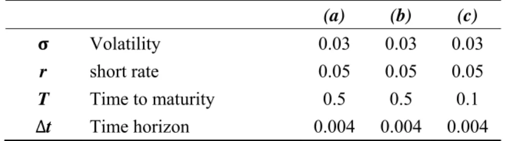
instruments based on ten correlated assets with all assets having an initial value of 100 and an annual volatility of 0.3. Table 1 describes the test portfolio in this paper. We assume 250 trading days in a year and a continuously compounded risk free rate of interest of 5%. For each case we investigate losses over 1 day (∆t=0.004 years) in Table 2. Table 3 is the covariance matrix we reference from Glasserman et al. (1999b).

Table 1 Portfolios

(a)Index

Loss over 1 day

Short 50 at-the-money calls and 50 at-the-money puts on 10 underlying assets, and all options have a maturity of 0.5 years. The covariance matrix for 10 asset prices is set to be the same as that in Glasserman, Heidelberger, and Shahabuddin [1999]. The initial asset prices are set as ( 100, 50, 20, 100, 80, 20, 50, 200, 150, 10)

(b)Index Loss over 1 day, Adjust

factor c1to -c1

Same as case (a), but we change the sign of the most important factor c1 partitioned by spectral decomposition in case (a) to –c1 in case (b) to generate the opposite relationship between portfolio loss L and Z1 for the purpose of comparison.

(c) ATM Delta-hedged Loss over 1 day

Short 10 at-the-money calls on each asset; all options have a maturity of 0.1 years, but with the numbers of puts on each asset increasing so that delta becomes 0, i.e., the portfolio is delta neutral. The initial asset prices are set as case (a).

Table 2 Parameter Settings

(a) (b) (c)

Volatility 0.03 0.03 0.03

r short rate 0.05 0.05 0.05

T Time to maturity 0.5 0.5 0.1

∆t Time horizon 0.004 0.004 0.004

(14)

0.289 0.069 0.008 0.069 0.084 0.085 0.081 0.052 0.075 0.114 0.069 0.116 0.020 0.061 0.036 0.088 0.102 0.070 0.005 0.102 0.008 0.020 0.022 0.013 0.009 0.016 0.019 0.016 0.010 0.017 0.069 0.061 0.013 0.079 0.035 0.090 0.090 0.051 0.031 0.075 0.084 0.036 0.009 0.035 0.067 0.055 0.049 0.029 0.022 0.062 0.085 0.088 0.016 0.090 0.055 0.147 0.125 0.073 0.016 0.112 0.081 0.102 0.019 0.090 0.049 0.125 0.158 0.087 0.016 0.127 0.052 0.070 0.016 0.051 0.029 0.073 0.087 0.077 0.014 0.084 0.075 0.005 0.010 0.031 0.022 0.016 0.016 0.014 0.143 0.033 0.114 0.102 0.017 0.075 0.062 0.112 0.127 0.084 0.033 0.176                                

In each case we first adjust the loss threshold b so that the probability to be estimated is close to 0.05, 0.01, and then we move to extreme large losses thresholds. We use two different methods—naïve Monte Carlo and the proposed IS algorithm. For purpose of comparing, we generate 1,000,000 simulation runs for the naïve Monte Carlo approach in each case, but only 5,000 simulation runs for proposed IS method. We report the result of estimating in Table 4, 5 and 6. We also summary the results of estimating ; in Table 7, 8 and 9.

5.1 Numerical Results of Value-at-Risk

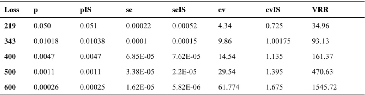
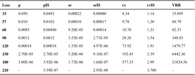
We report the point estimator of large loss for each portfolio in column 1. For each simulated result, we present the standard errors in parentheses. The results show that the IS estimator obtained from our algorithm is very close to the simulated ones in all cases considered compared with naïve Monte Carlo. In Tables 4, 5, and 6, we can see that coefficient of variation is near constant across a broad range of b by calculating upper-tail probability, . This indicates that the proposed estimator has bounded relative error and estimators with bounded relative error are the best class of importance sampling estimator (Heidelberger [1995]). The VRR ratio is significant over increasing thresholds of loss of each of the three testing portfolios.

Table 4 Simulated point estimator of portfolio (a)

Loss p pIS se seIS cv cvIS VRR

219 0.050 0.051 0.00022 0.00052 4.34 0.725 34.96 343 0.01018 0.01038 0.0001 0.00015 9.86 1.00175 93.13 400 0.0047 0.0047 6.85E-05 7.62E-05 14.54 1.135 161.37 500 0.0011 0.0011 3.38E-05 2.2E-05 29.54 1.395 470.63 600 0.00026 0.00025 1.62E-05 5.82E-06 61.774 1.675 1545.72

(15)

9

700 4.70E-05 5.11E-05 6.86E-06 1.43E-06 145.864 1.975 4624.53 800 9.00E-06 1.01E-05 3E-06 3.27E-07 333.3342 2.295 16788.023 900 3.00E-06 1.91E-06 1.73E-06 7.11E-08 577.35 2.63 118616.51

Table 5 Simulated point estimator of portfolio (b)

Loss P pIS se seIS cv cvIS VRR

219 0.050 0.050 0.00022 0.00048 4.35 0.68 40.71 343 0.0097 0.0099 9.82E-05 0.00013 10.080 0.93 113.19 400 0.0050 0.0051 7.08E-05 7.45E-05 14.057 1.029 180.45 500 0.0017 0.0018 4.16E-05 2.96E-05 24.00072 1.19 394.57 600 0.00057 0.00053 2.38E-05 1.04E-05 41.91 1.38 1055.54 700 0.00014 0.00014 1.19E-05 3.20E-06 83.91 1.58 2771.49 800 3.70E-05 3.37E-05 6.08E-06 8.66E-07 164.39 1.81 9871.33 900 7.00E-06 6.97E-06 2.65E-06 2.05E-07 377.96 2.077 33378.25

Table 6 Simulated point estimator of portfolio (c)

Loss p pIS se seIS cv cvIS VRR

33 0.050 0.0492 0.00022 0.00080 4.34 1.14 15.095 57 0.010 0.0102 0.00010 0.00017 9.78 1.20 68.79 60 0.0085 0.00840 9.20E-05 0.00014 10.78 1.21 82.53 90 0.0012 0.0012 3.53E-05 2.71E-05 28.26 1.54 340.83 120 0.00018 0.00018 1.35E-05 4.97E-06 73.92 1.91 1479.77 150 2.70E-05 2.70E-05 5.20E-06 9.16E-07 192.45 2.39 6442.36 180 3.00E-06 3.92E-06 1.73E-06 1.66E-07 577.35 2.99 21834.56 210 - 5.59E-07 - 2.93E-08 - 3.700 -

5.2 Numerical Results of Expected Shortfall

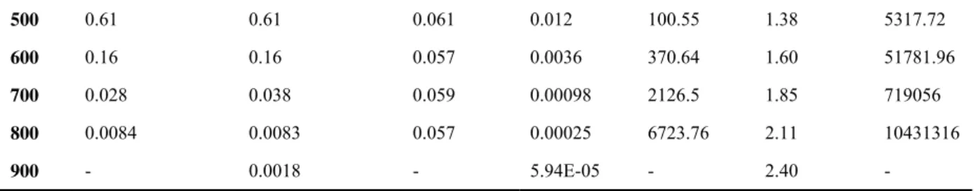
In Tables 7, 8, and 9, we report the results for the simulated upper-tail conditional mean, ; . We can see the point estimator is very close to naïve Monte Carlo apparently. The standard error of the proposed estimator is decreasing, and cv is constant, thus the estimator has bounded relative error in estimates of ; , and the VRR ratio is significant in each case.

Table 7 Simulated ; of portfolio (a)

Loss ; ; Se seIS cv cvIS VRR

219 14.9 14.8 0.073 0.18 4.91 0.84 34.18 343 4.26 4.19 0.067 0.064 15.83 1.070 225.17 400 2.18 2.17 0.065 0.035 30.018 1.16 681.56

(16)

500 0.61 0.61 0.061 0.012 100.55 1.38 5317.72 600 0.16 0.16 0.057 0.0036 370.64 1.60 51781.96

700 0.028 0.038 0.059 0.00098 2126.5 1.85 719056 800 0.0084 0.0083 0.057 0.00025 6723.76 2.11 10431316

900 - 0.0018 - 5.94E-05 - 2.40 -

Table 8 Simulated ; of portfolio (b)

Loss ; ; Se seIS cv cvIS VRR

219 14.94 12.09 0.073 0.125 4.94 0.73 68.90 343 4.22 4.27 0.069 0.062 16.42 1.040 243.6 400 2.21 2.21 0.067 0.035 30.44 1.14 700.99 500 0.64 0.63 0.063 0.012 98.56 1.41 5067.31 600 0.17 0.16 0.060 0.0038 346.73 1.67 49011.51 700 0.035 0.038 0.065 0.00107 1820.21 1.96 729839.3 800 0.0079 0.0086 0.039 0.00028 4963.21 2.32 3806620 900 0.0027 0.0018 0.016 6.77E-05 6122.23 2.62 12437606

Table 9 Simulated ; of portfolio (c)

Loss ; ; se seIS cv cvIS VRR

33 2.43 2.86 0.015 0.19 6.37 4.89 1.21 57 0.75 0.74 0.015 0.013 20.68 1.30 258.60 60 0.64 0.64 0.015 0.011 24.015 1.28 359.02 90 0.13 0.13 0.015 0.0029 114.89 1.62 5160.82 120 0.024 0.025 0.014 0.00066 584.89 1.91 92997.65 150 0.0044 0.0044 0.010 0.00016 2319.28 2.52 816072.6 180 0.00054 0.00076 0.0029 3.07E-05 5378.042 2.85 1849151 210 - 0.00013 - 7.14E-06 - 3.99 -

6. CONCLUDES

This paper analyzed and experimented with an importance sampling technique for estimates of value-at-risk and expected shortfall by approximating the portfolio loss using simulated upper-tail probability, and simulated conditional mean of a portfolio loss, ; . First we apply spectral decomposition to the covariance matrix of underlying risk factors to decide the key factor (c1) in relation to the correlated underlying risk factors. Then we propose a two-step procedure to generate

X. We can sample random variates Z first and then find Z1. Given simulated loss value of the option portfolio driven byZ , portfolio loss L is a strictly monotonic

(17)

11

function in relation to Z1. Based on the different relationships, an importance sampling change of measure can then be determined by solving Z1. The method was applied to option portfolios with different characteristics that can prove its efficiency. Our numerical results show that the derived VaR and expected shortfall are very close to the naïve Monte Carlo method in all cases considered, and produces large variance reductions; more than two orders of magnitude and often more than three orders of magnitude improvements are obtained, which demonstrate dramatic variance reduction for extreme portfolio loss. Our algorithm shows that the proposed estimator has constant coefficient of variation, which suggests the proposed estimator has bounded relative error.

Under our framework, in practical all parameters necessary for pricing of the instrument and measuring the VaR and expected shortfall are available from the trading and valuation system at the front office in a financial institution. The nature of our algorithm is straightforward and easy for realizing the practical needs of risk management. Therefore, we conclude our algorithm is an efficient vehicle for measuring the option portfolio loss.

7. REFERENCES

1. Acerbi, C. and D. Tasche. "On the Coherence of Expected Shortfall." Journal of Banking and Finance, 26 (2002), pp. 1487-1503.

2. Alexander, C. Market Risk Analysis, value-at-risk Models: Wiley 2009.

3. Artzner, P., F. Delbaen, J. M. Eber, et al. "Think Coherently." Risk, 10 (1997), pp. 68-71.

4. Artzner, P., F. Delbaen, J. M. Eber, et al. "Coherent Measure of Risk." Mathematical Finance, 9 (1999), pp. 203-228.

5. Basel Committee on Banking Supervision. Amendment to the capital accord to incorporate market risks, 1996. Available from http://www.bis.org (accessed November 2011).

6. Asmussen, S. and P. Glynn. Stochastic Simulation: Algorithms and Analysis: Springer 2007.

7. Chen, Z. and P. Glasserman. "Fast pricing of basket default swaps." Operations Research Proceedings 2005, 56, 2 (2008), pp. 286-303.

8. Chiang, M.-H., M.-L. Yueh and M.-H. Hsieh. "An efficient algorithm for basket default swap valuation." The Journal of Derivatives, 15, 2 (2007), pp. 8-19. 9. Glasserman, P., P. Heidelberger and P. Shahabuddin. "Asymptotically optimal

importance sampling and stratification for pricing path-dependent options." Mathematical Finance, 9 (1999a), pp. 117-152.

(18)

10. Glasserman, P., P. Heidelberger and P. Shahabuddin. Importance Sampling and Stratification for Value-at-Risk. Proceedings of the Sixth International Conference Computational Finance, In Y.S. Abu Mostafa, B. LeBaron, A.W. Lo, A.S.

Weigend, eds., MIT Press, 1999b.

11. Glasserman, P., P. Heidelberger and P. Shahabuddin. "Variance reduction techniques for estimating value-at-risk." Management Science, 46 (2000), pp. 1349-1364.

12. Glasserman, P., P. Heidelberger and P. Shahabuddin. "Portfolio Value-At-Risk with Heavy-Tailed Risk Factors." Mathematical Finance, 12 (2002), pp. 239-269. 13. Glasserman, P. and Y. Wang. "Counterexamples in importance sampling for rare

event probabilities." The Annals of Applied Probability, 7 (1997), pp. 731-746. 14. Heidelberger, P. "Fast simulation of rare events in queueing and reliability

models." ACM Trans. Model. Comput. Simul., 5, 1 (1995), pp. 43-85.

15. Jorion, P. value-at-risk: The New Benchmark for Controlling Derivatives Risk, New York: McGraw-Hill 1997.

16. Joshi, M. and D. Kainth. "Rapid and accurate development of prices and Greeks for nth to default credit swaps in the Li model." Quantitative Finance, 4, 3 (2004), pp. 266-275.

17. RiskMetrics Technical Document, Morgan, J. P., 1996.

18. Rouvinez, C. "Going Greek with VAR." Risk, 10, 2 (1997), pp. 57-65. 19. Wilson, T. value-at-risk, Wiley, Chichester, England 1999.

20. Yueh, M.-L. and M. C. W. Wong. "Analytical VaR and Expected Shortfall for Quadratic Portfolios." Journal of Derivatives, 2010, 1 (2010), pp. 1-12.

(19)

ge 國科會補助專題研究計畫項下出席國際學術會議心得報告 日期： 2012 年 1 月 30 日 一、參加會議經過國際長壽風險與資本市場解決方案研討會是國際級的年會，會議的參與者包括產業界、學術界的專家學者等實際負責政策的決策者，為提升政大風管的國際能見度、並與國際級學者交換研究心得，此次我與風管系老師共同參加此研討會，並合作發表研究論文，並藉由聆聽其它學者的發表及心得，來了解目前長壽風險領域最新的研究情況；同時也可以透過在場與會學者先進對我們論文的問題與意見，利用腦力激盪的方式尋找各種可能的未來的研究方向與建議。研討會的地點在法國法蘭克福，此次會議的重點主題即是強調將長壽風險視為可做為投資者利用的資產的相關研究，與我們發表的論文主題「使用保單折現進行保險公司之死亡風險避險：資產負債管理方法」相當貼近，因此在場有相當多的學者與我們的研究相當感興趣，有不少學者對於保單貼現的在台灣的普及程度與保險公司與於長壽風險的態度與管理現況。計畫編號 NSC 99-2410-H-004-086 計畫名稱投資組合信用風險，投資組合市場風險與路徑相依選擇權評價之快速蒙地卡羅演算法研究出國人員姓名謝明華服務機構及職稱國立政治大學風險管理與保險學系會議時間 2011 年 9 月 8 日至 2011 年 9 月 9 日會議地點

Goethe University Frankfurt, France.

會議名稱

(中文)第七次國際長壽風險管理與資本市場解決方案研討會

(英文) Longevity 7: Seventh International Longevity Risk and

Capital Markets Solutions Conference

發表論文題目

(中文)使用保單折現進行保險公司之死亡風險避險：資產負債管理方法

(英文) Using Life Settlements to Hedge the Mortality Risk of the Life Insurers: An Asset-Liability Management Approach"

(20)

二、與會心得

在session 1主要是討論風險管理的議題，我聆聽了Elisa Luciano、Luca Regisz、與Elena Vignar共同研究發表的「Delta and Gamma Hedging of Mortality and Interest Rate Risk」，這篇論文研究年金現金流量的避險問題，並假設死亡率與利率均為隨機過程，他們使用delta-gamma的避險技術來處理死亡風險，並藉由分析模擬風險因子的變化，來了解年金的價值變化。

在第Session 2，則是由我和政大風管系老師共同發表「Using Life Settlements to Hedge the Mortality Risk of the Life Insurers: An Asset-Liability Management Approach」，我們提出一個基於避險方法基礎，以評估保單貼現避險效率的研究方法，來分析保險公司保單貼現商品對於死亡風險避險的效果，我們的數值方法證明保險公司可以有效的利用保單貼現來處理死亡風險，這篇論文使用保單貼現做為避險工具是較為先進的做法，也因此引起與會的學者不少互動，對於本研究未來的發展有相當的助益。

在session 3我則選擇聆聽由Rui Zhou，Johnny Siu-Hang Liy，Ken Seng Tan共同發表的「A Two-Population Mortality Model with Transitory Jump Effects」，這篇論文討論死亡率的動態隨機過程存在著跳躍＂jump＂的影響，這些jump會顯著的影響連結死亡率的證券價格，因此也必須在模型中考量。這篇論文強調過去的模型均僅考量單一族群基差風險，因此在不同族群間的模型適用性未曾有過研究探討，這篇論文提出兩個版本的模型來分析這些不同族群之間的jumps規則，對於模型的假設等有不少值得深入了解的地方，我也提出問題與一些模型上的建議予發表論文的學者共同討論。三、考察參觀活動(無是項活動者略) 無四、建議無五、攜回資料名稱及內容 (1) 大會議程 (2) 大會論文集光碟六、其他無

(21)

國科會補助計畫衍生研發成果推廣資料表

日期:2012/01/09

國科會補助計畫

計畫名稱: 投資組合信用風險，投資組合市場風險與路徑相依選擇權評價之快速蒙地卡羅演算法研究計畫主持人: 謝明華計畫編號: 99-2410-H-004-086- 學門領域: 財務

無研發成果推廣資料

(22)

99 年度專題研究計畫研究成果彙整表

計畫主持人：謝明華計畫編號： 99-2410-H-004-086-計畫名稱：投資組合信用風險，投資組合市場風險與路徑相依選擇權評價之快速蒙地卡羅演算法研究量化成果項目實際已達成數（被接受或已發表）預期總達成數(含實際已達成數) 本計畫實際貢獻百分比單位備註（質化說明：如數個計畫共同成果、成果列為該期刊之封面故事 ... 等）期刊論文 0 0 100% 研究報告/技術報告 0 0 100% 研討會論文 0 0 100% 篇論文著作專書 0 0 100% 申請中件數 0 0 100% 專利已獲得件數 0 0 100% 件件數 0 0 100% 件技術移轉權利金 0 0 100% 千元碩士生 0 0 100% 博士生 0 0 100% 博士後研究員 0 0 100% 國內參與計畫人力（本國籍）專任助理 0 0 100% 人次期刊論文 0 2 100% 研究報告/技術報告 0 0 100% 研討會論文 0 0 100% 篇論文著作專書 0 0 100% 章/本申請中件數 0 0 100% 專利已獲得件數 0 0 100% 件件數 0 0 100% 件技術移轉權利金 0 0 100% 千元碩士生 0 0 100% 博士生 0 2 100% 博士後研究員 0 0 100% 國外參與計畫人力（外國籍）專任助理 0 0 100% 人次

(23)

其他成果

(

無法以量化表達之成果如辦理學術活動、獲得獎項、重要國際合作、研究成果國際影響力及其他協助產業技術發展之具體效益事項等，請以文字敘述填列。) 預計發表於國際期刊之撰寫中的 Working Paper：

1. Hsieh, Ming-hua, Liao, Wei-cheng, Chen, Chung-lung A Fast Algorithm for Estimating

Value-at-Risk and Expected Shortfall, Working Paper, 2011.

2. Hsieh Ming-hua, So-de Shyu, Yi-Hsi Lee, and Yu-Fen Chiu Fast simulation of portfolio credit

risk under general multifactor copula models, Working Paper, 2011.

成果項目量化 名稱或內容性質簡述 測驗工具(含質性與量性) 0 課程/模組 0 電腦及網路系統或工具 0 教材 0 舉辦之活動/競賽 0 研討會/工作坊 0 電子報、網站 0 科教處計畫加填項目計畫成果推廣之參與（閱聽）人數 0

(24)

國科會補助專題研究計畫成果報告自評表

請就研究內容與原計畫相符程度、達成預期目標情況、研究成果之學術或應用價

值（簡要敘述成果所代表之意義、價值、影響或進一步發展之可能性）

、是否適

合在學術期刊發表或申請專利、主要發現或其他有關價值等，作一綜合評估。

1. 請就研究內容與原計畫相符程度、達成預期目標情況作一綜合評估

■達成目標

□未達成目標（請說明，以 100 字為限）

□實驗失敗

□因故實驗中斷

□其他原因

說明：

2. 研究成果在學術期刊發表或申請專利等情形：

論文：□已發表 □未發表之文稿 ■撰寫中 □無

專利：□已獲得 □申請中 ■無

技轉：□已技轉 □洽談中 ■無

其他：（以 100 字為限）

3. 請依學術成就、技術創新、社會影響等方面，評估研究成果之學術或應用價

值（簡要敘述成果所代表之意義、價值、影響或進一步發展之可能性）（以

500 字為限）

This project analyzed and experimented with an importance sampling technique for estimates of value-at-risk and expected shortfall by approximating the portfolio loss using simulated upper-tail probability, P(L>b) and simulated conditional mean of a portfolio loss, E[L；L>b]. First we apply spectral decomposition to the covariance matrix of underlying risk factors to decide the key factor (c1) in relation to the correlated underlying risk factors. Then we propose a two-step procedure to generate X. We can sample random variates first and then find Z1. Given simulated loss value of the option portfolio driven by , portfolio loss L is a strictly monotonic function in relation to Z1. Based on the different relationships, an importance sampling change of measure can then be determined by solving Z1. The method was applied to option portfolios with different characteristics that can prove its efficiency.

Our numerical results show that the derived VaR and expected shortfall are very close to the na&iuml；ve Monte Carlo method in all cases considered, and produces large variance reductions； more than two orders of magnitude and often more than three orders of magnitude improvements are obtained, which demonstrate dramatic variance reduction for extreme portfolio loss. Our algorithm shows that the

(25)

proposed estimator has bounded relative error.

Under our framework, in practical all parameters necessary for pricing of the instrument and measuring the VaR and expected shortfall are available from the trading and valuation system at the front office in a financial institution. The nature of our algorithm is straightforward and easy for realizing the practical needs of risk management. Therefore, we conclude our algorithm is an efficient vehicle for measuring the option portfolio loss.

投資組合信用風險、投資組合市場風險與路徑相依選擇權評價之快速蒙地卡羅演算法研究

行政院國家科學委員會專題研究計畫 成果報告