國
立
交
通
大
學
網路工程研究所
碩
士
論
文
真實網路流量分類演算法:
利用封包大小分佈與連接埠關聯性之流量辨識
Application Classification in Real Traffic:
Using Packet Size Distribution and Ports Association
研 究 生:彭偉豪
指導教授:林盈達 教授
中 華 民 國 九 十 六 年 六 月
II
真實網路流量分類演算法:
利用封包分佈與連接埠關聯性之流量辨識
Application Classification in Real Traffic:
Using Packet Size Distribution and Ports Association
研 究 生:彭偉豪 Student: Wei-Hao Peng
指導教授:林盈達 Advisor: Dr. Ying-Dar Lin
國立交通大學
網路工程研究所
碩士論文
A Thesis
Submitted to Institutes of Network Engineering College of Computer Science
National Chiao Tung University in partial Fulfillment of the Requirements
for the Degree of Master
In
Computer Science and Engineering
June 2007
HsinChu, Taiwan, Republic of China
III
真實流量分類演算法:
利用封包分佈與連接埠關聯性之流量辨識
學生: 彭偉豪
指導教授: 林盈達
國立交通大學網路工程研究所
摘要
傳統的藉由封包特徵來辨識流量的方法已經使用了很長的一段時間,但是遇 到應用程式使用加密通訊協定的狀況下便無法使用。相關的研究中發現可以從應 用程式在網路傳輸層中展現的特性作為可被辨識的依據。這類方法可分為網路中 主機的社交關係與行為統計兩大類型,但是其方法卻有準度不足或是辨識耗時而 無法在即時的網路環境中運用。本篇提出了使用應用程式在傳輸層中的封包大小 分布特徵加上埠關聯特性的辨識方法。在真實流量中的每條連線皆會經由特徵值 運算後變成多維空間中的一個向量,並且藉由計算先前分析出的各應用程式在空 間中的代表點之差異即可辨識出該連線屬於何種應用程式,若在加上利用埠關聯 之特性,對於應用程式連線的辨識正確率平均可高達 96%以上,且擁有平均 4% 的 誤判率及 5% 的漏判率,這樣的誤判主要發生於即時通訊軟體中。最後,我們提 出一個簡單的即時的線上架構,證明我們的方法平均可以在一百到三百個封包內 辨識出一條連線,且可用於線上的閘道器中。 關鍵字: 流量辨識、傳輸層行為、封包大小分佈、埠關聯、點對點IV
Application Classification in Real Traffic:
Using Packet Size Distribution and Ports Association
Student: Wei-Hao Peng
Advisor: Dr. Ying-Dar Lin
Department of Computer Science and Engineering
National Chiao Tung University
Abstract
Signature based classification methodology has been used for a long time, but it can't be applied to encrypted protocol message. Some researches try to find out useful characteristics of separate applications from their transport layer behaviors that can be divided into two kinds: social network behaviors and statistical behaviors. Most of them are time-consuming due to a huge amount of information needed. In our work, we use Packet Size Distribution and Ports Association to achieve our goal. Every succeeded connection would be transformed into one vector in the multi-dimensional coordinate spaces and classified into some specified application or other unknown ones. Besides, the Euclidean distances of every connection between all individual centers, the representatives of the applications, will also be computed. Once a connection is identified and classified into some certain session, we can use ports association algorithm to associate and accelerate other connections in the same session. Using the proposed method, we can reach high classification accuracy rate, 96% on average, and low false positive and false negative rate, 4%~5%, after the preparation process of 100~200 packets. Lastly, we present an basic on-line architecture to show the correctness and simplicity.
Keywords: Traffic classification, Transport layer behaviors, Packet size distribution,
V
Contents
Chapter 1. Introduction ... 1
Chapter 2. Observing and Characterizing Application Flow Behaviors. ... 4
2.1 Description of experiment environment ... 4
2.2 Dominating Sizes (DS) and its’ proportion (DSP) ... 7
2.3 Change Cycle ... 8
2.4 Centralized Dominating Size ... 9
2.5 Ports Locality ... 10
2.6 Example of calculating metrics ... 10
Chapter 3. Euclidean Distance Clustering Algorithm ... 12
3.1 Introduction to the classification methodology ... 12
3.2 Transform connections into vectors in spaces ... 12
3.3 Center Training ... 13
3.4 Association of connections to an application ... 14
3.5 Session association by ports association ... 15
Chapter 4. Evaluation ... 18
4.1 Evaluation Environment ... 18
4.2 Connection Recognition Rate(CR) and Accuracy ... 19
4.3 False positive rate and False negative rate ... 21
4.4 On-Line Gateway Architecture analysis ... 22
Chapter 5. Conclusions and Future work ... 25
Reference ... 26
VI
List of Figures
Figure 1 Pure Lab Traffic Analyzing Environment. ... 5
Figure 2 Packet size distribution of each application ... 5
Figure 3. Same application has similar PSD ... 6
Figure 4. Different Applications have different PSD ... 7
Figure 5. Algorithm of how to calculate change cycle of a PSD ... 9
Figure 6. eMule PSD of a sample from packet 1 to 50 ... 11
Figure 7. 2 phases classification methodology. ... 12
Figure 8. Algorithm of connection recognition ... 14
Figure 9. Algorithm of session association using PAT ... 15
Figure 10. The whole classification algorithm flow ... 16
Figure 11. Connection recognition rate ... 19
Figure 12. Accuracy for session detection ... 21
VII
List of Tables
Table 1: Applications used in this work. ... 4
Table 2: The average numerical results of five metrics for each application. ... 7
Table 3. Connections in the collectedtraffic. ... 18
Table 4: False positive/negative rate of each application. ... 21
1
Chapter 1. Introduction
Classifying traffic flows according to the applications behaviors is essential to real traffic analysis. The Internet service providers can design the network and determine the management policy from the statistics of application protocols. Therefore, traffic identification and classification are the basis of traffic analyzing research, especially for network intrusion detection mechanisms.. Network intrusion detection relies on the classification to help extracting high-level semantic context from traffic.
Traditional classification methodology based on identifying packet payload signatures and their related port numbers was effective[1,2], but this kind of method is no longer works as well with growing P2P traffic, which intends to disguise themselves. Because many non-standard P2P protocols exist, and most of them are using payload encryption and port randomization, the difficulty in classification gets even higher. Therefore, it is impatient to find new characteristics other than packet payload information.
By the reasons above, we start to find application characteristics without information in payload. Previous works have shown that classification methods using transport-layer behavior of applications have been proposed in the literature. They can be categorized into two classes: (i) Statistical properties, which use flow statistical analysis to classify network traffic or at least describe the behaviors. [3, 4, 5] This approach employs the information of packet sizes, packet inter-arrival time and packet arrival order to determine which classes of application that the traffic belongs to, such as interactive, bulk transfer and streaming or transactional ones. (ii) Socialized network behaviors, which the first one proposed by T. Karagiannis et al. is observing connection patterns between source and destination IP pairs, then examining the flow history to reveal the different parts of P2P protocols [6, 7]. Later,
2
he proposed a new method called BlinC which is a topology-based classification method that associates Internet hosts with applications into three socialized levels, and used the difference between these levels as characteristics to classify the flows [8]. These approaches can provide rich informationand give the highly accurate results at the expense of complex analysis. However, it has low performance and cannot be applied to an on-line architecture.
In this paper, we propose a novel approach to classify traffic flows, which based on the characteristics of packet size distribution (PSD) per application flow. And use port locality per session of an application to associate the connections. There may be one or lots packets in one connection. We characterize the PSD of connections as vectors in a multi-dimensional vector space.. The entries of a vector are defined as following: (1) Change Cycle (CC), to represents if the PSD of a flow changes dramatically. In general, it always happens to P2P or streaming protocols, (2)
Dominating Sizes (DS), to represents the sizes that appear most frequent in a flow, (3) Dominating Sizes Proportion (DSP) and (4) Variance of Dominating Sizes. In the first
phase of our method, we locate the representative centers of the specialized applications. In the second one, we use our clustering algorithm to classify the vectors of all connections into applications.
The proposed classification provides a fast, accurate and could be applied into on-line architecture with features we defined in our work. First, we define the features of applications without the payload information. The algorithm is based on PSD and does not have to access any payload patterns as information for classification. This approach can work even when the traffic is encrypted. Second, different applications have different types of PSD. For example, the PSD of P2P applications vary violently but the PSD of Http or FTP ones is even smooth. Third, our approach can classify traffic in a very short time, say hundreds of packets and still have high accuracy, say
3
up to 90%. Last, unknown applications could also be classified. According to the vectors of all connections, we can determine what applications those connections belong to. If one connection is not classified into some application in the end, we divide it into unknown ones.
This paper is organized as follows. Chapter 2 describes the experimental environment and the characteristics we found in packet size distribution. In Chapter 3, we proposed the new classification algorithm using the features in Chapter 2. We evaluate the accuracy and performance of the algorithm in Chapter 4 and give a simple on-line architecture. Then we conclude this work and discuss the results with different background traffic as future works.
4
Chapter 2. Observing and Characterizing Application Flow
Behaviors.
2.1 Description of experiment environment
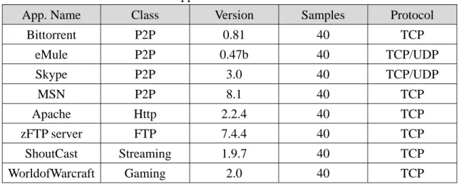
In our traces, it is necessary to collect pure traffic of applications to analyze the transport layer behaviors of those applications. We construct an In-Lab Pure Traffic Recording Environment over Ethernet as figure 1 shows, to dump pure application traffic samples by using Netlimitter v2.0 [9], which is one kind of traffic management software used to restrict which application in a host can build connections to other hosts. Next to Netlimitter, we run the program and then use Wireshark [10] to dump traffic for four different situations: (1) time duration, there are 30 seconds, 5 minutes, and the whole session respectively; (2) data sources, for those file-sharing applications, we give different file sources to collect traffic; (3) host loading; this information is used to show that no matter how high the host loading is, the PSD of application wouldn’t be affected; (4) application settings; our purpose is to observe that whether or not the PSD of application would be affected by the bandwidth settings, quality settings, or encrypted protocol settings. Table 1 shows applications and its’ corresponding version we used in our research and the number of traffic samples we collect.
Table 1: Applications used in this work.
App. Name Class Version Samples Protocol
Bittorrent P2P 0.81 40 TCP eMule P2P 0.47b 40 TCP/UDP Skype P2P 3.0 40 TCP/UDP MSN P2P 8.1 40 TCP Apache Http 2.2.4 40 TCP zFTP server FTP 7.4.4 40 TCP ShoutCast Streaming 1.9.7 40 TCP WorldofWarcraft Gaming 2.0 40 TCP
5
Figure 1: In-Lab Pure Traffic Recording Environment.
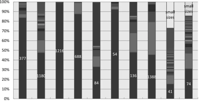
Figure 2: Packet size distribution of each application.
Each PSD of an application could be obtained from all of its’ own connections. We compute size information of one connection from IP level and ignore connections which do not belong to TCP or UDP protocols. According to our observations from dumped traffic, the PSD graph of applications is shown in figure 2. Cross axle means each application in our experiment, the other axle means its’ size proportion. The small sizes inside the figure mean that the proportions of these sizes are too small to represent them in the figure. We find PSD of applications have features such like (1)Same application has several similar PSDs, as shown in figure 3, (2)Different applications have different PSDs, as shown in figure 4, which the cross axle means
377 1180 1216 688 84 54 136 1388 41 74 small sizes small sizes 0% 10% 20% 30% 40% 50% 60% 70% 80% 90% 100%
6
packet sequence and vertical axle means packet size that correspond to the sequence. (3)PSDs of P2P and streaming applications vary more dramatically. We believe that the reason is because of the different sizes of data structure from distinct implementation of applications to the kernel buffer size. Therefore, the packed packet sizes are also different between applications. From the point of view, the variation of packet size could be a good feature to classify applications. In this work, we use five metrics to represent each PSD of the applications, and the corresponding values are shown in Table2.
Bittorrent sample1 Bittorrent sample 2 Figure 3: Same application has similar PSD.
7
zFTP server(Ftp) Apache (Http) Figure 4: Different applications have different PSD.
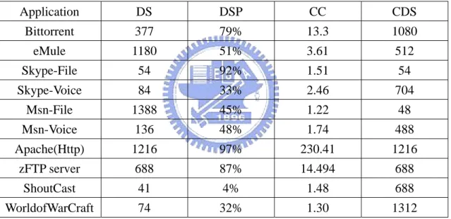
Table 2: The average numerical results of five metrics for each application.
Application DS DSP CC CDS Bittorrent 377 79% 13.3 1080 eMule 1180 51% 3.61 512 Skype-File 54 92% 1.51 54 Skype-Voice 84 33% 2.46 704 Msn-File 1388 45% 1.22 48 Msn-Voice 136 48% 1.74 488 Apache(Http) 1216 97% 230.41 1216 zFTP server 688 87% 14.494 688 ShoutCast 41 4% 1.48 688 WorldofWarCraft 74 32% 1.30 1312
2.2 Dominating Sizes (DS) and its’ proportion (DSP)
Every PSD graph represents the size distribution information of a connection. In addition to the well-known full payload (1500 bytes) and acked packet (40 bytes), there are other various sizes in PSD. We pay our attention to those packets with bigger proportion in a connection. We named these packet sizes as “Dominating Sizes” (DS) of a connection. In our experiment, each application has quite different dominating sizes and the dominating size proportions (DSP). DS and DSP are computed as follows: Assume there are x sizes in one PSD of a connection, say
8 ⎪ ⎪ ⎪ ⎩ ⎪⎪ ⎪ ⎨ ⎧ = ) ( ) ( ) ( ) ( 3 3 2 2 1 1 x x pro P P P pro P P pro P P pro P P M M (1)
Where Pi means the i-th size, pro(Pi) means the proportion of Pi, and
pro(Pi-1)≥pro( Pi), ∀i = 1~x.
1. Define a Bound such that the Dominating Sizes vector will be
}, ,..., , , {P1 P2 P3 Pn DS = ∀Pj ∈DS,Pj ∈P (2) where Pj is the first size such that
∑
= > j n n bound p pro ~ 1 )
( , and the bound is set to
90% by default.
3. The DSP = {pro(P1), pro(P2), … , pro(Pj)}.
From the calculation, by assumption of all above, we also find every proportion of dominating size has almost a fixed range of variation for each application.
2.3 Change Cycle
From the analysis of PSD graph, the size variation of P2P and streaming protocols are very dramatic than other applications. Since P2P and streaming protocols are various and different. It is helpful to decide what applications a connection is belonged to by quantifying this size variation. We called it as “Change Cycle” of a PSD.
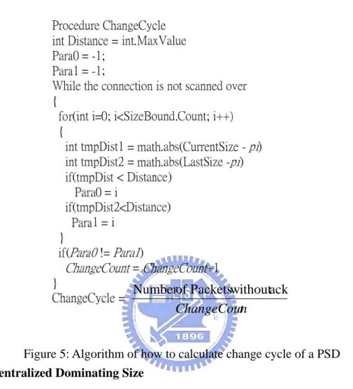
By equation (1), every PSD has its’ size bound DS. We define a “size bound change” which is a size variation from one size bound in P to another. The distance of every packet but without acked packets would be calculated between every Pi in DS. What size bound that a packet belonged to is decided by the shortest distance between them. Then a change cycle of a PSD is defined by the average number of packets
9
that a size bound change happens. Figure 5 shows the algorithm that describes how to calculate the change cycle.
t ChangeCoun ack without Packets of Number
Figure 5: Algorithm of how to calculate change cycle of a PSD
2.4 Centralized Dominating Size
In addition to the size variation, we also analyze the status of size distribution degree of size distribution and use variance of size that based on the expected value of PSD and dominating size. By the equation (2), we can define a equation that represents what size of dominating sizes that all sizes in equation (1) are closest to it. We call it as the Centralized Dominating Size(CDS), as equation (3)
DS P P pro P P CDS i i DS n i i DS i − ∀ ∈ =
∑
= , )} ( * ) ( min{ 1 2 , (3)The CDS provides a way to describe that which dominating size are closest to the most of all packet sizes in size distribution. Table 2 lists a comparison between CDS
10
and Main Dominating Size (MDS), which means the dominating size in DS that has the largest proportion.
CDS of a PSD would help us to describe the status of size distribution of a connection. Also, it can represent size distribution behaviors of an application, especially for P2P/streaming services and Skype voice chat..
2.5 Ports Locality
In IPv4 structure, every host has 65536 ports to use. In general, when a session of an application needs to build multi-connections, kernel assigns continuous ports range for every application, even for applications using randomized port numbers. Once some port number is binded to the first connection, the remainder connections will use continuous port numbers. This feature is not willing to use for signature based classification methodology. The reason is because it only needs to verify a few bytes in packet payloads to make a decision. For the method utilizing the transport layer behaviors, the feature will be very useful if a connection is recognized to a specific application, the port information can be used for associating other connections. The details of how to use this feature is described in section 3.3.
W conn In th 3.33 we info We’ll then g nection. Fig his sample, 3. The reaso analyzed ormation. Figure give a simp gure 6 show we have D on why the is because 6: eMule PS lified exam ws the PSD DS = {1180, change cyc this simp 11 SD of a sam mple that ho of fifty pac , 410, 730}, cle of this P plified samp mple from p ow to calcul ckets of an , DSP = {56 PSD is not ple is too packet 1 to 5 late metrics eMule conn 6%, 18%, 1 close to the short to 50 s of an eMu nection sam 18%} and C e original v collect eno ule’s mple. CC = value ough
12
Chapter 3. Euclidean Distance Clustering Algorithm
3.1 Introduction to the classification methodology
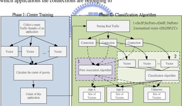
In the classification methodology we proposed, every connection in real traffic will be transformed to a vector in a multi-dimensional vector space. And each application implementation will have a vector to represent it. The whole methodology flow can be divided into 2 phases as Figure 7. The first phase is to decide the cluster centers for the applications. The second one parses all the connections in real traffic into vectors, and compares entries in Ports Association Table (PAT). If the corresponding pairs <SrcIP, SrcPort>, <DstIP, DstPort> do not appear in PAT, we would compute the Euclidean distances between the vectors and all the cluster centers and then decide which applications the connections are belonging to
Collect a many Traffic Samples of an
application
Vector Vector Vector
Calculate the center of gravity
Center of this application
Parsing Real Traffic
Connection Connection Connection
...
...
Ports Association Algorithm
App A App B Unknown
Vector Vector ... Vector
Classification Algorithm Sets of Vectors Sets of Vectors Sets of Vectors 1:<SrcIP,SrcPort>,<DstIP, DstPort> 2:normalized vector <DS,DSP,CC>
Figure 7: Two phases of classification methodology.
3.2 Transform connections into vectors in spaces
Four metrics are defined in Chapter 2: Dominating Sizes (DS), Proportions of
Dominating Sizes (DSP), Size Bound Count (SBC), and Change Cycle (CC). Every
13
in the vector are not in the same standard, it’s better to normalize them in the same range, say 0~1, for the purpose of balancing the weight of each entry. The normalization equation of each entry is as follows:
Size Max Frame _DS DS normalized = , (5) DSP DSP normalized_ = , (6) CC CC normalized _ = 1 , (7)
Besides, in our traces, we find that well-known protocol applications, such as apache server and zFTP server, and P2P applications such as Bittorrent and eMule have less number of SBCs. Streaming applications have a large number of SBCs. Therefore, we can separate well-known protocol applications and P2P/Streaming applications into the different vector spaces. And streaming applications will be separated in another one. We will automatically expand the lower dimensional vector to have an identical dimension to the higher one in the following vector operations.
3.3 Center Training
In this phase, our experiment collects 50 pure traffic samples for each application. Assume the vectors of all connections for an application Ai’s 50 samples are V = {v1,
v2,…, vk}. Then the center of Ai is defined as v V
k v C i k i i i = ∀ ∈
∑
= , 1 .The accuracy of our algorithm depends on choosing the appropriate application samples. For those applications that have various implementations on different platforms, it is necessary to choose the most famous ones to calculate their metrics as centers. For example, eMule client (http://www.eMule-Project.net) has windows and Linux based editions, and the official site always supplies the newest version, that is, 0.47c. The statistical analysis reveals that the 0.47c windows version on
14
SourceForge.net (http://sourceforge.net/) has 15,000 downloads in average for each day, and is the most popular implementation of eMule clients. So, the 0.47c windows version would be the best choice to calculate eMule’s center.
We also find that different implementation of application may have different center. Like eMule, which we mentioned above, the Windows version and Linux version have really different center.
3.4 Association of connections to an application
Figure 8: Algorithm of connection classification.
In the classification stage, the Euclidean distance (E_Dist) between two vectors is defined as 2 2 1 2 1 2 1, ) ( , ) ( ) (
_Dist Dist DS DS Dist DSP DSP CC CC
E = + + −
, (8)
where Dist(A,B) is the Euclidean distance between two same dimensional vectors A and B. Since vectors of the same application are quite similar, the Euclidean distance between the vectors of an application would be short. A connection is claimed to belong to a certain application if it has the shortest distance to the center of that
15 application.
The false positives may occur when an application’s center is not in our defined space. This case may exist in real traffic analysis, and if we use the algorithm to recognize it, those connections will be recognized as other applications. A simple way to address this problem is to find as many application centers as possible, but the effectiveness to reduce false positives is not guaranteed. From the analysis of our experiment, we define a threshold range for each center. If a vector Vi is calculated
and decided belonging to certain center Ci by the classification methodology, it’s DS
compared to Ci’s DS exceeds ± 50 bytes, and DSP exceeded ± 20%. , and then this
connection should belong to a certain unknown application instead. And it would also be classified into the unknown class. The entire connection recognition algorithm is as Figure 8. The function of transform function for connection is to extract this connection’s metric tuples.
3.5 Session association by ports association
Figure 9: Algorithm of session association using PAT
16
The PSDs of the same application may be different due to the variety of the implementation. Hence false negatives may occur in our classification algorithm. To solve this problem, we propose a method called “Ports Association” by using the port locality described in chapter 2. Once a connection is recognized to be from some application’s session, we could obtain a 4-tuple pair <SrcIP, SrcPort, DstIP, DstPort>, which means the two hosts run an instance of certain implementation of application with SrcPort and DstPort. These information will be recorded in the Ports Association
Table (PAT) with the form <SrcIP, SrcPort, AppName> and <DstIP, DstPort,
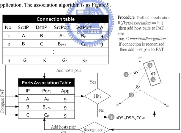
AppName>. For other connections, if one of their hosts is already in the PAT, and the port number in the pair <SrcIP, SrcPort> or <DstIP, DstPort> is continuous compared with one entry of PAT. We can say this connection belongs to the same session of one application. The association algorithm is as Figure 9.
Ports Association Table IP Port App A Ap 9 B Bp+1 9 C Cp 9 Connection table
No. SrcIP DstIP SrcPort DstPort A
1 A B Ap Bp 9 2 B C Bp+1 Cp 9 … n G K Gp Kp <DS1,DSP1,CC1> 1 1 7 8 9
Figure 10: The whole classification algorithm flow
The whole classification algorithm is organized in two steps: Every connection in the connection table will first run the Port Association algorithm. If the result is hit,
17
the connection would belongs to a certain application, and its’ SrcPair, DstPair will be added to the PAT. If not, the connection will run the Connection Recognition algorithm to classify the connection. The host pair of recognized connection will then also be added to PAT. The complete classification algorithm is shown in Figure 10.
18
Chapter 4. Evaluation
4.1 Evaluation Environment
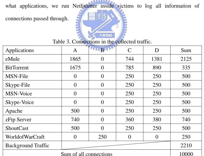
The traffic for evaluating our methodology is recorded from NCTU High Speed Network Lab and NCTU CSCC department. In the traffic recording environment, d, we select 4 "victim" PCs, say host A, B, C, D to run specified applications on them. The host "A" plays the role of server; it supplies the seed of P2P file sharing applications, and runs as Apache servers, zFTP servers and ShoutCast servers. Other interactive applications without our intervention are executed on host "B", like WorldfoWarCraft, MSN chatting, Skype chatting. The rests "C","D" play the role of receivers. For these victims, the purpose of tracing every connection that come from what applications, we run Netlimitter inside victims to log all information of connections passed through.
Table 3. Connections in the collected traffic.
Applications A B C D Sum eMule 1865 0 744 1381 2125 BitTorrent 1675 0 785 890 335 MSN-File 0 0 250 250 500 Skype-File 0 0 250 250 500 MSN-Voice 0 0 250 250 500 Skype-Voice 0 0 250 250 500 Apache 500 0 250 250 500 zFtp Server 740 0 360 380 740 ShoutCast 500 0 250 250 500 WorldofWarCraft 0 250 0 0 250 Background Traffic 2210
19
We collect traffic 50 samples total, and each complete one is defined by satisfying all the three following conditions: (1) the data from the seeds could be completely received by all peers; (2) a request from client is served by server side. For example, a download request from a client to the apache server is served; (3) Streaming services, such as a whole song has been played by ShoutCast server. As Table 3 shows that 77.9% connections are from the victims and 22.1% are from the background traffic of Speed Network Lab and CSCC department of NCTU..
4.2 Connection Recognition Rate (CR) and Accuracy
Figure 11: Connection Recognition rate
We compare the completeness of session association between our classification algorithms on the basis of the logs recorded from NetLimitter. The definition of one session for each application is defined as following (1) for P2P applications, one program executes continuously until stopping intentionally. (2) A client’s request is served completely by server. (3) A voice session runs without breaking off from beginning to end. The higher the connection recognition (CR) rate is, the more completeness of session association. The results are shown as Figure 11, and we can observe that, the recognition rate of applications use multi-connections are improved
0% 10% 20% 30% 40% 50% 60% 70% 80% 90% 100% Connection Recognition Rate CR with PAT
20
1.2 ~ 2 times. For those rates of evaluated applications are equal before and after using ports association algorithm (PAT) , there are two reasons. First, the applications use single connection like MSN-file transferring, MSN-voice chatting, Sky-file transferring, Skype-voice chatting and ShoutCast voice streaming. The second, the port number used is not continuous, like the command and data transferring of zFTP servers. We also can infer that the improvement via ports association algorithm depends on two factors, (1) how fast can we recognize a connection? (2) how accurate can we do it?
For the accuracy testing, an event “hit” occurred if a session is recognized correctly using our method. Therefore, we can define a metric, accuracy, the percentage of sessions recognized over all sessions recorded by NetLimitter. Figure 12 shows the accuracy for every application in our evaluation. It is significant that e p2p applications and well-known protocol applications such like Apache and zFTP server have very high accuracy, say 98% on average. But for Skype and MSN-voice chatting, it’s hard to be recognized by only PSDs due to they aren’t always similar.
The accuracy testing also reveals the quality of a center. If we choose a center by an un-popular implementation of the application, the accuracy may be worse due to the characteristics of less adoption..
4.3 Bitt rren 0% 4% A dist wro first caus conn Hit Rate False pos to nt eM ule A c % 0% 0 % 7% 0 As described ance betwe ong decision t one is if th ses the am nection is Accuracy 0% 10% 20% 30% 40% 50% 60% 70% 80% 90% 100% Hit Rate Figu itive rate a Table 4: Fa Apa che zF TP ser ver 0% 1% 0% 1% d in Section een vectors n of identif he two diffe mbiguous de too less to Bittorr ent eMul 100% 98%
Accur
ure 12: Acc and False n alse positive Msn-File Ms Voi 0% 9% 0% 17% n 3, the dec s and cente fying traffic erent applic ecisions; the o calculate e Skype‐ File Sk V % 96% 8racy for
21 curacy for se egative rat e/negative ra sn-ice Skype -File % 0% % 0% cision of cla ers. The rea c can be sep cation’s cen e second o enough inf kype‐ Voice Msn‐ File 80% 100%r Session
ession detec e ate of each e Skype-Voice 2% 18% assification ason that w parated into nters are too one is if the formation a Msn‐ Voice Apa e(H ) 74% 100n Recog
ction application Shout Cast W W 1% 3% is based on why our al o 2 kinds o o close in th e number o and to clas ach Http ) zFTP server 0% 100%gnition
. Worldof WarCraft U o 0% 4% n the Euclid lgorithm m f problems; he space, it of packets sify it into Shout Cast Wow 96% 96% Unkn own 7% 0% dean makes ; the may in a o the w %22
appropriate center that represent certain application. The first problem can be avoided by choosing appropriate centers that the distance between them is not too close. The other one can be done by collecting enough packets, and we will describe in next section in detail.
If a connection could not be divided into a given application correctly, it exhibits false positives. If it could not identify all connections of a given application correctly, it exhibits false negatives respectively.. Table 4 shows the false positive/negative rate in our traces. For zFTP server, the false positive occurs when we evaluate its’ command connection, and for streaming services, it happens when the PSD changes more violently than usual.
4.4 On-Line Gateway Architecture analysis
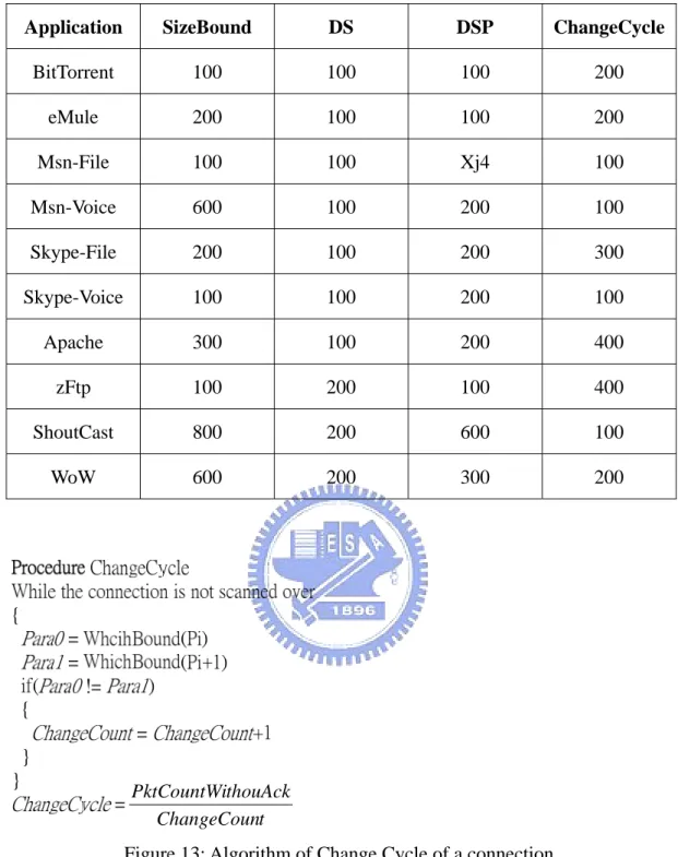
The key point of implementing our algorithm into on-line gateway architecture is on how many packets we should evaluate at least to obtain enough information to compute the connection vector. By the algorithm we mentioned above, we find that it will take at least one hundred of packets of a connection to obtain the stable connection vector. In our analysis, we calculate each entry of the connection vector in every 100 packets, and see if the value will converge to ± 5% to the representative values of the whole connection vector. Table 5 shows the convergent speed of each entry for each application. It takes one hundred to four hundred numbers of packets on average to obtain the stable entry values. For every application, we find that
SizeBound is the key factor because every metric we used needs to complete the SizeBound evaluation first.
23
Application SizeBound DS DSP ChangeCycle
BitTorrent 100 100 100 200 eMule 200 100 100 200 Msn-File 100 100 Xj4 100 Msn-Voice 600 100 200 100 Skype-File 200 100 200 300 Skype-Voice 100 100 200 100 Apache 300 100 200 400 zFtp 100 200 100 400 ShoutCast 800 200 600 100 WoW 600 200 300 200 t ChangeCoun thouAck PktCountWi
Figure 13: Algorithm of Change Cycle of a connection.
For on-line architecture, we propose a new definition of SizeBound in our algorithm and use it to count change cycle. We first divide one connection P into
four subsets of equal size, say Pd1 , Pd2 , Pd3 and Pd4 , where 4 ... 1 }, ,..., , { 1 2 ∀ = = P P P i
Pdi i i in . And define a “change” if packetPj∈Pdm, Pj+1∈Pdn,
24
number of packets that a change happened and using an algorithm as Figure 13 to describe. This approach provides faster decision but the accuracy will be decreased about 2% on average.
We then give a discussion for simple on-line device overhead evaluation. For storage overhead, every connection in the connection table needs 400 bytes (32bits*100) of memory storage, center database storage, and PAT cache storage. For processing overhead, the time of transforming a connection to a vector and access PAT cache will be the performance bottleneck .
25
Chapter 5. Conclusions and Future work
We observe two characteristics of transport layer behavior of applications from experiments. First, different implementations of applications produce different packet size distribution. The second is if an application use multi-connections sessions, then the port numbers used might be continuous. By utilizing these two features, it’s easy to distinguish different applications. As long as we can recognize one connection of the application by packet size distribution, we can use the characteristic of port locality to recognize other connections of the same application.
In this work, we design a classification algorithm that without accessing any packet payload information and obtain high accuracy at the expense of low false positive rate for applications which tend to transfer series data. Additionally, our method also works for encrypted applications, such as Skype file-sharing and voice chatting.
In the near future, we’ll evaluate other factors that may affect PSD, like Ethernet link type. It’s obvious that the size distribution of the same connection will be different in different network link type. For example, the MTU of Ethernet is 1500 bytes and PPP is 1492 bytes. We may need to evaluate different link types to decide which one is better to be the representative center of the application. Or we can separate connections of different link type into different spaces that contains centers which are pre-defined from different network link type.
Our methodology might be able to be combined with signature based classification method to get better effects. For example, signature based classification method works very well for Http applications. Therefore, our classification methodology can avoid calculating Http traffic but spend more effort on others. It means this method can be the second guard to classify those traffic that signature based method can’t recognize.
26
Reference
[1] S. Sen, O. Spatscheck, and D. Wang. Accurate, Scalable In-Network Identification of P2P Traffic Using Application Signatures. In Proc. World Wide Web Conference, 2004.
[2] Patrick Haffner, Subhabrata Sen, Oliver Spatscheck, Dongmei Wang. ACAS: Automated Construction of Application Signatures. SIGCOMM’05 Workshops, August 22–26, 2005,
[3] Angelo Spognardi, Alessandro Lucarelli, Roberto Di Pietro. A Methodology for P2P File-Sharing Traffic Detection, HOT-P2P'05 Second International Workshops
[4] V. Paxson. Empirically derived analytic models of wide-area TCP connections. IEEE/ACM Trans. Netw., 2(4):316–336, 1994.
[5] Manuel Crotti; Murizio Dusi; Francesco Gringoli; Luca Salgarelli; “Traffic Classification through Simple Statistical Fingerprinting”, 2007 ACM SIGCOMM Computer Communication Review on Volume 37, Number 1, January 2007
[6] Thomas Karagiannis, Andre Brodio, Nevil Brownlee, Michalis Faloutsos; “Is P2P dying or just hiding” Networking, IEEE/ACM Transactions on Volume 12, Issue 2, April 2004 PP.219 – 232.
[7] Thomas Karagiannis, Andre Broido, Michalis Faloutsos, Kc claffy, "Identification and classification: Transport layer identification of P2P traffic", October 2004 Proceedings of the 4th ACM SIGCOMM conference on Internet measurement.
[8] Thomas Karagiannis, Konstantina Papagiannaki, Michalis Faloutsos, "BLINC: multilevel traffic classification in the dark", Proceedings of the 2005 conference on Applications, technologies, architectures, and protocols for computer communications SIGCOMM '05.
[9] Netlimiter, http://www.netlimiter.com. [10] Wireshark, http://www.wireshark.org