繁衍形體

全文

(1)國立交通大學建築研究所碩士論文. Propagating Figures A Genetic Algorithm Approach. 繁衍形體基因演算法. 研究生指導教授. 王聰憲劉育東. 中華民國九十三年七月.

(2) Propagating Figures A Genetic Algorithm Approach. 繁衍形體基因演算法. 研究生指導教授. 王劉. 聰育. 國. 憲東. 立建. 交. Tsung-Hsien Wang. Advisor. Yu-Tung Liu. 通. 築碩. Student. 研. 大. 士. 究. 學. 論. 所文. A Thesis Submitted to Graduate Institute of Architecture College of Humanities and Social Sciences National Chiao Tung University in partial Fulfillment of the Requirements for the Degree of Master In Architecture. July 2004 Hsinchu, Taiwan, Republic of China. 中華民國九十三年七月.

(3) ABSTRACT A cognitive phenomenon, emergent subshapes, has been examined extensively in the last decade. From the cognitive perspective, “emergent subshapes” plays the important role in developing the design, and this phenomenon happens very frequently during the early conceptual phase. Based on this, various computational approaches also arise to explore this cognitive phenomenon, and the most well known of them are symbolic and connectionist approaches. To compare these two methods, one distinct discrepancy is that symbolism is good at efficient performance where connectionism excels in providing valid recognition. In other words, one focuses on providing abundant shapes and the other tries to recognize those useful, though few, subshapes. Therefore, the predominate problem statement of this study is how to propose a suitable mechanism to generate not only numerous but also valid subshapes. Moreover, after abundant explorations in design thinking, cognitive and computational approaches are already sufficient enough to provide computer-aided design (CAD) tool with a very substantial foundation. New computer media also bring designers a promising vision by means of its powerful computing capacity; notwithstanding, this is no more than prospect. Therefore, how to take advantage of the computational capacity to assist designers from a cognitive perspective is also the other significant issue in this study. Particularly, in order to make the computer media get closely involved into the process of designing rather than merely serve as a presenting tool, this study aims to propose a mechanism that could show the potential of not only recognizing subshapes but also allowing designers to interact with throughout the early conceptual phase. To specify this, how to achieve this objective will start from exploring the cognitive perspective—emergent subshapes, and then implement this mechanism as a CAD system to assist designers. Furthermore, in this study, genetic algorithm is adopted to tackle this issue. By means of the nature-like selection, the relationship of shapes and subshapes was reexamined; thus, from this point of view, genetic algorithm provides another approach—neither symbolism nor connectionism—to support designers in evolving more unanticipated subshapes. Ultimately, through integrating this mechanism into the three-dimensional modeling application, the combination of theoretical researches with computer-aided design could go further into a more practical and constructive stage.. Keywords: emergent subshapes, the early conceptual phase, genetic algorithm. iii.

(4) 摘要浮現子形這個現象在過去的十年間已經被大量的討論，特別是在設計初期的發展過程中，這個現象扮演著推進設計一個非常重要的角色。所以，在這個現象被提出之後，另外一群研究者從運算的角度來重新檢視這個現象，其中最知名的不外乎是形狀文法（Shape Grammar）、資料檢索模型 (Data-driven symbolic model)以及神經網路 (Connectionist networks) 等。這些方法最大的差異在於，前面兩種比較傳統的運算方式在對於產生很多形體的運算上很有效率，另外一個神經網路正相反，他提出了應該以尋找有效的隱含形體為主，而非是去尋找無限多的形。所以在本研究首要的目的便是希望可以提供一個方法，可以來同時處理多且有效的形的問題。此外，在大量相關的研究之後，這些認知與運算的研究已經提供了非常充足的基礎來建構一個電腦輔助設計系統，是以能夠從認知的角度為出發，透過電腦運算的能力來加強設計者的能力。這樣一來，電腦媒材才可以不僅僅是被當作呈現的工具，而進一步從運算的能力來輔助設計者。所以如何能夠從這樣一個研究的基礎為背景，進一步提出適當的電腦輔助設計工具 (computer-aided design tool) 是在本文另外一個重要的問題。所以，為了達到這樣的目標，在本研究中希望透過基因演算法，從一個演化的觀點來重新檢視這樣一個問題，最後，透過將這個方法整合到一個 3D 建模的環境，這樣一個結合理論研究與電腦輔助的工具將會更進一步推進到有效且實用的階段。. 關鍵字：浮現子形，設計初期階段，基因演算法。. -ii -.

(5) TABLE OF CONTENT. i. Abstract Abstract(Chinese) Chapter 1. Chapter 2. Chapter 3. Chapter 4. Chapter 5. References Appendix 1 Appendix 2. ii. Introduction 1.1 Scopes 1.2 Problem Statement and Objective 1.3 Methodology and Steps Emerging Shapes 2.1 Cognitive Emergent Subshapes 2.2 Computational Emergent Shapes 2.3 Genetic Algorithm and Knowledge Representation Data Structure and Genetic Framework 3.1 Data Structure Two Kinds Of vertices Operational Chromosome 3.2 Genetic Framework The Fitness Measure Selection Methods Genetic Operations Set Population Size Termination Criteria System Construction and Specification 4.1 System Overview 4.2 System Specifications 4.3 Fitness Validity 4.4 Demonstration Conclusion 5.1 Analyses and Comparisons 5.2 Significance 5.3 Limitations and Future Studies. [ 01 ] [ 02 ] [ 04 ]. [ 06 ] [ 09 ] [ 11 ]. [ 14 ] [ 14 ] [ 15 ] [ 16 ] [ 16 ] [ 18 ] [ 19 ] [ 21 ] [ 21 ]. [ 23 ] [ 28 ] [ 32 ] [ 35 ]. [ 40 ] [ 42 ] [ 43 ] [ 44 ]. Activations of Single-Gene Chromosomes System Codes. ii. [ 46 ] [ 48 ].

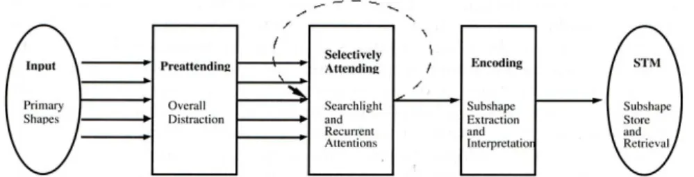
(6) CHAPTER 1 INTRODUCTION. CHAPTER 1. INTRODUCTION. 1.1 Scopes Design process, in a sense, is a kind of search based on visual processing (Schon and Wiggins, 1992; Liu, 1996b; Oxman, 2002). Within this visual search, shapes play the most indispensable role and in general, these shapes, in light of different contexts and conditions, could present different meanings and contents (Gero and Yan, 1993; Soufi and Edmonds, 1996). That is to say, even those incomplete figures, ambiguous and uncertain, could provide designers with plentiful information, especially during the early conceptual phase. Thus, designers could integrate the information they received with the images emerged, and further make design progress. During the design process, visual interactions articulate what designers move according to what they perceived and considered inside their minds (Schon and Wiggins, 1992). Within this, one cognitive phenomenon—emergent subshapes—was proposed. Most importantly, designers have their distinct gaps in recognizing subshapes, and at the same time, the greater part of shapes must be searched for instead of emerging effortlessly (Liu, 1995). Moreover, the more complex the shapes are, the more time designers need to find them. Besides, these emergent subshapes, in general, do not exist explicitly in the original shapes but do have the indispensable relationship with the original ones and the significant influence on the following design. From the cognitive and computational model of restructuring shapes proposed by Liu (1996a), it signifies two major steps in restructuring emergent subshapes. One is selecting (from pre-attending to selectively attending) and the other is encoding (Figure 1.1). Similarly, Soufi and Edmonds (1996) also regarded these emergent subshapes as the results not only from perceiving the external stimuli but also from transforming the internal structures. To summarize, these emergent subshapes appear when 1) designers perceive/select certain shapes, and 2) further restructure these shapes into new configurations of them.. Figure 1.1. A cognitive and computational model of restructuring shapes in terms of emergent subshapes (after Liu, 1996a). In addition to cognitive examinations, computational approaches also arise to PROPAGATING FIGURES. -1-.

(7) CHAPTER 1 INTRODUCTION. investigate this phenomenon, emergent subshapes. Such as shape grammar, it provides a productive way to recognize or, say, generate emergent subshapes by means of symbolic notations and rule-applications (Stiny, 1978, 1980, 1993; Knight 2003a, b). Or, Gero and Yan (1993) proposed a data-driven symbolic model to discover emergent subshapes from infinite maximal lines and generated so-called phantom shapes eventually. More, Liu (1993) submitted a connectionist system trained to recognize emergent subshapes from the opposite way. All these computational methods addressed their own fashions of how computers recognize those emergent subshapes that human designers could under certain conditions. Ultimately, on the strength of rapid development in artificial intelligence, there is one another prevailing mechanism, genetic algorithm, available to tackle those particularly intangible problems. More specifically, based on nature selection, the fundamental principles of genetic algorithm (GA) were first proposed by Holland (1975). Through genetic evolutions and competitions, a chromosome, which has the better fitness, is more likely to survive and thus becomes the potential solution under current condition. Moreover, by employing such a population-based search, GA has been used in a variety of disciplines, including art, music, or architecture (Bentley, 1999; 2002). In this regard, this mechanism reveals a great capability of solving those complicated and intangible problems, which are exactly the same as the problems in design, from utilizing this biologically inspired approach (Mitchell, 1996).. 1.2 Problem Statement and Objective Under most circumstances in design, drawings always play the most important role in externalizing designers’ ideas. Moreover, through interacting with these drawings, designers make their design proceed. Within this process, emergent subshapes are the key media responding to what designers consider in their minds and this happens very frequently especially when designers try to reexamine what they have drawn under distinct conditions. Based on this point of view, Minsky (1986, p.144) proposed that “the way we perceive the world, from one moment to another, depends only in part on what comes from our eyes: the rest of what we see from inside our brain.” As a result of Minsky’s statement, it implies that there should be two steps of recognizing shapes. One is what we perceive from the external stimuli and the other is what we restructure inside our brains, such as rules applications or knowledge transformation, etc. That is to say, first of all, designers look at the given shapes, so-called the external stimuli, and then PROPAGATING FIGURES. -2-.

(8) CHAPTER 1 INTRODUCTION. restructures what they have seen and what they are contemplating in their minds, so-called the internal transformation. Therefore, the first step could be just served as to see (perceiving) and the second is to restructure (transforming). In this case, a suitable mechanism that is intended to tackle the problems deriving from emergent subshapes should be beneficial in both these two steps—perceiving and transforming. However, notwithstanding symbolic and connectionist approaches have been employed on this issue tremendously, it is still hard to satisfy designers in recognizing subshapes with fixed rules and limited recognition. To specify this, on the one hand, symbolism submits an efficient computational way in generating numerous shapes by means of notations and rule-applications. On the other hand, connectionism attempts to recognize shapes in terms of connecting vast artificial neurons from an opposite respect. Both of them, without doubt, address some advantages in generating or, say, recognizing shapes. Yet, it seems still insufficient in recognizing emergent subshapes from neither symbolic nor connectionist approaches. Such as, symbolic processing usually generates emergent subshapes only when there are already the rules specified. Therefore, although this mechanism could generate numerous subshapes, those generated subshapes are relatively limited to certain anticipated scopes. In other words, only when the left hand side of rules is matched, the corresponding shapes are generated. Obviously, this is deficient in perceiving part of recognizing subshapes. In addition, connectionist processing proves its success in recognizing subshapes especially from ill-structured or incomplete shapes. In this regard, this useful recognition can provide designers more feasible recognition and simulates how designers recognize shapes. However, the vulnerable point of connectionism is always the limited training patterns; sometimes, with respect to the limitations of the small quantity of trained patterns, it reminds us of performance inefficiency. In other words, although connectionism has a great adaptation in recognizing those ill-structured shapes, its limited training patterns confines its capability in restructuring these perceived shapes. Therefore, how to propose a robust mechanism that could show a power capability in both perceiving and transforming steps of recognizing subshapes becomes the major problem statement in this study. In addition, whereas emergent shapes play such an important role in design process and meanwhile have the great relevance to creativity, another significant issue proposed in this study is how to provide a computer-aided design (CAD) system to support designers in search for more promising subshapes. Therefore, by means of amplifying the amounts of emergent shapes, designers could be inspired and further evolve the innovative designs. Therefore, in order to propose a suitable mechanism to tackle the problem of recognizing emergent subshapes, genetic algorithm is here proposed. From genetic PROPAGATING FIGURES. -3-.

(9) CHAPTER 1 INTRODUCTION. perspective, no matter how gene is selected and further evolved, it is manifest that a crucial relationship of inheritance and similarity does exist between parents and offspring. Moreover, the relationship between parents and offspring is analogous to the relationship of shapes and subshapes or the sum of shapes and subshapes in this study. Particularly, those intangible and ambiguous problems have been proved and solved successfully by means of genetic algorithm (Man, Tang and Kwong, 1999). In this regard, genetic algorithm (GA) signifies the prospect of dealing with the issues with respect to emergent shapes, those exactly having the identical characteristics of ambiguity and uncertainty in design. To summarize: 1) Neither symbolism nor connectionism is sufficient enough to tackle the problem of recognizing emergent subshapes. 2) Emergent subshapes play such an essential role in making design progress. 3) Moreover, these emergent shapes usually have a profound influence on the following design, and have a significant relevance to creativity. The major objective of this study expects to propose a suitable mechanism to reexamine the cognitive phenomenon, emergent subshapes, from an evolutionary perspective. Moreover, by means of implementing this mechanism into a physical system, this study further expects this evolutionary system can provide designers more accesses to evolve designs, especially during the early conceptual phase. In this regard, it will be used to help designers in generating more shapes and providing more stimulation. Ultimately, in terms of the expansion of the emergent behaviors, designers could evolve innovative designs from a biological evolutionary perspective.. 1.3 Methodology and Steps In order to achieve the objective of providing a suitable mechanism of recognizing and reconfiguring shapes, there are several principal procedures. However, in order to specify this process more efficiently, I take two-dimensional shapes as a foundation to explore basic evolutionary mechanism. Therefore, the first section with respect to basic data structure and genetic framework is articulated through two overlapping rectangles as the preliminary research. Then, by means of implementing this mechanism into the three dimensional modeling environment, a computer-aided design system is hence conducted. Eventually, through a demonstration, more complex and more efficient performance is crystallized. For more details, all these procedures are discussed as follows: PROPAGATING FIGURES. -4-.

(10) CHAPTER 1 INTRODUCTION. 1). 2). 3). Data structure: Two kinds of vertices are examined to construct the fundamental data. One of them is termed as the embedded vertex (EV), which is encoded by the original coordinate values of the current shapes. The other is the invisible vertex (IV) conducted from the intersections of extending polylines. Afterwards, the basic operational units are produced according to these basic vertex data (EV and IV), and these smallest units, in more detail, are the most essential components for the next stage. Genetic algorithm framework: In order to provide a CAD environment without firing rules, the generative mechanism is contrived mainly from genetic algorithm to simulate the process of nature selection. Through several steps, including initialization, evaluation, propagating (such as selecting, crossover, mutation and reproduction) and terminating, this mechanism could be used to handle the problem of recognizing subshapes during the design process. System construction and specification: After articulating the genetic algorithm, an evolutionary system is constructed and relevant system components are specified. During this section, first of all, the overview of this system is described. Secondly, system components are proposed. Third, single-chromosome gene is examined to see the validity of fitness. Finally, a physical manipulating process is demonstrated.. In sum, on the strength of combining the genetic algorithm with shape emergence, this generative system aims to assist designers during the early conceptual phase to propagate more promising emergent shapes. Moreover, considering some inseparable connections to creativity, such a tool signifies the potential to improve the creativity in terms of amplifying the quantity of the emergent shapes. However, to build a more intelligent system, it should allow designers to interact with this system more easily. Therefore, in this study, by integrating into the current popular application, Alias|Wavefront MAYA—a three-dimensional modeling software, this mechanism, implemented by Maya Embedded Language (MEL), provides designers with more eligibility during the design process. Ultimately, this study could contribute profits in both cognitive and computational domains.. PROPAGATING FIGURES. -5-.

(11) CHAPTER 2 EMERGING SHAPES. CHAPTER 2. EMERGING SHAPES. An emergent shape is a shape that exists only implicitly in a primary shape, and this shape is never explicit input and is not represented at input time (Mitchell, 1992b).. As a well-know behavior, designing proceeds through a sequence of seeing-moving-seeing circulation (Schon and Wiggins, 1992). Based upon what he perceived, a designer conducts his next moves. Moreover, during this period, the visual representation-and-interaction behavior plays the most significant role in communicating designers and design-representing tools. Simultaneously, the cognitive phenomenon of emergent subshapes, which happens very frequently when a designer attempts to make his next move, has also proved the capability in making design proceed during the early conceptual phase. Therefore, two essential domains, including cognitive and computational researches relevant to shape emergence, arise in this research. In addition, in order to tackle the issue deriving from shape emergence, genetic algorithm is served as the major mechanism in this study. All these relevant researches will be introduced in this Chapter. In the beginning, the first section will start from discussing cognitive researches with respect to emergent subshapes. For example, when these subshapes appear, how these subshapes could be recognized or the significant characteristics of emergent subshapes—all these will be described to form a cognitive framework of emergent subshapes. Subsequently, the second section addresses several computational approaches, which are mainly used to generate or recognize these subshapes concealing under the primary shapes. Such as, shape grammar, data-driven symbolic model, connectionist network and so on—these approaches all take distinct computational perspectives to investigate the cognitive phenomenon, emergent subshapes, from a generative perspective. Finally, genetic algorithm (GA) is discussed briefly and Knowledge representation of chromosome is introduced.. 2.1 Cognitive Emergent subshapes 2.1.1 Shape Emergence Since emergent subshapes are proposed, during this iterative and ceaseless process—seeing, moving and seeing, this visual phenomenon elucidates when and how PROPAGATING FIGURES. -6-.

(12) CHAPTER 2 EMERGING SHAPES. subshapes are extracted from parts or the sum of parts of shapes, and therefore play an important role in directing the further explorations in design process (Gross, 1995; Soufi, 1996; Oxman, 2002). Moreover, how a designer discerns the sub-shapes from a cognitive perspective and what a designer proceeds through visual perceptions were proposed to examine the relationship between designers and drawings (Soufi, 1996). For example, emergent shapes, by means of the diverse decompositions of shapes in any phase of the design process, could be generated infinitely under distinct contexts. In others words, emergence could be extracted from whether the sum of shapes or the part of shapes and there is no absolute standards for extracting subshapes from primary shapes (Holland, 1999; Stiny, 2001). 2.1.2 Tow Steps in Recognizing Emergent Subshapes In the other perspective, pertinent to the perception of shapes emergence, designers often recognize subshapes from certain contexts, attentions, purposes and interests (Testa, 2001). Based on different conditions, designers could detect different subshapes and drive their design into different directions. Similarly, Oxman (2002) also submitted that the manipulations of visual schemas and prototypes enable to generate more alternatives. Thus, some researches further presented, within this process, there should be certain attention and guidance before perceiving or, more correctly, searching for emerging shapes (Liu 1995; Oxman 2002). For example, designers might pay pre-attention into certain area first, where they interest under current context, and then further reconsider the subject again and again and therefore conduct their next steps. That is to say, when we look into the more details of shape emergence, how to recognize subshapes could be synthesized as two major steps. One is to perceive the intended subject from part of original shapes. The other is to restructure these selected shapes by means of relevant domain knowledge (Liu, 1996a). Regardless of how to perceive these selected shapes in advance, designers interpret the shapes in their own fashions and then restructure the shapes (Soufi, 1996). To summarize, a complete process of shape emergence has a dual-process in the search of subshapes—perceiving and restructuring (Figure 2.1).. Figure 2.1. PROPAGATING FIGURES. Two Steps in recognizing emergent shubshapes.. -7-.

(13) CHAPTER 2 EMERGING SHAPES. Although how to recognize those sub-shapes from the existing shapes seems as only one of the most trivial human behaviors, it’s better to regard this behavior, recognizing emergent subshapes, as to ‘search for’ them rather than ‘seeing’ them effortlessly (Oxman, 2001). Particularly, some of these subshapes might be more difficult and laborious to detect, such as those unnamable ones (Liu, 1995). Thus, in a sense, emergent shapes are predictable in the process of generation; nevertheless, when an emergent shape could be discerned is still unpredictable (Stiny, 2001; Knight, 2003). 2.1.3 The Classification and Corresponding Activations of Shapes After the considerable accumulation of useful investigations, some researchers set out to categorize these emergent shapes. Liu (1995) submitted that shapes could be classified into explicit、implicit、closed and unclosed shapes which are first mentioned by Mitchell (1992), and proposed four significant phenomena in recognizing these subshapes. Within this, the time designers need to recognize a subshape is in proportion to the complexity and visibility of the subshape. Figure 2.2 represents these four different compositions of subshapes.. a.. closed and explicit. b.. unclosed but explicit. c.. closed but implicit. d.. unclosed and implicit Figure 2.2. Four kinds of shapes (after Liu, 1998).. Besides, there is still one more specific element proposed, which is termed as “the threshold of recognizing activation (TRA) value” (Liu, 1995). This value is particularly used to discern the discrepancies between expert and novice designers in recognizing these emergent subshapes. In Liu’s research, when this TRA value is integrated into connectionist networks, different subshapes with different activations could be recognized in turn. For example, when the TRA value is 0.98, only Figure 2.3a. could be extracted. Following this, when this TRA value is decreased to certain degree, say, 0.8, three more other figures—Figure 2.3b., Figure 2.3c., Figure 2.3d.—could be extracted. Within this process, one interesting finding is that those subshapes, existing implicitly and unclosedly at the beginning, are the hardest ones to be extracted and in general, only those expert designers who have lower TRA value could recognize these subshapes. This implies some order but also limitations in extracting these subshapes; therefore, from this way, subshapes could be recognized more systematically.. PROPAGATING FIGURES. -8-.

(14) CHAPTER 2 EMERGING SHAPES. Figure 2.3. TRA values versus subshapes encoded by connectionist networks (refined after Liu,1995).. In addition, in the process of shape emergence, shapes are distinguished as anticipated, possible or unanticipated ones (Knight, 2003b). From Knight’s definitions, unanticipated shapes could show the capability of handling rules extragrammatically. Moreover, in general, the appearance of emergence always accompanies with ambiguity. As is stated above, that, ambiguity, is exactly one of the most important characteristics of emergent subshapes, and by means of this characteristic, any implicit subshapes are possible. More, when Soufi (1996) classified the shapes from the composition of shapes, such as those boundaries of subshapes, subshapes could be just regarded the same as those of the original shapes or part of them. Or, shapes could also arise as a result of occlusion, including the combinations of the extending boundary lines, existing points or new points resulted from the intersections of the extending boundaries, etc. Oxman (2002) proposed a binary perspective which comprises perceptual and cognitive components to specify the emergence in design process. In brief, with ample explorations in visual thinking, this phenomenon, which we termed it as shape emergence, was proposed and pertained to the characteristics of uncertainty and ambiguity (Mitchell, 1992; Soufi, 1996; Suwa, 1999; Stiny, 2001; Testa, 2001). In terms of these characteristics, subshapes could be extracted from the primary shapes, no matter existing explicitly or implicitly at the beginning. However, though, these characteristics are sometimes a prospect, but also a hindrance at the same time, to an opportunity of extracting unexpected subshapes.. 2.2 Computational Emergent Shapes 2.2.1 Shape Grammar Sequentially, from computational point of view, there are diverse approaches in generating shapes; some of them are applied to investigating emergent subshapes. For example, shape grammar was first proposed by Stiny and Mitchell (1978). In that research, shape grammar was used to generate certain villa-style planes, which is used to simulate what Palladio might do. In this case, shape grammar could be simplified as a mechanism to generate Palladian-style planes by means of symbolic notations and PROPAGATING FIGURES. -9-.

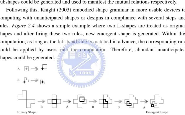
(15) CHAPTER 2 EMERGING SHAPES. rule-applications derived from original Palladio’s design disciplines. For a more implementation purport, Nagakura (1990) tried to use a script-based approach to recognize, and transformed shapes on the basis of shape grammar. Starting from categorizing abundant shapes, which is mainly defined as a set of successive lines, this approach used pre-coded scripts of the drawing “D” and categorical objects “O” and categorical transformations “T” to “Find” possible subshapes (where “Find” is the control command in this research). Eventually, stylistic geometry could be generated through a pattern-matching process. Besides, in 1993, Stiny further used this mechanism in generating subshapes. He used rules in reinterpreting the relationships of the way what designers perceive, and how they move after perceiving. By means of ambiguity of descriptions, possible subshapes could be generated and used to manifest the mutual relations respectively. Following this, Knight (2003) embodied shape grammar in more usable devices to computing with unanticipated shapes or designs in compliance with several steps and rules. Figure 2.4 shows a simple example where two L-shapes are treated as original shapes and after firing these two rules, new emergent shape is generated. Within this computation, as long as the left-hand side is matched in advance, the corresponding rule could be applied by users into the computation. Therefore, abundant unanticipated shapes could be generated.. Figure 2.4 This is a grammar example after Knight(2003b). Within this figure, two rules and original shapes are presented. Through five steps, new combination of shapes could be generated.. 2.2.2 Data-Driven Symbolic Model In addition to these finite shapes, Gero (1993) proposed another data-driven symbolic model to explore emergent subshapes. In this study, there are two dominant steps—one is termed as constraint derivation and the other is termed as shape discovery. As shown in Figure 2.5, this mechanism first unstructured the original input shapes into hiding shapes; then, by means of deriving new constrains that do not exist at the first input time, a data-driven search method was used to construct suitable polyline shapes—emergent shapes. Within this study, the most interesting thing is that those so-called “phantom shapes” could also be discovered. PROPAGATING FIGURES. - 10 -.

(16) CHAPTER 2 EMERGING SHAPES. Figure 2.5. In terms of infinite maximum lines, emergent subshapes could be generated, especially those “phantom shapes” that could not be generated by shape grammar (redrawing after Gero and Yan, 1993).. 2.2.3 Connectionist Networks Except for symbolic approaches, Liu (1996b) further suggested a connectionist networks trained to recognize these emergent subshapes, including explicit, implicit, closed or unclosed ones. Within this connectionist networks, searchlight attention, current attention and extracting mechanisms are used to reinforce the recognizing ability of it. Finally, in addition to emerging subshapes, this study also clarified one cognitive phenomenon in regard to designers’ visual behaviors—the threshold of recognizing activation. By means of this, connectionist networks could successfully simulate how a human designer recognizes these emergent shapes. Therefore, a computer system proves the ability to generate those useful subshapes rather than merely providing enormous alternatives. In brief, all these researches provide an integral foundation to inspect this significant phenomenon of shape emergence in visual thinking, not only from cognitive but also from computational point of views. Moreover, the more important thing is that shape emergence has an inseparable relationship with creativity as well and still not to clear up yet (Soufi, 1996;Ueda, 2001; Oxman, 2002; Knight, 2003). Whereas it does imply one exciting prospect in developing novel designs in terms of expanding this behavior of emergence during the design process, there should be more efforts in exploring more and useful emergent shapes from both cognitive and computational way.. 2.3 Genetic Algorithm and Knowledge Representation 2.3.1 Genetic Algorithm With the rapid development in artificial intelligence, more and more intelligent exploitations in the design researches arise to simulate how a human designer could do (Bentley, 2002). Such as so-called evolutionary computation, it submits a feasible way to solve the complex problems based on nature selection and evolutionary searches. Among these mechanisms, genetic algorithm (GA), originally proposed by Holland, J.H., has been substantially applied into diverse disciplines. It was primitively inspired. PROPAGATING FIGURES. - 11 -.

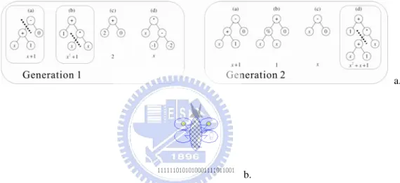
(17) CHAPTER 2 EMERGING SHAPES. from the Darwinian principle of nature selection. Through closely mutual competitions, those individuals who have better fitness would have a great probability to survive. Moreover, in general, GA is one kind of the population-based search. Once new “building block” appears, new offspring will converge toward this tendency. The only way to get out of this convergence is use mutation operator. By introducing variations into the current populations, GA could rediscover new populations. Therefore, another good “building block” of solutions that are conferred higher fitness will eventually evolve. Besides, from another respect inside genetic operations, no matter how gene is selected and further operated, it is manifest that between parents and offspring exist one crucial relationship of inheritance and similarity (Figure 2.6). That is the reason why these populations look “similar”. Thus, this very relationship would be further analogized to examine the relationship between shapes and subshapes afterwards. In more details, the entire evolutionary process consists of the gene structure of a chromosome, several genetic operators, control function sets, the fitness measure, the terminal criterion, etc. During such a evolutionary process, a near-optimal solution could be possibly generated and presented by means of the fitness survival. Particularly, those intangible and ambiguous problems have been proved and solved successfully and efficiently by using genetic algorithm (Man, Tang and Kwong, 1999). It signifies the prospect of dealing with the issues concerning shapes, those exactly having the characteristics of ambiguity and uncertainty in design.. Genotype Figure 2.6. Phenotype. No matter how populations evolve, there must exist certain degree of similarity and inheritance reciprocally (after Bentley, 2002 ).. 2.3.2 Knowledge Representation of Genetic Algorithm Before starting the evolutionary process, one of the fundamental steps is chromosome representation. In terms of different problem conditions, there are various ways in representing chromosomes. For example, the conventional GA is developed on the basis of the scheme theory (Figure 2.7). Within this simple GA operation from Koza (1992), two fundamental ingredients are specified. One is the function set, and the other is the terminal set (2.1). T = {X, ℜ};. PROPAGATING FIGURES. F = {+, -, *, %}. (2.1). - 12 -.

(18) CHAPTER 2 EMERGING SHAPES. Where ℜ denotes constant numerical terminals in some reasonable range [ –5.0 , +5.0], and when whose output value is equal to the values of the quadratic polynomial x2+x+1 in the range from –1 to +1, this system terminate.. Sequentially, by means of recombination of two selected populations of the “Generation 1”, the desire solution is propagated in the “Generation 2”. All these manipulations could be presented in graph expressions. In addition, the bit string representation, in general, is also the other useful coding method and is adopted extensively. As shown in Figure 2.7, an insect is presented in a 25-bit long binary string. Different bits of this string are used to present different portions of the body, including color, size, texture, etc. Typically, based on bits flipping between the statuses of 1 or 0, the useful information could be restored and be retrieved in the future.. a.. b. Figure 2.7. a. graph expressions (After John Koza, 1992); b. binary string representation (after Man, Tang and Kwong, 1999). PROPAGATING FIGURES. - 13 -.

(19) CHAPTER 3 DATA STRUCTURE AND GENETIC FRAMEWORK. CHAPTER 3. DATA STRUCTURE AND GENETIC FRAMEWORK. In this research, emergent subshapes are regarded as one of the most important role during the early conceptual phase. Moreover, how to encode these schematic data into certain codes that machine could recognize is the primary step before further proposing a feasible system. During this early conceptual phase, designers usually draw scratchy diagrams to record or externalize their immediate concepts and ideas. At the same time, these diagrams, in general, encompass various and plentiful information with respect to any possible proposals. Designers, under this circumstance, reexamine what they have drawn iteratively, and therefore generate new combinations of part of old or new diagrams. Thus, in order to achieve the objective of providing a suitable mechanism in restructuring shapes by means of genetic algorithm, there are several principal procedures. However, as a preliminary step in constructing the basic mechanism, this research takes rectangle shapes as the dominate subjects. Moreover, only rectangles are discussed in this research. Eventually, through this 2D diagram, including two overlapping rectangles, the exhaustive search is constructed to reexamine the relationship among these small emergent units reciprocally. In more details, this first section includes: 1) the data structure of input and output, and 2) the structure of chromosome. Following this, the second part of this chapter describes the genetic framework in this study. By means of defining genetic operations, including crossover, mutation, production and evaluation, new populations, subshapes, could be evolved. All these fundamental genetic operations are refined from Man, Tang and Kwong (1999). After this, the preliminary step of this study is complete.. 3.1 Data Structure In this step, two major sub-procedures are articulated. One of them is the data structure of this program, and the other is to submit the most basic operational units, genes, of this system. 3.1.1 Two Kinds of Vertices First of all, all the input figures would be transferred into vertex data. For example, a line consists of two vertices and similarly, an enclosed plotlines-shape is viewed as one PROPAGATING FIGURES. - 14 -.

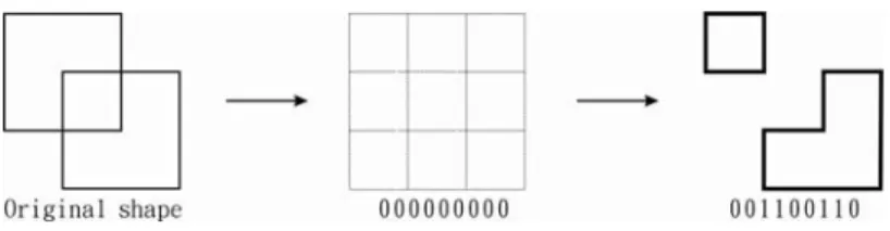
(20) CHAPTER 3 DATA STRUCTURE AND GENETIC FRAMEWORK. circuit of four vertices. Therefore, after designers draw some figures in working environment, this system would first interpret these figures into the primitive vertex data consisting of two dimensional coordinate values (Figure 3.1a.). As stated above, in order to demonstrate the whole process concisely, this study takes two-dimensional rectangle figures as the example in this section. The way applied in three-dimensional environment in the following section is identical. Figure 3.1 shows how to encode these two square shapes into vertex data. During this step, two kinds of vertices are generated. One is termed as the embedded vertex (EV) and the other is the invisible vertex (IV). EVs are those vertices embedded inside the original shapes or, say, the end points of original boundary lines (Figure 3.1a.). These vertices, in general, are visible and explicit at the input time. On the contrary, IVs are the vertices implicit at the input time and these vertices, in general, are generated from the intersections of extending lines and original boundary lines, as shown in Figure 3.1b.. a.. b.. Figure 3.1 (a) Embedded Vertices (End points); (b) Invisible Vertices (intersections).. 3.1.2 Operational Chromosome. After transferring the input figures into coordinate vertex data, there is still an indispensable step needed to be conducted in advance of having these data into the reasoning machine. A basic operational unit structure, chromosome, is therefore proposed and generated according to these vertex data. As stated above, the basic formation of this chromosome adopted in this study is rectangular. Therefore, by means of confining the category of emergent shapes, an exhaustive relationship could be reexamined in this research. Therefore, a gene could be regarded as a rectangle, which consists of either vertices embedded or invisible vertices or both of them. Most importantly, these small rectangle units, genes, should never be intersected by any other extending boundary lines (Figure 3.2a). In this regard, the new sub-boundary is emerged and the basic operational gene structure is generated. Sequentially, the relevant information of these genes would be preserved in a set of parameters structured by a string of value in binary form. As shown in Figure 3.2, a primary shape of two overlapping rectangles would be encoded as a 9-rectangle chromosome. Therefore, every bit of this 9-bit long binary string exactly represents every gene of this chromosome. Moreover, based on bits flipping between the statuses of 1 PROPAGATING FIGURES. - 15 -.

(21) CHAPTER 3 DATA STRUCTURE AND GENETIC FRAMEWORK. or 0, the visibility of the corresponding gene is altered. In this study, the bit value of “1”. represents a visible gene. On the contrary, the bit value of “0” represents the invisible one. Thus, by means of replication or recombination of these binary strings—parents, new offspring could be propagated.. Figure 3.2 a: Operational units (genes of chromosome); b: Binary string representation.. 3.2 Genetic Framework As stated above, the major objective of this study expects to take advantage of genetic algorithm to provide more feasible and promising shapes or subshapes for designers during the early conceptual phase. According to the evolutionary characteristics, including crossover, mutation, selection, fitness function, terminal criteria, etc., all these genetic operations outline the fundamental genetic framework in this study. All methods are described below. 3.2.1 The Fitness Measure During a genetic operation, the fitness function is always necessary and used to evaluate the status of a chromosome to see how “good” it is. Without a doubt, all the offspring propagated have to go through this evaluating process; therefore, those fitter ones could hence be preserved and others could be eliminated. Moreover, in general, this very fitness function set plays the predominant role with respect to the objective space specified by users. Before starting, I would like to review the threshold of reorganization activation (TRA) briefly in advance. This value, a specific parameter of evaluating the threshold of designers in recognizing subshapes, has been proved to tell apart the discrepancy between expert and novice designers from the cognitive point of view (Liu, 1996a). Therefore, by echoing this TRA value, this study initiates with ranking distinct weights according to the degree of the completeness of figures individually, and based on this, further expects to simulate how designers recognize subshapes from the computational perspective. Within this ranking process, the more complete the shape is, the higher weight it will score. Figure 3.3 denotes how distinct weights rank according to the. PROPAGATING FIGURES. - 16 -.

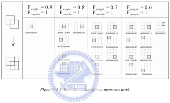
(22) CHAPTER 3 DATA STRUCTURE AND GENETIC FRAMEWORK. degree of completeness of shapes. In this case, three kinds of line segments are specified: 1) The explicit line segment: this represents explicit lines derived from cleaving original boundary lines by EVs and IVs, and has the index value of “1”; 2) The implicit line segments inside the original boundary: this segment includes every possible extending line segment, which does not exist at the input time, and locates inside the original boundary. The index value of it is “0.5”; 3) The implicit line segments outside the original boundary: different from the formers, the third line segments represent those other extending line segments, existing implicitly outside the original boundary, and have the index value “0.25”. Therefore, as shown in Figure 3.3, Fu5 comprises four explicit line segments and get the total index value “12”. In this case, the Fweight of overlapping area (Fu5) is designated to “1”, which is calculated from the ratio of the index value to the maximal value one operational unit could score. Following this, the rest may be deduced by analogy: 1) Fweight of U2, U4, U6 or U8 respectively is equal to “0.875”, including three explicit line segments and one implicit line segment inside the original boundary; 2) Fweight of U3 or U7 respectively is equal to 0.75, including two explicit line segments and two implicit line segments inside the original boundary; 3) Fweight of U1 or U9, respectively is equal to 0.625, including two explicit line segments and two implicit line segments outside the original boundary. To summarize, in Figure 3.3, the value of FU5 is greater than that of FU2 (which is equal to FU4, FU6 and FU8); FU8 is greater than FU3 (which is equal to FU7); FU7 is greater than FU1 (which is equal to FU9). Thus, after ranking all these units, several phenomena appear: 1) The fittest gene is generated from the overlapping area of two original shapes, and its boundary lines are exactly parts of the boundary lines of original shapes. 2) The adjacent relationship between other genes and the overlapping one decides the degree of Fweight. In general, the more the gene is close to the overlapping one, the fitter value this gene would score. 3) Moreover, genes inside the original boundaries always have higher fitness than those others outside the original boundaries.. Figure 3.3 Weights Ranking.. PROPAGATING FIGURES. - 17 -.

(23) CHAPTER 3 DATA STRUCTURE AND GENETIC FRAMEWORK. In addition, there is still one another fitness measure taking account of the complex-degree of units (Fcomplex). To specify this, the more the Fcomplex is, the more complex the chromosome would appear. Every different value of Fcomplex represents the distinct maximum number of genes that could turn to visible. Figure 3.4 shows how these two fitness measures work. For example, when {Fweight = 0.9 & Fcomplex =1}, only overlapping area, gene5, would appear; when the value of Fweight is decreased from 0.9 to 0.8, other four different chromosomes would be appear in turn. Eventually, this population-based search could proceed and generate fitter offspring with respect to the objective status, Fweight and Fcomplex. By altering the parameters of two fitness measures, qualified offspring could therefore survive.. Figure 3.4 A demo shows how fitness measures work.. 3.2.2 The Selecting Method In this section, in order to make sure new offspring could have a better fitness, this system provides one selecting method to decide the proportion of every parent in reproduction. Therefore, this step could be used to prevent premature convergence. In this study, Roulette Wheel selection is adopted, which is one of the most common methods for a proportionate selection (Man, Tang and Kwon, 1999). To specify this, the first step is to calculate the sum of all the parents in the mating pool (Fsum). By means of randomly selecting a number “n” between 0 and the Fsum [0 <n< Fsum], One parent would be selected, and in this case, the fitter the chromosome is, the possibility to be selected is higher. As shown in Figure 3.5, this Roulette wheel has the circumference from summing the five chromosomes. Chromosome 4 is the fittest one and hence has the largest interval. Therefore, a random number from the interval [0, Fsum] has the highest chance to select chromosome 4 in reproduction.. PROPAGATING FIGURES. - 18 -.

(24) CHAPTER 3 DATA STRUCTURE AND GENETIC FRAMEWORK. Figure 3.5 Roulette wheel selection (after Man, Tang and Kwon, 1999 ).. 3.2.3 Genetic Operation Set During the genetic algorithm operations, the most important mechanism is the re-combining process of the gene structures of parents. Therefore, in this section, all genetic operators available in this research, including four crossover methods and one mutation and one reproduction, are addressed as follows: 1. One-point crossover: This method is mainly used to recombine the given parents to generate new chromosomes by means of one crossover point. Figure 3.6 indicates how to perform this procedure. In details, one crossover point with the interval [1, 9] could be randomly selected and then the new binary string is generated by recombining the binary sting of two selected parents at this selected crossover point.. Figure 3.6 One-point crossover.. 2. Multi-point crossover: In addition to one-point crossover specified above, multi-point crossover method is also allowed to other possible situations during the crossover operations. The minor difference between one-point and multi-point crossover is that multi-point crossover takes multiple points in separating the original binary string into several segments. By exchanging the value of these segments, new offspring could be generated. In this study, two-point and three-point crossover are allowed, and Figure 3.7 is given to demonstrate how three-point crossover executes.. Figure 3.7 Multi-point crossover.. PROPAGATING FIGURES. - 19 -.

(25) CHAPTER 3 DATA STRUCTURE AND GENETIC FRAMEWORK. 3. Uniform crossover: This method mainly takes advantage of multi-masks as the index to exchange the string value of two parent chromosomes. After randomly selecting the number of the masks and the ranges of masks respectively, uniform crossover could be executed to generate new offspring (Figure 3.8).. Figure 3.8 Uniform crossover.. 4. Heuristic crossover: Within this operation, 9-bit long string is first converted into corresponding integer and further generates another new binary string, offspring, by means of the following formula (3.1). In general, this specific crossover method could generate more surprising outcomes. Moreover, in some respects, it performs like mutation but from mixing the gene structures of two chromosomes. Offspring = parent1*β + parent2*(1-β). (3.1). Figure 3.9 Heuristic crossover.. 5. Mutation: During the genetic operation, mutation plays a very important role in providing the program with the possibility of driving chromosome to an unexpected milieu. By bringing variations into current chromosomes, new offspring could stimulate the entire process and make progress to an optimal objective space. Moreover, this operation is performed rarely and the mutation point is chosen randomly. Figure 3.10 illustrates the performance of single-point mutation. Besides, multi-point mutation is also allowed in this study.. Figure 3.10 Mutation.. PROPAGATING FIGURES. - 20 -.

(26) CHAPTER 3 DATA STRUCTURE AND GENETIC FRAMEWORK. 6. Reproduction: According to the fitness measure of individual in the mating pool, every genotype, parent-chromosome, has a chance to be duplicated as a member of the next generation. Therefore, this method is chiefly performed to reassure that all the population could have the better fitness than the previous chromosomes. Whereas every genetic operator has its own specific capability in altering the compositions of chromosomes, how to integrate all these operators is always the first concern relevant to every generation. However, during the design process, designers usually look for certain feasible or expandable solutions for the next step. At this juncture, especially during the early conceptual phase, the optimal solution in this stage might not be relatively appropriate. Rather, more and applicable alternatives would provide designers innovative inspirations. Consequently, since this mechanism aims to generate not only abundant but also promising shapes during the process of emerging subshapes, the method to achieve this is through the intensive interactions between designers and this CAD system. Therefore, within this study, all these genetic operators specified above are allowed to be executed respectively or simultaneously. In terms of this flexibility, this tool could provide more useful accesses for designers to use during the early conceptual phase. 3.2.4 Population Size In addition to the fitness measure and genetic operations stated above, this system also provides the other controlling parameter for users, which is termed as the population size. In Figure 3.11, after selecting the parents in mating pool, the value of population size specified in advance is used to decide the maximum number of the populations during each run. Therefore, such a variable could prevent this system from being executing unceasingly.. Figure 3.11 N: Population Size.. 3.2.5 Termination Criteria A crucial relationship between termination criteria and the fitness measure is discussed here. In practice, the criterion of termination determines whenever the program continues or terminates, and further designates the result of the run. In other words, by means of these termination criteria, this system could ascertain that those PROPAGATING FIGURES. - 21 -.

(27) CHAPTER 3 DATA STRUCTURE AND GENETIC FRAMEWORK. propagated offspring have reached a plateau. To specify this, the program is contrived to terminate in the following conditions: 1. A specific fitness value of offspring, which was assigned at the beginning of each run, is achieved. This means a comparatively better fitness value is achieved when the integral fitness value of the population is reached or over the termination criterion. 2. The controlling parameter regarding the population size is reached. This condition is contrived to prevent this system from unceasingly executing. Therefore, according to the termination criterion designated by users, this program would propagate satisfactory results, shapes or subshapes, under the circumstance during that time. To summarize, this chapter articulates the entire details of the procedures in this study, which are used to generate subshapes or, say, the new combination of shapes. In Figure 3.12 below, it shows that how this mechanism first selects the parent shapes, secondly generates internal gene structure and eventually propagates the new combination of subshapes. All these procedures are written in Maya Embedded Language (MEL), which is a built-in programming language of Alias|Wavefront Maya, to testify their validity and performance. Furthermore, by means of integrating into the 3D modeling environment, this mechanism could bring more immediate and powerful influence on designers during the conceptual developing phase. Also, as a plug-in of MAYA, this mechanism could provide more accessible fashion for designers and allow them to work closer with computation. Sequentially, Chapter 4 will reveal how these procedures execute in three dimensional modeling environment－Alias|Wavefront Maya modeling platform.. Figure 3.12 Initializing from conducting the gene structure, a new population could be generated.. PROPAGATING FIGURES. - 22 -.

(28) CHAPTER 4 SYSTEM CONSTRUCTION AND SPECIFICATION. CHAPTER 4. SYSTEM CONSTRUCTION AND SPECIFICATION. 4.1 System Overview During the conceptual development phase, designers first draw abundant diagrams to externalize their ideas. Then, under distinct conditions, they try to reexamine these figures so as to extract the most important part of them. Within this period, the specific part they are paying attention to currently is analogous to the input figures as the initial data in this study, and this initial period is exactly the selecting stage (Figure 4.1). Moreover, taking advantage of the genetic operators proposed above, this study implements the genetic algorithm with regard to the emergence of shapes or, say, reconfigurations of shapes and subshapes. All theses genetic operators are utilized within a sequence of the following four stages—selecting, initializing, propagating and terminating stages, as shown in Figure 4.1.. Figure 4.1 Four stages: selecting, initializing, propagating and terminating stages.. In order to specify this, the entire process comprising a series of four stages are described as follows: 1) Selecting stage: At the beginning, users are asked to select the specific shapes as the primary input shapes, and afterwards, the system converts these selected shapes into vertex database, including the embedded vertices (EVs) and the invisible vertices (IVs). Meanwhile, by means of these vertex data, the fundamental gene structure will be further generated, and at this input time, the index of generation is designated to “1”. Therefore, this primary chromosome could be therefore displayed in the 3D modeling environment as a graphic output to designers/users during this stage. 2) Initializing stage: Secondly, certain controlling parameters need to be specified at the beginning, including the population size, the complex of the chromosome and the fitness weight. All the parameters are significant in regard to sequential genetic operations. Therefore, this system could start to initialize the first-generation populations. Following the fitness value designated by users in the beginning of this stage, the amounts of populations are generated in a PROPAGATING FIGURES. - 23 -.

(29) CHAPTER 4 SYSTEM CONSTRUCTION AND SPECIFICATION. binary-string form and stored in temporary database. At this time, the fittest chromosome of these initializing populations could also be displayed in the three dimensional modeling environment. Moreover, by means of designers’ assignments, selected chromosomes would be put into the mating pool for the following genetic operations. 3) Propagating stage: After sieving out promising parents from initial populations, this system takes several genetic operators, such as crossover, mutation and reproduction, simultaneously to generate new offspring. Therefore, these new offspring could be stored for the next terminating stage. 4) Terminating stage: Ultimately, all these populations are turned into the last stage, terminating stage, to see whether the status of any chromosome achieves the desired termination criteria. If “Yes”, this system terminates and displays the optimal solution in 3D modeling environment. In addition, when this user is satisfied with this outcome, he or she could also end this run. Therefore, new generations could be yielded, and new genetic process will be launched. In brief, all these four stages could be synchronized as a flowchart, as shown in Figure 4.2.. Figure 4.2 Flowchart of the program. PROPAGATING FIGURES. - 24 -.

(30) CHAPTER 4 SYSTEM CONSTRUCTION AND SPECIFICATION. During each run, all these four stages provide distinct functions in generating near-optimal solutions. However, in order to be used more flexibly, all these functions sets are also allowed to be manipulated respectively during any period of the run. Therefore, such flexibility could provide designers or users with more possible alternatives. Notwithstanding premature or imperfect, all these alternatives could stimulate designers or users with more inspirations during the early conceptual phase. For specifying this process more clearly, Figure 4.3 illustrates a sample test showing how this system simulates what Petra did during the designing process in light of the drawing first submitted by Schon and Wiggins (1992). That is to say, through serial genetic operations, including crossover, mutation, and reproduction, etc., this program could generate the identical output of Petra. In Figure 4.3a, the left side is a figure taken from Schon and Wiggins (1992), which shows how a designer moves based on what he sees. On the right side, when a user would like to use this system as a partner to explore the new reconfigurations of these input shapes, what could this partner do?. Left. Right. Figure 4.3a Left: A designer sees, moves and sees again. (After Donald Schon and Glenn Wiggins, 1992) Right:. How to restructure these original shapes into the desire ones.. As stated above, the first stage is to select the specific figures as the primary input shapes and transfers the primary shapes into the operational gene structure, a chromosome. Therefore, first of all, this user notices that there are two rectangles in the bottom of this primary shape, and assigns these two rectangles as the selecting shapes. Subsequently, this system retrieves the vertex data of them and generates the initial chromosome with a binary string—“000000000” (Figure 4.3b).. Figure 4.3b Stage 1: Selecting.. PROPAGATING FIGURES. - 25 -.

(31) CHAPTER 4 SYSTEM CONSTRUCTION AND SPECIFICATION. Therefore, where { Fweight = 0.75 && Fcomplex = 4} and { Fweight = 0.7 && Fcomplex = 3}, two groups of populations are yielded according to the fitness measure specified above. These initial populations are listed in Figure 4.3c. In general, during the manipulating process, these figures are generated and stored in the binary-string form. Until the end of each run, selected offspring which has the better fitness measure could be eventually displayed as the graphic output.. Figure 4.3c Stage 2: Initializing.. Thus, after initializing the populations, two fitter offspring are sieved out as the selected candidates for the following genetic operations. Moreover, to prove that this genetic system could also show the capability of generating the identical outcome of what Petra did, specific genetic operators are fired, including one-point, two-point crossover and heuristic crossover and mutation. Eventually, five populations are therefore generated, as showed in Figure 4.3d. During such an executing process, there are much more possible alternatives. The outputs of this test are only parts of them for the demonstrating purport. Ultimately, by means of the terminating criterion where {Fcomplex = 4}, two survival offspring are preserved (Figure 4.3e). Therefore, the entire process is complete and when this outcome is applied into the current situation, new configuration of three L-shape figures would be generated and the Figure 4.3f shows the whole process of how this application is used to restructure the primary input shapes.. PROPAGATING FIGURES. - 26 -.

(32) CHAPTER 4 SYSTEM CONSTRUCTION AND SPECIFICATION. Figure 4.3d Stage 3: Propagating. Figure 4.3e. Figure 4.3f. Stage 4: Terminating. Applying genetic algorithm to restructure shapes.. In brief, this study proposes another computational approach－genetic algorithm, rather than symbolism or connectionism－for solving the problem in restructuring shapes or subshapes during the early conceptual phase. Moreover, for the more practical purposes, this mechanism expects to be integrated into the design process. Apparently, as shown above, this approach provides a probability in generating shapes or subshapes from a nature-like selection search. Without applying generating rules or training, this program could also help designers in recognizing more possible and feasible shapes during the design process. Here, I demonstrate an example of Petra’s drawing and reveal the promising capability of this system in propagating shapes. However, as shown in Figure 4.3f, this mechanism only focuses on providing more possible PROPAGATING FIGURES. - 27 -.

(33) CHAPTER 4 SYSTEM CONSTRUCTION AND SPECIFICATION. restructured shapes from the primary shapes. As for the knowledge transformation, such as scaling or displacing, this is not specified here. Therefore, rather than symbolic or connectionist approaches, there is another possible mechanism that could also be used to restructure shapes from a genetic perspective. Moreover, for a more practical purpose, all these mechanisms should go further into an application stage rather than merely theoretical explorations, and allow designers to work with them more closely. Following this, more details of this system are specified.. 4.2 System Specifications. As stated above, during the genetic manipulation, there are four major stages, including selecting, initializing, propagating and terminating in turn. In this section, more complete specifications of components relevant to these four stages and the user interfaces of this system are discussed. 4.2.1 Selecting Stage During this first stage (Figure 4.4), three sub-procedures are declared. They are: Selecting System procedures. Graphic User Interface. Select Object(); Fn(). Generate Chromosome(); RandomizeGene();. Figure 4.4. Selecting stage.. 1) Select Object( ) : This function is used to decide the parts of shapes users want to pay attention to, which means selecting the primary shapes for this current run. Therefore, once any two of them are selected, the index of generation is designated to “1”. 2) Generate Chromosome( ) : Referring to the objects selected, this function retrieves the basic vertex data of them, and stores these data in a two-dimensional table of floating point values. For example, for any vertex in 3D modeling environment, each has a triple of floating point numbers (usually representing X-, Y-, and Z-coordinate values). Thus, this retrieving vertex data would be represented like: PROPAGATING FIGURES. - 28 -.

(34) CHAPTER 4 SYSTEM CONSTRUCTION AND SPECIFICATION Matrix $i[2][3] = << X1,Y1,Z1; X2,Y2,Z2>>. Subsequently, by means of this vertex data, new operational gene structure would be constructed. 3) RandomizeGene( ): The last function of this stage is only submitted to help users get used to how this chromosome performs when the binary string is changed. The major controlling strategy used here is randomizing. By means of altering the string value of the chromosome, the corresponding graphic output is displayed in the 3D modeling environment. 4.2.2 Initializing Stage After selecting, this initializing stage (Figure 4.5) is mainly used to randomize the initial populations for the subsequent genetic operations. On the one hand, three kinds of variable settings in regard to the size of the population, the degree of the complex and the intended weight are queried. On the other, after generating the corresponding populations, designers are usually asked to decide the preference to put into the mating pool for the next propagating stage. All these functions are described as follows: Initializing System procedures. Graphic User Interface. Environment Settings: Set PopulationSize(); Set Complex Value (); Fn(). Set Fitness Value(); Initializing: Propagating(); GotoMatingPool(); Figure 4.5. Initializing stage.. 1) Set PopulationSize( ): This variable is an instruction to articulate the maximum number of the population that each run should generate. Once this number of population is reached, the system outputs the fittest chromosome and displays this chromosome in the three-dimensional environment. 2) Set Complex Value( ): Different from the population size, this one is used to control the degree of complex of a chromosome. For example, the number of genes one chromosome comprises is decided at the first stage. In this regard, the maximum number of one chromosome that has 27 genes is excatly “27”. On the contrary, the PROPAGATING FIGURES. - 29 -.

(35) CHAPTER 4 SYSTEM CONSTRUCTION AND SPECIFICATION. minimum one, the defualt number, is “1”. 3) Fitness Value( ): Every gene of a chromosome has its distinct weight when it is generated at the beginning. Therefore, accoring to the three kinds of line segments stated in Chapter 3, every chromosome get a total weight from suming the weights of its genes. By means of specifying this fitness value, those chromosomes who have the higher value could be preserved and others are eliminated. 4) Propagating( ): After all these variables are designated, this function is used to prapate the initial populations accordingly. Each time when this function is triggered, the fittest chromosome is displayed as the graphic output. 5) GotoMating Pool( ): Eventually, for providing users the suitable solutions, this function allows designers to choose the intended population for the next propagating stage. Therefore, more promising populations might be generated in light of designers’ preferences.. 4.2.3 Propagating Stage Subsequently, when initial populations are generated and selected, there are fitter chromosomes in the mating pool. Before executing the genetic operations, all these parents are ranked according to the fitness value, and by Roulette Wheel selection method, these parents are used in proportion. All these mating functions utilized in this study are listed in Figure 4.6. More details of every function are described as follows: Propagating System procedures. Graphic User Interface. Crossover: Choose Parents( ); 1_One-Point Crossover(); Fn(). 2_Two-Point Crossover(); 3_Three-Point Crossover(); 4_Uniform Crossover();. Figure 4.6a Propagating stage:Crossover. PROPAGATING FIGURES. - 30 -.

(36) CHAPTER 4 SYSTEM CONSTRUCTION AND SPECIFICATION Mutation and Heuristic search: Single Mutation(); Multiple Mutation(); Fn(). Heuristic Search(); Reproduction: Reproduction();. Figure 4.6b. Propagating stage: Mutation and Heuristic. 1) Choose Parent( ): As implied by the name, this function is mainly used to seive out potential parents from the mating pool in proportion to their weights respectively. 2) One-, Two- and Three-Point Crossover( ): In this study, three kinds of. 3). 4). 5). 6). point-crossover are provided. By means of remixing the binary strings of parents, new string could be generated. Uniform Crossover( ): In addition to point-crossover, another form of crossover is also allowed. This method mainly uses several masks as the index to generate new offspring. Mutation( ): Two kinds of mutations are provided in this study. One is termed as single-mutation and the other is multiple-mutation. As implied by the name, the discrepancy of these two methods exists in the number of mutation points. The former one is only used to alter the value of single mutation point, and the other is used to alter the values of multiple mutation points. Heuristic search: In terms of converting all these binary strings into integer and calculating the value from the equations stated above, new offspring could be produced. Reproduction( ): Finally, one more function is provided to reassure that the best population is generated. Therefore, it suggests that the better offspring could be propagated than parents.. 4.2.4 Terminating Stage In the end of this run, one more step is queried to certify the termination. As long as users like, they could also reset the formation of the chromosome by means of the controlling strategy provided here. All these components, as shown in Figure 4.7, are specified as follows:. PROPAGATING FIGURES. - 31 -.

(37) CHAPTER 4 SYSTEM CONSTRUCTION AND SPECIFICATION. Terminating. Next Generation(); Fn(). Reset generation(); Control generationR ();. Figure 4.7. Terminating stage.. 1) Next Generation( ): This functions is only needed when users want to generate the fittest chromosome during this run. Once confirming, new index of generations are generated and current fittest chromosome is displayed as the graphic output in the three-dimensional environment. 2) Reset Generation( ): If the user has the intention to alter the former population, this function is mainly used for resetting the index number of generations and therefore, the user could reconfigure the former population. 3) Control GenerationR( ): For more flexibility, this controlling mechanism is combined with Reset Generation( ) to alter the configurations of a former chromosome. To summarize, all system components with the relevant interfaces are specified briefly in this section. The performance of this system will be discussed in the following section, including testing the fitness validity and demonstrating a physical example taken from an architecture curriculum.. 4.3 Fitness Validity After specifying the integral components of this system, I am going to use a simple demonstration to show how these emergent subshapes could be generated in a sequence of fitness measure. In this section, where Fcomplex is designated to “1”, those discrepancies in single-gene chromosomes would testify for the individual activation respectively. Therefore, echoing the threshold of recognizing activation, which was first utilized in connectionist networks (Liu, 1995), those corresponding offspring could be generated. In the three-dimensional modeling environment, the primary shape, Figure 4.8a, is a composition of two cubes; meanwhile, these two cubes are arranged in an interlacing PROPAGATING FIGURES. - 32 -.

(38) CHAPTER 4 SYSTEM CONSTRUCTION AND SPECIFICATION. form. After selecting these two cubes as the primary input shapes, they are restructured into an initializing gene structure, a chromosome (Figure 4.8b). As shown in the figure, this chromosome is composed of 27 genes and is represented in a 27-bit long string at the beginning of this run.. a.. 00000000000000000000000000. b.. Figure 4.8 a: primary shapes; b. initializing gene structure.. By exhaustively searching, where { Fcomplex =1 }, only 27 different chromosomes could be generated. How to generate these 27-bit long binary strings and assign the weight respectively is shown as follows: Generating the single-gene chromosomes Pseudo logic code. MEL expression. // initialize the binary string code. string $zero = "000000000000000000000000000";. //generate the first 27 populations, which are single-gene chromosomes.. for ($i = 0; $i<27; $i++){ if($i == 0){ $ chromosome [$i] = "1" + `substring $zero (2+$i) 27`; }else if($i == 26){ $ chromosome [$i] = `substring $zero 1 $i` + "1"; }else{ $ chromosome [$i] = `substring $zero 1 $i` + "1" + `substring $zero ($i+2) 27`; } }. Assigning the weight of fitness Pseudo logic code. MEL expression. //calculate the weight in compliance with the status of each gene of a chromosome. // take coordinate X as example if ($X1<$chromosome[0]<$X2){ $chromoWeight[index1][1] = $weight1; }else if($X2<$ chromosome [0]<$X3){ $ chromoWeight [index1][1] = $weight2; }else{ $ chromoWeight [index1][1] = $weight3; } ……………………………………………………….. Therefore, each chromosome is generated and stored in a binary-string form with the specific weight respectively. After that, the following step is to test the activation of each chromosome when the condition, Fweight, is altered. Under the circumstances, only when this chromosome has a better fitness, it could have the chance to survive after the PROPAGATING FIGURES. - 33 -.