利用適應性濾波器為設計用於多輸入多輸出之時空柵狀編碼系統之渦輪等化器

國 立 交 通 大 學

電信工程學系

碩 士 論 文

利用適應性濾波器為設計用於多輸入多輸出之

時空柵狀編碼系統之渦輪等化器

Adaptive Filter-Based Turbo Equalization for

MIMO Space-Time Trellis Coded Systems

研究生：曾俊偉

指導教授：紀翔峰

利用適應性濾波器為設計用於多輸入多輸出之

時空柵狀編碼系統之渦輪等化器

Adaptive Filter-Based Turbo Equalization for

MIMO Space-Time Trellis Coded Systems

研究生：曾俊偉 Student：Jiun-Wei Tzeng

指導教授：紀翔峰博士 Advisor：Dr. Hsiang-Feng Chi

國 立 交 通 大 學

電信工程學系碩士班

碩士論文

A Thesis

Submitted to Department of Communication Engineering

College of Electrical and Computer Engineering

National Chiao Tung University

in Partial Fulfillment of the Requirements

for the Degree of

Master

in

Communication Engineering

September 2006

Hsinchu, Taiwan, Republic of China

利用適應性濾波器為設計用於多輸入多輸

出之時空柵狀編碼系統之渦輪等化器

研究生：曾俊偉 指導教授：紀翔峰 博士

國立交通大學

電信工程學系碩士班

摘要

時空柵狀編碼是一個使用多根傳送天線的頻寬節省技術‧當使用在寬頻的傳 送系統時，通道的頻率選擇特性會造成不可忽略的影響。信號之間的互相干擾(ISI) 以及同通道中的外來干擾(CCI)都會降低時空柵狀編碼所帶來的的效能增長‧在 這個論文裡，我們的目的是設計與建立一種接收的技巧，讓時空柵狀編碼系統即 使經歷了具有頻率選擇效應的多輸入多輸出通道，仍能正確的接受資訊。我們設 計了一個渦輪等化器[3]，使用一根或兩根接受天線來接受多根傳送天線的訊 號。等化的動作是用一個簡單的適應性濾波器為主的等化器。濾波器的係數是用 一個名稱為”最少平均平方” [2]的適應性演算法來獲得。在每次遞迴時，等化器 和解碼器產生出外質的訊息，然後這些外質的訊息會在下次遞迴的時候被拿來使

用，就像渦輪碼一樣。我們用兩根、三根、四根的傳送天線來跑模擬，藉此來觀

察傳送天線數目對系統效能的增進。關於不同大小的交錯器對我們的渦輪等化器的

影響，我們也用模擬來觀察。這些模擬結果顯示出，我們提出的渦輪等化器，配上適當 大小的交錯器，能夠有效的對抗多路徑造成的不好影響以及同通道中的干擾。

Adaptive Filter-Based Turbo Equalization

for MIMO Space-Time Trellis Coded

Systems

Student：Jiun-Wei Tzeng

Advisor

：Dr. Hsiang-Feng Chi

Department of Communication Engineering

National Chiao Tung University

Hsinchu, Taiwan

Abstract

Space-time trellis code (STTC) [1] is a bandwidth-efficient technique utilizing multiple transmit antennas. When it is applied to wideband systems, the channel’s frequency-selective characteristics are not negligible. The inter-symbol interference (ISI) and the co-channel interference (CCI) will deteriorate the system performance improvement provided by STTC. In this thesis, our goal is to develop a receiving scheme for space-time trellis coded system over frequency-selective multiple-input-multiple-output (MIMO) channels. We design the turbo-equalization

[3] with one or two receive antennas to recover all symbols from multiple transmit antennas. Equalization is performed using a simple adaptive filter-based equalizer. The filter coefficients of the equalizer are obtained using an adaptive algorithm called “least-mean-squared (LMS)” [2]. At each iteration, extrinsic information is extracted from the detection and decoding units and is then used at the next iteration as in turbo-decoding. Simulations of two, three and four transmit antennas are conducted to see the performance improvement provided by the different number of transmit antennas. Simulations with different interleaver sizes are also conducted to observe the effect of the interleavers on a turbo system. The simulation results show that the proposed turbo-equalizer with an appropriate interleaver size can successfully combat the multipath effects and the co-channel interference.

謝 辭 在探究知識與理論的這條路上，重要的不僅是我得到了什麼，更重要的是我重新 回想了我一生所學、所愛與被愛，在掙扎、矛盾與歡笑的交織中，重新發現、了 解自己。 這本論文是我學生生涯的一個段落，也象徵著人生新里程碑的開始，不論未來是 光明或黑暗，我將帶著這個小小的結晶再出發。 謝謝我的指導教授紀翔峰老師，總是耐心的引領我一步一步完成我的研究，還要 感謝其他在學路上給予我教導的師長，讓我有足夠的力量迎向未來的挑戰。 謝謝 913 實驗室所有學長、同學陪我走過的歡笑和淚水，在我遇挫折時給我的 鼓勵、幫忙，我永遠不會忘記那些一起奮戰的夜晚！ 這篇謝辭更重要的是要特別感謝在我生命中扮演非常重要角色的人，謝謝我的寶 貝品客，因為妳，我才有動力完成這篇論文，妳讓我期待每一天的到來，因為妳 會讓我的每個下一刻都是幸福開心的，也希望我們會有更多美好的未來。 最後，感謝一直以來都很辛苦的媽媽和爸爸，謝謝你們給我很大的空間和疼愛， 在我心目中你們是最棒最好的爸媽了！擁有你們真的讓我感到很幸福! 我想我一定還沒有謝完，真的很開心我可以成為這麼幸福的人，我也會在你們的 關愛環繞下，繼續我的下一個旅程。 俊偉 2006 年 9 月 7 日 於交通大學

Content

Chapter 1 Introduction to MIMO Systems………….1

1.1 MIMO Channel...1

1.1.1

MIMO Channel Model...1

1.1.2

MIMO Channel Capacity...3

1.1.3

Antenna Numbers versus Capacity...6

1.1.4

MIMO Capacity over Frequency-Selective Channels...7

1.2

Introduction to Receivers for MIMO Channel...9

1.3

Motivation...10

1.4

Organization...10

Chapter 2 Space-Time Trellis Codes...11

2.1 Diversity Techniques...11

2.1.1

Time Diversity...12

2.1.2

Frequency Diversity...12

2.1.3

Space Diversity...13

2.1.4

Transmit and Receive Diversity...13

2.1.5

Combine Different Diversity...14

2.2 Space-Time Coding...15

2.2.1

Space-Time Block Codes...16

2.2.2

Space-Time Trellis Codes...19

2.3

Space-Time Trellis Codes...20

2.3.2

Generator Description...22

2.3.3

Design Criteria...23

2.4 Decoding Algorithm...24

2.4.1

Maximum A posterior Probability (MAP) Decoder...24

2.4.2

BCJR Algorithm...25

Chapter 3 Turbo Equalization...29

3.1 Frequency-Selective Channel...29

3.2 Equalizer Overview...31

3.2.1

Trellis-Based...31

3.2.2

Filter-Based...32

3.2.2.1

Linear Equalizer (LE)...32

3.2.2.2

Decision-Feedback Equalizer (DFE)...33

3.2.3

Filter Design Algorithm...34

3.2.3.1

Zero-Forcing (ZF)...34

3.2.3.2

Minimum Mean Square Error (MMSE)...35

3.3 Adaptive Equalizer...37

3.3.1

Least Mean Square Algorithm...37

3.3.2

Adaptive Decision Feedback Equalization...39

3.4 Equalization and Decoding...39

3.4.1

Optimal Joint Equalization and Decoding...40

3.4.2

Separate Equalization and Decoding...40

Chapter 4 Adaptive Filter-Based Turbo Equalizer

with Space-Time Decoder...45

4.1 Transmitter...45

4.1.1

Space-Time Trellis Encoder...46

4.1.2

Interleavers...48

4.1.3

Pulse Shaping Filter...49

4.1.4

Training Symbols...51

4.2 Channel and Noise...51

4.3 Turbo Receiver...52

4.4 Equalization...53

4.4.1

Single Receive Antenna ...54

4.4.2

Two Receive Antennas...57

4.5 Mapper and DeMapper...59

4.6 Decoding...61

Chapter 5 Simulation Results and Comparisons...62

5.1 Perfect Feedback...62

5.2 Improvement by Iterations...63

5.3 Improvement by Two Receive Antennas...68

Chapter 6 Conclusions and Perspectives...74

6.1 Conclusions...74

6.2 Perspectives...75

Figure Content

Figure 1.1 MIMO channel with

nT

transmit antennas and

nR

receive

antennas... ...3

Figure 1.2 Equivalent MIMO channel after SVD...5

Figure 1.3 Subchannel of OFDM systems...8

Figure 2.1 Delay diversity transmitter...15

Figure 2.2 Delay diversity transmitter...15

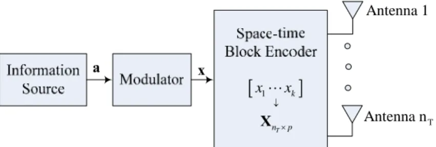
Figure 2.3 Space-time coded transmitter...16

Figure 2.4 Space-time block coded transmitter...16

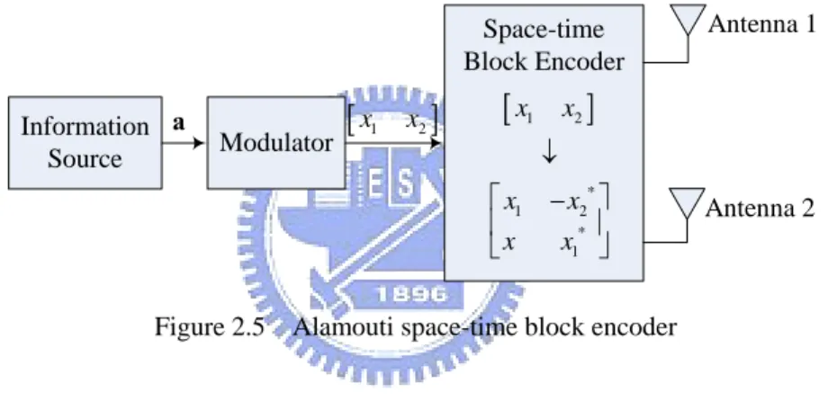
Figure 2.5 Alamouti space-time block encoder...18

Figure 2.6 Trellis description for a 4-state space-time trellis codes with

2 transmit antennas and 4-PSK signal constellation...20

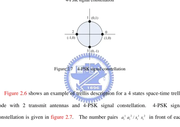
Figure 2.7 4-PSK signal constellation...21

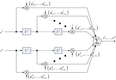
Figure 2.8 Encoder structure of space-time trellis codes...22

Figure 2.9 A trellis example with 4 states...25

Figure 3.1 Equivalent discrete baseband system...30

Figure 3.2 Tapped delay line model of the channel...30

Figure 3.3 Linear equalizer...32

Figure 3.4 Decision-feedback equalizer...33

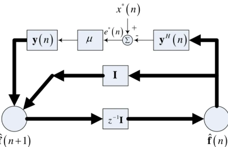
Figure 3.5 Signal-flow graph representation of the LMS algorithm...38

Figure 3.6 Transmitter with encoder and interleaver...40

Figure 3.7 Separate equalization and decoder...40

Figure 3.9 Equalizer block in turbo equalizer...42

Figure 4.1 Transmitter of a space-time trellis coded system...46

Figure 4.2 Squared rooted raised cosine filter with rolloff factor 0.5 and

truncated to be length 13...50

Figure 4.3 Packet format. ...51

Figure 4.4 Transmitter of a space-time trellis coded system...53

Figure 4.5 Equalizer block diagram of a space-time trellis coded

system... ...54

Figure 4.6 Equalizer structure for one receive antenna...55

Figure 4.7 Equalizer structure for two receive antennas...58

Figure 5.1 SER for 2 transmit antennas and 1 receive antenna and

STTC with 32 states...64

Figure 5.2 BER for 2 transmit antennas and 1 receive antenna and

STTC with 32 states...64

Figure 5.3 SER for 3 transmit antennas and 1 receive antenna and

STTC with 32 states...65

Figure 5.4 BER for 3 transmit antennas and 1 receive antenna and

STTC with 32 states...66

Figure 5.5 SER for 4 transmit antennas and 1 receive antenna and

STTC with 32 states...67

Figure 5.6 BER for 4 transmit antennas and 1 receive antenna and

STTC with 32 states...67

Figure 5.7 SER for 2 transmit antennas and 2 receive antenna and

STTC with 32 states...68

Figure 5.8 BER for 2 transmit antennas and 2 receive antenna and

Figure 5.9 SER for 3 transmit antennas and 2 receive antenna and

STTC with 32 states...70

Figure 5.10 BER for 3 transmit antennas and 2 receive antenna and

STTC with 32 states...70

Figure 5.11 SER for 4 transmit antennas and 2 receive antenna and

STTC with 32 states...71

Figure 5.12 BER for 4 transmit antennas and 2 receive antenna and

STTC with 32 states...71

Figure 5.13 BER for different interleaver sizes at 5th iteration with 2

transmit antennas and 1 receive antenna and STTC with 32

states...73

Figure 5.14 SER for different interleaver sizes at 4th iteration with 2

transmit antennas and 1 receive antenna and STTC with 32

states...73

Table Content

Table 4.1 Generator sequences of 32 states and 2, 3 and 4 transmit

antennas...47

Table 4.2 Generator sequences of different state numbers for 2 transmit

Chapter 1 Introduction to MIMO Systems

CHAPTER

1

Introduction to MIMO Systems

The demands for high data rate transmission are increasing rapidly recently. But, the traditional approaches to increase data rate, such as increasing bandwidth, or increasing transmission rate, are becoming impractical due to the limited resource. This leads to considerable effort in finding and developing new approaches in addition to the two aforementioned approaches.

A popular approach is to develop a multiple-input-multiple-output (MIMO) system. In this chapter, we will show how the advantages are obtained from the MIMO system by deriving the fundamental capacity of MIMO channels and comparing it to that of the traditional single-input-single-output (SISO) channels.

At the end of this chapter, we will introduce the motivation of this work and the organization of this thesis.

1.1 MIMO Channel

1.1.1 MIMO Channel Model

Assuming a MIMO channel with n transmit antennas and _T n receive _R

antennas, and the path between each antenna is frequency-flat, then we can express this system as:

Chapter 1 Introduction to MIMO Systems = + r Hx n (1.1) where ₁ R T n r r ⎡ ⎤ = ⎣ ⎦

r is the n_R× received vector, 1 ₁

T T n x x ⎡ ⎤ = ⎣ ⎦ x is the 1 T n × transmitted vector, ₁ R T n n n ⎡ ⎤ = ⎣ ⎦

n is the n_R× additive noise vector. 1

H is the n_R× fading matrix of the form: n_T

11 1 1 T R R T n n n n h h h h ⎛ ⎞ ⎜ ⎟ = ⎜ ⎟ ⎜ ⎟ ⎝ ⎠ H … (1.2)

Let the total transmitted power be constrained to P , regardless of the number of

transmit antennas nT. The power can be represented as

( _xx)

P=tr R (1.3)

where tr i denotes the trace obtained as the sum of diagonal elements, and ( ) R _xx

denotes the covariance matrix obtained by:

{ }

H

xx =E

R xx (1.4)

where E i

{ }

denotes expectation operation. It is common to consider the transmitted signals to be zero mean independent identically distributed (i.i.d.) Gaussian variables. Let us consider the case when transmitted power is split into nT

parts evenly and distributed to nT transmit antennas, then equation (1.4) can be

rewritten as T xx n T P n = R I (1.5) where T n

I is the n_T×n_T identity matrix.

For normalization purposes, we assume that the received power for each of nR

receive antennas is equal to the total transmitted power P. Thus we obtain a normalization constraint for the elements of H as

Chapter 1 Introduction to MIMO Systems 1 x T n x 1 r R n r 11 h 1 T n h 1nR h T R n n h

Figure 1.1 MIMO channel with nT transmit antennas and nR receive antennas

2 1 , 1, , T n ij T R i h n j n = = = …

∑

(1.6)

This system is shown in figure 1.1.

1.1.2 MIMO Channel Capacity

Before we start to derive the channel capacity of MIMO channels, we first review the Shannon’s third theorem [17], the information capacity theorem, as a reminder:

The information capacity of a continuous channel of bandwidth B hertz,

perturbed by additive white Gaussian noise of power spectral density N₀/ 2 and limited in bandwidth to B, is given by

2

0

log 1 Pr bits per second

C B

N B

⎛ ⎞

= _⎜ + _⎟

⎝ ⎠ (1.7)

where Pr represents the received signal power.

Let N B₀ =σ_n2 be the total power of the noise, we rewrite the capacity formula as:

2 2

log 1 r bits per second

n P C B σ ⎛ ⎞ = _⎜ + _⎟ ⎝ ⎠ (1.8)

Chapter 1 Introduction to MIMO Systems

singular value decomposition (SVD) theorem [4], any n_R× matrix H can be n_T

decomposed as:

H

=

H UDV (1.9)

where D is an n_R× non-negative and diagonal matrix, n_T U and V are n_R× n_R

and n_T× unitary matrices, respectively. The diagonal elements of D are the n_T

non-negative square roots of the eigenvalues of HH . Furthermore, the column H

vectors of U are the eigenvectors of HH , and the column vectors of H V are the eigenvectors of H H . The non-negative square roots of the eigenvalues of H HH H

are also referred to as the singular values of H . We denote λ_i as the i th element on the diagonal of D , and then we have the following equations:

H i

λ

=

HH y y (1.10)

where y is an eigenvector corresponding to eigenvalue λ_i By unitary matrices, we imply the following equations exist:

H H = = UU I VV I (1.11)

Substituting (1.9) into (1.1), and multiplying both sides by U , we can rewrite H

equation (1.1) as: H H H H H H = + = + U r U UDV x U n DV x U n (1.12)

Introducing the transformations blow ' ' ' H H H = = = r U r x V x n U n (1.13)

we obtain an equivalent channel model:

'= '+ '

r Dx n (1.14)

We say that equation (1.14) is equivalent to equation (1.1) is because V and U

Chapter 1 Introduction to MIMO Systems

D with respect to different basis.

Due to the diagonal property of D , each element in r' can be expressed as: ' ' ' , 1, 2,

i i i R

r = λ x +n i= n (1.15)

If rank( )H =γ , which also means rank(HHH)=γ , then λ_i ≠ for 0 i=1, 2, γ and 0λ_i = for i= +γ 1, n_R . Rewrite equation (1.13) and apply the property above leads to:

' ' ; 1, ' ; 1, i i i i i i R r x n i r n i n λ γ γ = + = = = + (1.16)

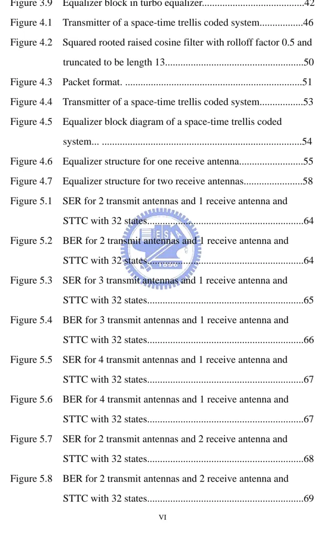
This new equivalent model is shown in figure 1.2

TX RX 1 λ γ λ 0 0 1' x ' xγ 1' x_γ+ ' T n x 1' r ' rγ 1' r_γ+ ' R n r

Figure 1.2 Equivalent MIMO channel after SVD

We have changed the system in figure 1.1 into figure 1.2. From figure 1.2, we see that the original MIMO channel can be expressed as γ parallel equivalent SISO channels, and each SISO channel capacity can be directly computed using the Shannon capacity formula reviewed in equation (1.8). From this viewpoint, the capacity of MIMO channel is now easily obtained by summing all the equivalent SISO channel capacities since they are parallel:

Chapter 1 Introduction to MIMO Systems

2 2

1

log 1 ri bits per second

i i P C B γ σ = ⎛ ⎞ = _⎜ + _⎟ ⎝ ⎠

∑

(1.17)

where P denotes _ri the received signal power of 'r , and _i σ_i2 denotes the noise power of n_i' . P can be obtained using following equations under our _ri

normalization constraint (1.6) ' ' ' ' ' ' ' ' ( ) ( ) ( ) ( ) i i i i i i i i H H i ri r r r r r r x x T P P tr tr tr tr n λ = R = U R U = R = HR H = (1.18)

Thus, the channel capacity can be written as

2 2

1

2 2

1

log 1

log 1 bits per second

i i i T i i i T P C B n P B n γ γ λ σ λ σ = = ⎛ ⎞ = _⎜ + _⎟ ⎝ ⎠ ⎛ ⎞ = _⎜ + _⎟ ⎝ ⎠

∑

∏

(1.19)

Since λ_i ,i= …1, ,γ are the eigenvalues of H

HH , to obtain all λi we have to find the

roots of such equation:

det(λ −I HHH)=0 (1.20)

We can also rewrite equation (1.20) by introducing the roots into the equation:

1 ( i) 0 i γ λ λ = − =

∏

(1.21)

Therefore, we can equal these two equations as blow:

1 det( H) ( i) i γ λ λ λ = − =

∏

− I HH (1.22) Substituting 2 T n P σ

− for λ in (1.22), and multiplying both sides a constant, we get

2 2 1 det( H) (1 i ) T i T P P n n γ _λ σ = σ + =

∏

+ I HH (1.23)

The purpose of doing this is to write the channel capacity formula in(1.19) as

2 2 log det H T P C B nσ ⎛ ⎞ = _⎜ + _⎟ ⎝I HH ⎠ (1.24)

1.1.3 Antenna Numbers versus Capacity

Chapter 1 Introduction to MIMO Systems

determining the capacity. It represents the equivalent parallel SISO channel number. Since H is a n_R× matrix, the rank of H ,n_T γ , will always be less or equal to

min(n n_R, _T). If n_R ≤n_T, the equivalent parallel SISO channel number of the MIMO channel is less or equal to the transmit antenna number. If n_T ≤n_R, the equivalent parallel SISO channel number of the MIMO channel is less or equal to the receive antenna number. It is often a fallacy to think that more antennas there are, more equivalent SISO channels we must have. The fact is: it depends on the rank of the channel. A 3-to-2 MIMO system may give less equivalent SISO channels than a 2-to-2 MIMO system. But for full-rank channels defined as the cases

min(n n_R, _T)

γ = , of course, more antennas give more capacity. Therefore, a full-rank channel is always considered as a good channel for a MIMO system.

1.1.4 MIMO Capacity over Frequency-Selective Channels

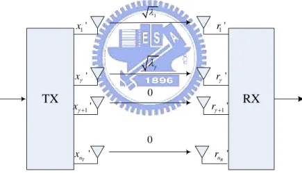
In this section, we consider the capacity of an OFDM-based MIMO channel, and then extend it to general frequency-selective channel capacity. For a K-point OFDM-based system, channel can be considered as K parallel subchannels. If K is large enough, then each subchannel can be approximated as frequency-nonselective. Therefore, a frequency-selective MIMO channel in an OFDM-based system can be approximated as K frequency-nonselective MIMO subchannels if K is large enough as illustrated in figure 1.3. The instantaneous channel capacity of such system is given in [5] as 2 1 log det( ( ) K k k k H k B C SNR K = ⎡ ⎤ ≅

∑

_⎣ I+ H ⋅ H _⎦ (1.25)

where _Hk _{represents the}

th

k subchannel which is a nR×nT matrix, and k

SNR represents the Signal-to-Noise Ratio of the kth subchannel at the receive antenna, and B is the bandwidth of the overall channel.

Chapter 1 Introduction to MIMO Systems

Frequency-selective

Approximately Frequency-nonselective

Figure 1.3 Subchannel of OFDM systems

By comparing equations (1.25) and (1.24), it is not difficult to see that this formula is simply to sum the capacities over the K frequency-nonselective subchannels. The derivation seems plausible; however, it is an approximation because we approximate each subchannel to be frequency-nonselective. To derive the exact formula instead of the approximation, Riemann integral theorem can be applied. That is, when K is approaching to infinite, all subchannels (with the bandwidth B

K ) become frequency-nonselective. The summation in (1.25) becomes integration, and we obtain the exact MIMO frequency-selective channel formula:

(

1

)

2

0 log det ( ) ( ) ( ) ( ) bits per second

B _H

xx nn

C=B

∫

_⎣⎡ I+H f S f H f S − f ⎤_⎦df (1.26) where S_xx( )f represents power spectrum matrix of x at frequency f obtain by

{ }

( )f =FT

S R , and H( )f is the frequency response of the MIMO channel at frequency f .

Chapter 1 Introduction to MIMO Systems

1.2

Introduction to Receivers for MIMO Channel

There are many different transmitting schemes for MIMO systems. The Space-time trellis code is a well-known transmitting scheme which introduces diversity and coding gain. However, as the transmission bandwidth increases beyond the coherent bandwidth of the channel, ISI becomes a major performance-limiting impairment. Equalization becomes indispensable. The theory of equalization for single-input single-output channels has been well-developed. Different criteria and algorithms such as MMSE, BCJR, LMS and RLS are applied to obtain a variety of equalizers. In the recently years, the techniques of turbo equalization are proposed and shown to provide much better performance than the tradition receiving schemes in which the equalization and the decoding are conducted separately. The turbo equalization scheme performs equalization and decoding in an iterative manner and obtains the performance near the Shannon limit.

When MIMO channels are considered, these design criteria and algorithms for the SISO systems remain valid and effective. However, due to the nature of MIMO channel, some modifications or extra effort have to be made. Trellis-based equalizers suffer from the heavy computational complexity. This problem can be mitigated by the use of several techniques such as prefiltering [25] and in-phase/quadrature-phase detection [26]. Filter-based equalizers are low-complexity alternatives. With known channel state information (CSI), MMSE criterion can be derectly applied to the filter-based equalizer as it does in [23] for SISO channels. Without the CSI, MMSE solutions can be approached by the adaptive algorithms such as LMS and RLS as it does in [21] for SISO channels.

In this thesis, the channel state information is assumed to be unknown at the receiver, and we apply adaptive algorithm directly to the equalizer. This structure

Chapter 1 Introduction to MIMO Systems

can be deemed as the MIMO version of the one in [21].

1.3

Motivation

Achieving high bit rates over bandlimited wireless channels makes many applications possible. The use of multiple-antennas brings a bandwidth efficient solution while achieving high bit rate at the same time. The fundamental phenomenon which makes reliable wireless transmission difficult is the multipath fading. Therefore, to overcome this phenomenon is especially important. For some applications, the receivers are also required to be small and power efficient. Thus, a simple receiver structure is attractive. However, the equalization for MIMO channels is generally considered impractical due to the heavy computational complexity. In this thesis, our goal is to develop a low-complexity turbo equalizer for broadband MIMO systems.

1.4

Organization

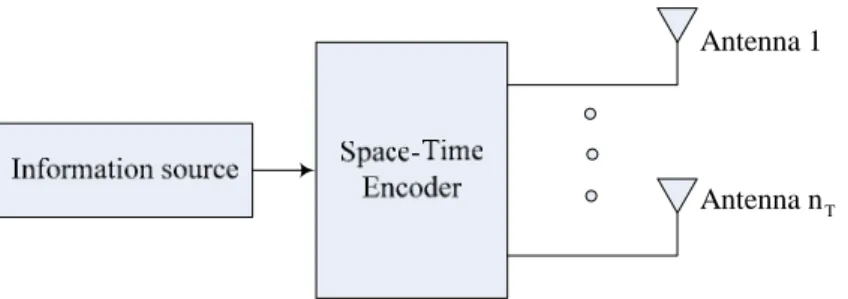
This thesis is organized as follows. Chapter 2 introduces the space-time trellis codes, and its advantages over single-input-single-output trellis codes. The encoding structure and the decoding algorithm are addressed in details. Chapter 3 is the equalizer overview. The filter-based equalizer is the candidate of our design and thus is the main topic of this chapter, too. The ideal of turbo equalization is introduced in chapter 3. In chapter 4, we propose the receiver in combination of the topics in chapter 2 and 3. In this chapter, the details of the receiver are given, including equalization, decoding, interleaving, mapping, and demapping. In chapter 5, we show the simulation results of our proposed system, and some comparison of the systems. Chapter 6 is the conclusion we make on the simulation results and comparisons.

Chapter 2 Space-Time Trellis Codes

CHAPTER

2

Space-Time Trellis Codes

In chapter 1, we have shown the capacity a MIMO channel, but no system implementation has been mentioned. In this chapter, we will introduce the Space-Time Codes which is one approach to take advantages of MIMO channel and provide high data rate or high link quality. Space-time codes have a variety of different structures, each of them has their one advantages and disadvantages. In this chapter, we will first introduce briefly the three diversities commonly used in communication systems. Then we move on to space-time codes which may combine several of the three diversities. The famous space-time block codes will be briefly introduced, and then we focus on the space-time trellis codes which are the channel codes we used in our proposed system in chapter 4.

2.1 Diversity Techniques

Many channels, especially wireless channels, suffer from attenuation due to destructive addition of multipaths in the propagation media and due to the interference from other users. Severe attenuation makes it impossible for the receiver to determine the transmitted signal unless some less-attenuated replica of the transmitted signal is provided to the receiver. This resource is called diversity and it is an

Chapter 2 Space-Time Trellis Codes

important contributor to reliable wireless communications. According to the domain where diversity is introduced, there are three categories of diversity: time diversity, frequency diversity, space diversity.

2.1.1 Time Diversity

The replicas of transmitted signals are provided to the receiver in the form of redundancy in time domain. Identical messages are transmitted in different time slots, and the receiver would receive several uncorrelated fading signals. To be uncorrelated, the time separation between identical messages must be at least the coherent time of the channel. The definition of the coherent time is the period over which the channel fading process is correlated. In many systems, redundancy in time domain is introduced by the error control coding (ECC), and an interleaver is placed after error control coding to provide time separation greater than the coherent time. However, in the receiver, deinterleaving process introduces message delay. For slow fading channels, a larger interleaver is required to exceed the coherent time, and therefore, a larger message delay is introduced. This drawback may be vital to some delay-sensitive applications, especially voice applications. Another drawback of this scheme is that there will be a certain bandwidth efficiency loss due to the redundancy in time domain.

2.1.2 Frequency Diversity

The replicas of transmitted signals are provided to the receiver in the form of redundancy in frequency domain. The frequency separation is required to be at least the coherent bandwidth to obtain uncorrelated fading replicas in the receiver. The definition of the coherent bandwidth is similar to the coherent time: the frequency span over which the channel fading property is uncorrelated. Several mature

Chapter 2 Space-Time Trellis Codes

communication systems introduce the frequency diversity to increase the data rate or improve the link quality. Spread spectrum is one example, this technique includes direct sequence spread spectrum (DSSS), frequency hopping, multicarrier modulation, and CDMA systems. A combination of error-control coding and OFDM can also be considered as frequency diversity, because the time diversity provided by ECC has been transferred into frequency domain by OFDM modulator. These techniques use bandwidths that are far more than enough just to provide frequency diversity, thus, like time diversity, it induces a loss in bandwidth efficiency due to the redundancy introduced in frequency domain.

2.1.3 Space Diversity

The replicas of transmitted signals are provided to the receiver in the form of redundancy in spatial domain. It is typically implement using multiple antennas or antenna arrays arranged in space in a certain manner. Therefore, space diversity is also called antenna diversity. The space separation between antennas is required to be at least the coherent distance. Usually, a few wavelengths are enough for the antennas to experience different fadings. One advantage of this technique is that unlike time and frequency diversity, it doesn’t suffer from the loss in bandwidth efficiency. This advantage makes it very attractive to high data rate wireless communications.

2.1.4 Transmit and Receive Diversity

We can further classify space diversity into receive diversity and transmit diversity depending on where the multiple antennas are applied. The receive diversity is adapted in a variety of mobile communication systems with the aim to both suppress co-channel interference and minimize the fading effects. It is reasonable to apply

Chapter 2 Space-Time Trellis Codes

receive diversity at the base station for uplink (from mobiles to base stations) communication because the power requirement and the dimension requirement are easier to meet compared with mobile devices. For example, in GSM systems, multiple antennas are used at the base station to create uplink receive diversity, compensating for the relatively low transmission power from the mobile. For downlink (from base station to mobiles), it is much more difficult to apply receive diversity at the mobiles. Firstly, placing multiple antennas in a portable mobile device is against the public favor in a smaller device. Secondly, multiple antennas mean more power consumption which is also against the public favor in a power-saving device. Therefore, transmit diversity is more adequate for the downlink communication.

However, in contrast to receive diversity which is widely applied in mobile systems, transmit diversity has gained little attention and is less understood. The reason is that it is more difficult to exploit transmit diversity, and the difficulty is because the transmitted signals are mixed up before they arrive the receiver. Therefore, the receiver requires extra signal processing to separate the transmitted signals before the transmit diversity can be exploited. This signal processing is not always perfect, and may suffer from performance loss. In the next session, we will introduce a transmit diversity technique called “Space-Time Codes”, and in Chapter 4, we will propose a signal processing to separate the transmitted signals.

2.1.5 Combine Different Diversity

Not all forms of diversity can be available at all times. To obtain diversity, the resources providing redundancies must be uncorrelated. Otherwise, you simply obtain the same information twice. For example, in slow fading channels, time diversity is not an option due to large coherent time. When delay spread is small,

Chapter 2 Space-Time Trellis Codes

frequency diversity is not an option due to large coherent bandwidth. When the platform is a small mobile device, space diversity is not suitable due to limited dimensions. Nevertheless, combining different diversities will improve the data rate or link quality if they are available. Transmit diversity and receive diversity can also be combined to provide more advantages.

2.2 Space-Time Coding

In 1993, Wittneben proposed a delay diversity scheme [6]. This scheme transmits the same information from both antennas but with a delay of one symbol interval as shown in figure 2.1. The effect of this process is to introduce an artificial multipath channel to the receiver which changes a narrowband purely frequency-nonselective fading into a frequency-selective fading channel. With this multipath channel, the receiver can utilize a trellis-based equalizer and gain performance improvement from it. In [7], it was shown that the use of a maximum-likelihood sequence estimator at the receiver is capable of providing dual branch diversity.

Information source Mapper

Delay Ts

Chapter 2 Space-Time Trellis Codes

Figure 2.2 Delay diversity transmitter

This framework is identical to figure 2.2 where the channel code is a repetition code with code rate 1

2

R= . In this structure, it is natural to ask if it is possible to design a channel code that is better than repetition code in order to improve performance further. The answer is yes, and we use the term “Space-Time Codes” to refer to these channel codes. In space-time coding, the delay element before antenna unit is removed, and the structure is shown in figure 2.3. Coding is performed in both spatial and temporal domains to introduce correlation between signals transmitted from various antennas at various time periods. Space-time coding can achieve transmit diversity over spatially uncoded systems without sacrificing the bandwidth. There are various approaches in coding structures, including space-time block codes (STBC), and space-time trellis codes (STTC).

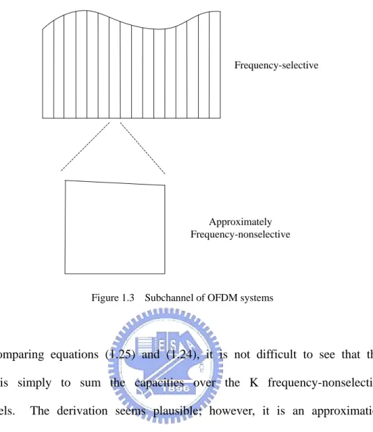
Antenna 1

T

Antenna n

Chapter 2 Space-Time Trellis Codes Antenna 1 T Antenna n

[

1

]

T k n p x x ↓ × X x a

Figure 2.4 Space-time block coded transmitter

2.2.1 Space-Time Block Codes

Space-time block codes operate on a block of input symbols producing a matrix output whose columns represent time and rows represent antennas. Their key feature is the provision of full diversity with extremely low encoder/decoder complexity under frequency-nonselective channels. The space-time block code system is shown in figure 2.4. Assuming nT antennas are used, and p symbols

per antenna are used to convey k uncoded symbols. The code rate is given by k

R p

= (2.1)

To describe the space-time block codes, we use the transmission matrix X which is a nT×p matrix. The element of X in the ith row and jth column,

, , 1, , , 1, ,

i j T

x i= … n j= … p represents the signals transmitted from the antenna i at time j.

The key property of this system is the orthogonality between the sequences generated by the different transmit antennas. This feature was generalized in [8] to an arbitrary number of transmit antennas by applying the theory of orthogonal designs. It is also shown in [8] that to achieve full transmit diversity, the code rate of a space-time block code must be less than or equal to one, R≤1 which requires an bandwidth expansion of 1

R.

Chapter 2 Space-Time Trellis Codes

modulated symbols x1,…,xk and their conjugates

* * 1, , k

x … x . To achieve the orthogonality, X must satisfy the following equation:

(

2 2

)

1 T H k n c x x ⋅ = + X X I (2.2) where c is a constant, _XH

is the Hermitian of X and

T

n

I is an nT×nT identity

matrix. Through the orthogonal designing, the signal sequence from any two transmit antennas are orthogonal. This property enables the receiver to decouple the signals transmitted from different antennas and consequently, a simple maximum likelihood decoding, based only on linear processing of the received signals.

Antenna 1 Antenna 2 Modulator Information Source Space-time Block Encoder

[

1 2

]

* 1 2 * 1 x x x x x x ↓ ⎡ − ⎤ ⎢ ⎥ ⎣ ⎦

[

x1 x2

]

a

Figure 2.5 Alamouti space-time block encoder

The Alamouti code [9], was the first and the most famous space-time block code. It is achieve a full diversity gain using two transmit antennas and a simple maximum-likelihood decoding algorithm. The transmission matrix is given by

* 1 2 * 2 1 x x x x ⎡ − ⎤ = ⎢ ⎥ ⎣ ⎦ X (2.3)

Figure 2.5 shows an encoder structure for Alamouti code. It is easy to see that the transmit sequence from antennas one and two are orthogonal,

1 2 * * 1 2 2 1 0

x x x x

⋅ = − =

x x (2.4)

The decoding of space-time block codes was based on maximum likelihood algorithm. Assuming one receive antenna and perfect channel state information (CSI) is know at the receiver. Using Alamouti code as an example, the maximum

Chapter 2 Space-Time Trellis Codes

likelihood decoder choose a pair of signals ( ,x xˆ ˆ1 2) from the signal modulation

constellation to minimize the distance metric

( )

(

)

2 2 *

1, 1 1ˆ 2ˆ2 2, 1 2ˆ 2 1ˆ *

d r h x +h x +d r h x +h x (2.5)

With some simple transformation, the decision rule can be derived as

( ) ( ) 1 2 2 1 1 1 ˆ 2 2 2 2 ˆ ˆ arg min ,ˆ ˆ arg min ,ˆ x x x d x x x d x x ∈ ∈ = = S S (2.6)

where S is the set of all possible modulated symbol pairs ( ,x xˆ ˆ1 2) and * * 1 1 1 2 2 * * 2 2 1 1 2 x h r h r x h r h r = + = + (2.7)

The decision rules derivation can be extended to other cases with other number of receive antennas, and they can be found in [8].

Space-time block codes can achieve a maximum possible diversity advantage with a simple decoding algorithm. It is very attractive because of its simplicity. However, no coding gain can be provided by space-time block codes, and also, non-full rate space-time block codes can introduce bandwidth expansion.

2.2.2 Space-Time Trellis Codes

Space-time trellis codes operate on one input symbol at a time producing a sequence of vector symbols whose length represents antenna number. Like traditional trellis coded modulation (TCM) for the single-antenna channel, space-time trellis codes provide coding gain. Since they also provide full diversity gain, their key advantage over space-time block codes is the provision of coding gain. Space-time trellis codes are nowadays widely discussed as it can simultaneously offer a substantial coding gain, spectral efficiency, and diversity improvement on flat fading channels. The case for frequency-selective channels are studied in [13][18], and the conclusion of [13] is that the frequency-selective channel doesn’t affect the diversity

Chapter 2 Space-Time Trellis Codes

provided by space-time trellis codes. However, compared with space-time block codes, this code is far more difficult to design, and also requires a computationally intensive encoder and decoder. The key development was done by Tarokh, Seshadri and Calderbank in 1998 [1], and some other improved development was done in

[10][11][12]. In next session, we will talk about it in detail.

2.3

Space-Time Trellis Codes

2.3.1 Trellis description

The space-time trellis codes are described by trellis structures. Considering a space-time trellis coded M-PSK modulation with nT transmit antennas. The

encoder takes a group of m=log2M information bits at time t given by

(

1

)

, , m

t = at at

a … (2.8)

and produces a group of mnT coded bits

(

)

(

)

(

1 1

)

,1, , , , , ,1 , , , T T n n t = ct ct m ct ct m c … … … (2.9) Each

(

,1, , ,T

)

, 1, , i i t t n T

c … c i= … n are mapped into symbol i t

x , and thus ct is mapped

into a group of nT symbols given by

(

1

)

, , nT

t = xt xt

x … (2.10)

where each xti ,i= …1, ,nT is an M-PSK modulated signal. At each time t ,

depending on the state of the encoder and the input bits, a transition branch is chosen. On the trellis, each branch transition is labeled of

(

1

)

, , nT

t t

x … x which means the transmit antenna i is used to send symbol i

t

x , and all these transmissions are simultaneous.

Chapter 2 Space-Time Trellis Codes

Figure 2.6 Trellis description for a 4-state space-time trellis codes with 2 transmit antennas and 4-PSK signal constellation 0 1 2 3 (1,0) (0,1) (-1,0) (0,-1)

Figure 2.7 4-PSK signal constellation

Figure 2.6 shows an example of trellis description for a 4 states space-time trellis code with 2 transmit antennas and 4-PSK signal constellation. 4-PSK signal constellation is given in figure 2.7. The number pairs 1 2 1 2

/

t t t t

a a x x in front of each state are the labels of each branch transition starting from that state. The left-most number pair is corresponding to the top-most branch transition of the state. As an illustration, if the encoder is in the second state at time t, the input at this time is 11, then the encoder chooses the branch transition from the second state to the fourth state. This branch transition is labeled 11/13 which means antennas (1,2) will transmit the symbol (1,3) respectively.

The trellis is a representation which can fully describe the space-time trellis codes. However, it is common to describe the space-time trellis codes as generator descriptions in the encoders.

Chapter 2 Space-Time Trellis Codes

(

1 1

)

1 1 ,1, , ,T v v n g … g

(

1 1

)

0,1, , 0,nT g … g

∑

(

1 1

)

1,1, , 1,nT g … g

(

0,1, , 0,T

)

m m n g … g

(

1,1, , 1,T

)

m m n g … g

(

m,1, , m,T

)

m m v v n g … g 1 c m c 1 , , nT x … x

Figure 2.8 Encoder structure of space-time trellis codes

2.3.2 Generator Description

The encoder structure of space-time trellis code is shown in figure 2.8. The k-th input sequence k=

(

₀k, , k,

)

, 1, ,

t

a a k= m

a … … … is fed into the k-th shift register and multiplied by a generator sequence gk, k=1,…,m. The multiplier outputs from all shift registers are added up in modulo-M to give the encoder output x=(x₀,…,x_t,…). The generator sequence gk, k=1,…,m is of the form:

(

0,1, , 0,

) (

, , ,1, , ,

)

, 1, k k T k k T k k k n v v n g g g g k m ⎡ ⎤ =_{⎣ ⎦} = g … … … … (2.11)

The total memory order of the encoder, denoted by v is given by

1 m k k v v = =

∑

(2.12)

where v_k, k= …1, ,m is the memory order for the k-th lane of shift register, and is given by 2 1 log k v k v M ⎢ + − ⎥ = ⎢ ⎥ ⎣ ⎦ (2.13)

Chapter 2 Space-Time Trellis Codes , 1 0 mod , 1, , k v m i k k t j i t j T k j x g a− M i n = = =

∑∑

= … (2.14)

As an example, let us consider a scheme of 4-state space-time trellis coded QPSK system with 2 transmit antennas and the generator sequences are

( ) ( ) ( ) ( ) 1 2 02 , 20 01 , 10 = ⎡_⎣ ⎤_⎦ = ⎡_⎣ ⎤_⎦ g g (2.15)

The resulting trellis structure is shown in figure 2.6, which is the same as the one we use as an example in the previous session.

2.3.3 Design Criteria

For a given encoder structure, a set of encoder coefficients is determined by minimizing the error probability. It is shown in [1] that the error rate for slow fading channels, the upper bound is depend on the value of r which is the rank of codeword distance matrix _{A X X}

( )

_,ˆ _{. It can be obtained by utilizing the codeword difference} matrix _{B X X}

( )

_,ˆ

( ) ( ) ( )

_,ˆ = _,ˆ ⋅ H _,ˆ

A X X B X X B X X (2.16)

where _Xˆ _{is the erroneous decision mad by decoder when the transmitted sequence} was in fact X. Therefore, in order to minimize the error probability, we have two different criteria:

z Rank & determinant criteria: If rn_R <4, the minimum rank r over all pairs of distinct codewords should be maximized. Also, the determinant of _{A X X}

( )

_,ˆ along the pairs of distinct codewords with the minimum rank should maximized, too.

z Trace criteria: If rn_R ≥4, the minimum trace of _{A X X}

( )

_,ˆ _{among all pairs of} distinct codewords should be maximized.

Chapter 2 Space-Time Trellis Codes

These criteria were derived and summarized in [1] along with the criteria for fast fading channels. The above criteria was referred to as the Tarokh/Seshadri/Calderbank (TSC) codes. An improved criterion was proposed and referred to as the Baro/Bauch/Hansmann (BBH) codes [14].

2.4 Decoding Algorithm

2.4.1 Maximum A posterior Probability (MAP) Decoder

To recover the information bits at the receiver, it is natural to choose a receiver that achieves the minimum probability of error P a( _k ≠aˆ_k) where aˆ_k is the decision of k-th information bit. It is well known that this is achieved by setting aˆ_k to the value which maximizes the a posteriori probability (APP) P a( _k =aˆ_k y) given the received sequence y, i.e.

ˆ ˆ arg max ( ˆ ) k k k k c a = P a =a y (2.17)

The algorithms that achieve this task are commonly referred to as maximum a posteriori probability (MAP) algorithms.

When probabilities are concerned, it is often convenient to work with log-likelihood ratios (LLRs) rather than actual probabilities. The LLR for a variable

k a is defined as ( 1) ( ) ln ( 0) k k k P a L a P a = = = (2.18)

The LLRs contains the same information as the probabilities P a( _k =1) or P a( _k =0). In fact, the sign of L a( _k) determines whether P a( _k =1) is larger than P a( _k =0) or it is on the contrary. Therefore, by using this property of LLRs, the decision rules (2.17) can be further written as

1, ( | ) 0 ˆ 0, ( | ) 0 k k k L a a L a ≥ ⎧ = ⎨ _< ⎩ y y (2.19)

Chapter 2 Space-Time Trellis Codes

The main problem of the MAP approach is that the APPs calculation is computation-intensive. To show this, we use Bayes’ rule and the theorem of total probability [15] on P a( _k =aˆ_k | )y , and obtain

ˆ ˆ : = : = ( | ) ( ) ˆ ( | ) ( | ) ( ) k k k k k k a a a a P P P a a P P ∀ ∀ = =

∑

=

∑

a a y a a y a y y (2.20)

The computation loading in this equation is too heavy. Therefore we introduce algorithms which require less computation complexity than (2.20).

2.4.2 BCJR Algorithm

This algorithm was proposed in1974 by Bahl, Cocke, Jelinek, and Raviv [16], and is now known as the name “BCJR algorithm” composed of the initials of four authors. This is a algorithm to efficiently compute the APPs of interestP a( _k =aˆ_k| )y .

3 r 2 r 0 r 1 r 3 r 2 r 0 r 1 r

Figure 2.9 A trellis example with 4 states

We denote the pair ( , )i j as the branch transition from state r_i to state r_j. Define a set β of ( , )i j , and each pair in the set is a valid branch transition to the chosen trellis. For example, the trellis in figure 2.9 has the set

( ) ( ) ( ) ( ) ( ) ( ) ( ) ( )

{

00 , 01 , 12 , 13 , 20 , 21 , 32 , 33

}

=

β (2.21)

We also denote sk∈S as the state of the encoder when k-th set of information bits

Chapter 2 Space-Time Trellis Codes

is the memory order of the encoder.

We begin with the computation of the probability that the transmitted sequence path in the trellis contained the branch transition from state ri to state rj when the

-th

k set of information bits is the input, i.e., to compute P s( _k =r s_i, _k+1=r_j | )y . Applying the chain rule for joint probabilities, i.e., P a b( , )=P a P b a( ) ( | ), we can obtain

1 k k+1

( ,_{k k} , ) ( ) P(s ,s | )

P s s ₊ y =P y ⋅ y (2.22)

The left hand side of this equation can be written as

( )

1 1 1 1 1

( ,_{k k} , ) _k, _k , ( , _k ), _k, ( _k , _N)

P s s₊ y =P s s ₊ y …y₋ y y₊ …y (2.23) Applying the chain rules again on (2.23), we obtain the key decomposition

( ) ( )

(

)

( ) ( )

(

)

( )

(

)

( ) 1 1 1 1 1 1 1 1 1 1 1 1 1 1 1 , , , , ( , ) , , ( , ) , ( , ) , , , , k k k k k k k k k k k k k k N k k k k k k k k N k s s s s P s s P s y y P s y y y s y y P s y y P s y s P y y s α γ + β+ + + − + + − − + + + = = y … … … … … (2.24)

It is easy to see that the term α_k( )s_k can be computed from α_k−1( )s_k−1 and

( )

1 1,

k sk sk

γ _{− −} , and therefore it can be extended to a recursive computation:

( ) ( ) ( ) 1 1 1 1 1, k k k k k k k k s S s s s s α α γ − − − − − ∈ =

∑

(2.25)

with initial states α₀( )r₀ =1 and zero for other states. Likewise, the term β_k( )s_k has also a recursive computation formula:

( ) ( ) ( ) 1 1 1 , 1 k k k k k k k k s S s s s s β β γ + + + + ∈ =

∑

(2.26)

with end states βN( )r0 =1 and zeros for other states. The assigned values of α0

( )

s and β_N

( )

s are because an encoder always starts at the zeros state and end at the zero state. For all k, the probability of αk( )sk and βk( )sk must be normalized to 1

which means

( )

( )

2 1 0 2 1 0 1 1 v v k i i k i i r r α β − = − = = =

∑

∑

(2.27)

From (2.25) and (2.26), we know that if we have the knowledge of all

( , 1), 0, , 1

k s sk k k N

Chapter 2 Space-Time Trellis Codes

term γk(s sk, k+1) can be further decomposed into

( , 1) ( 1| ) ( | , 1)

k s sk k P sk sk P yk s sk k

γ ₊ = ₊ ⋅ ₊ (2.28)

With specific state numbers, (2.28) can be written as

(

)

(

) (

)

( ) ( ) , , 1 | , , , 0, , k i j k k i j k k i k j P P y x x i j s r s r i j γ = ₊ = _{= ⎨}⎧⎪ = ⋅ = ∈ ∉ ⎪⎩ a a β β (2.29)

where ai j, represent the set of information bits corresponding to branch transition

from state r_i to state r_j . Usually, the information bits are assumed to be independent identically distributed (i.i.d.), which makes ( ) 1

2 m k P = ⎜ ⎟⎛ ⎞ ⎝ ⎠ a . As for

(

k| k i j,

)

P y x =x term, how to calculate it is dependent on the system. For the simple

system with only one decoder and AWGN channel, this term is simply the pdf. of the noise distribution, i.e.

2 2 2 ( ) 1 ( | ) exp 2 2 k k k k y x P y x σ πσ ⎛ − ⎞ = _⎜− _⎟ ⎝ ⎠ (2.30)

where σ2 _{is the power of the noise. In this thesis, we will propose a turbo equalizer}

system, and this term will be provided by the equalizer.

Our goal is to compute the APPs P a( _k =aˆ |_k y). Since we have derived the formula for P(s ,sk k+1| )y , we can sum the APPs P(s ,sk k+1| )y over all branches that

correspond to a_k =aˆ_k. This idea is actually the theorem of total probability [15].

( )

(

)

( )

(

)

( ) ( ) ( )

( ) ( )

( ) ( ) , , , 1 , : 1 , : 1 , : ˆ | , | , , , i j k i j k i j k k k k i k j i j a a k i k j i j a a k i k i j k j i j a a P a a P s r s r P s r s r P r r r r P α γ β + ∀ ∈ = + ∀ ∈ = + ∀ ∈ = = = = = = = = =

∑

∑

∑

β β β y y y y y (2.31)

Chapter 2 Space-Time Trellis Codes ( ) ( )

( ) ( )

( ) ( ) ( )

( ) ( )

( ) ( ) ( )

( ) ( )

( ) ( )

( ) ( )

( ) , , , , 1 , : 1 1 , : 0 1 , : 1 1 , : 0 , ˆ | , , , i j i j i j i j k i k i j k j i j a k k k i k i j k j i j a k i k i j k j i j a k i k i j k j i j a r r r r P L a a r r r r P r r r r r r r r α γ β α γ β α γ β α γ β + ∀ ∈ = + ∀ ∈ = + ∀ ∈ = + ∀ ∈ = = = =

∑

∑

∑

∑

β β β β y y y (2.32)

The turbo equalizer system will also require the computation of L c( _k =cˆ |_k y), and this is done similarly as follows,

( ) ( )

( ) ( )

( ) ( ) ( )

( ) ( )

( ) ( ) ( )

( ) ( )

( ) ( )

( ) ( )

( ) , , , , 1 , : 1 1 , : 0 1 , : 1 1 , : 0 , ˆ | , , , i j i j i j i j k i k i j k j i j c k k k i k i j k j i j c k i k i j k j i j c k i k i j k j i j c r r r r P L c c r r r r P r r r r r r r r α γ β α γ β α γ β α γ β + ∀ ∈ = + ∀ ∈ = + ∀ ∈ = + ∀ ∈ = = = =

∑

∑

∑

∑

β β β β y y y (2.33)

Chapter 3 Turbo Equalization

CHAPTER

3

Turbo Equalization

For wideband systems, because the bandwidth of the transmitted signals is large and often exceeds the coherent bandwidth of the channel, the channels usually have frequency-selective characteristics. The selectivity in frequency is aroused by the multipath fading channel in which transmission paths have different delays and fadings. This channel can be charactered by a tapped-delay line filter. The objective of an equalizer is to eliminate the distortion induced by the frequency-selective channel. Structures of a variety of equalizers are surveyed in this chapter. The algorithms to derive the optimal filter coefficients are also briefly introduced here. At the end of this chapter, a promising equalization scheme incorporated with the turbo principle is introduced.

3.1 Frequency-Selective Channel

Figure 3.1 shows an equivalent discrete baseband system including transmitter and receiver. Here we focus on channel and equalizer only. The system does not include any coding layer which is commonly found in practical communication systems. To add coding layers into this system is straightforward, that is to replace

Chapter 3 Turbo Equalization

the information source with the coded bits. Information bits a in figure 3.1 is mapped into modulated symbols x according to a chosen modulation. A transmit

filter and a receiver filter are used to meet the spectrum requirement and to mitigate the effect of frequency-selective channel. The objective of the equalizer at the receiver is to recover the symbols x from the output of the receive filter y . The

relation between x and y is

(

)

(

T

)

R

= ∗ ∗ ∗ + ∗

y x g h g n v (3.1)

where ∗ is the operation of convolution. We define a new channel h to be _T

T = T∗ ∗ R h g h g (3.2) and rewrite (3.1) to be T T = ∗ + y h x n (3.3)

where n_T = ∗n v . The h represents the total effect of the transmit filter, channel, _T

and the receive filter. It is the channel that equalizers have to cope with, and can be charactered by the tapped-delay line model as shown in figure 3.2. Thus, channels can be described by the impulse response

(

h_T

[ ]

0 ,…,h L_T

[ ]

)

where L is the channel order. a x d y ˆx ˆa n r h T g gR

Figure 3.1 Equivalent discrete baseband system

∑

[ ]

1

h h

[ ]

2 h L

[ ]

[ ]

0 h

Chapter 3 Turbo Equalization

3.2 Equalizer Overview

3.2.1 Trellis-Based

Due to the tapped delay line model of the channel, we can derive a trellis description for the channel. With this trellis description, the BCJR algorithm we presented in 2.4.2 can also be applied readily to detect the symbols. To apply BCJR algorithm in the equalizer, the initial values of α0( )s0 and βN( )sN need to be

modified according to the property of channels. Usually, the channel starts at the zero state and ends at arbitrary state, which leads to

0 1 , 0 ( ) 0 , 0 ( ) 1 for all i N i i r i r i α β = ⎧ = ⎨ _≠ ⎩ = (3.4)

Or, if the channel was preoccupied by the previous transmission, the value α0( )s0

will be α₀

( )

ri =1 for all i.

This approach of equalization requires the knowledge of channel state information (CSI). This requires another effort in channel estimating, and the accuracy of the estimate will affect the detection performance in a certain level.

However, the problem of an trellis-based equalizer is the complexity. The state number of the equivalent trellis is dependent on the channel order L , the signal constellation M-PSK, and transmit antenna n_T in a MIMO system. It can be calculated by

( )

nT

state number = M L (3.5)

For example, if the transmitter uses 2 transmit antennas and 4-PSK modulation, and the channel order is 5, then we will have a equivalent trellis of state number

( )

₂ 5

4 =1048576. This is a huge number for a decoder to build, not to mention the one with more antennas or with higher constellation. Therefore, this approach is