厚尾分配在財務與精算領域之應用 - 政大學術集成

全文

(1)國立政治大學風險管理與保險學系博士論文. 指導教授：黃泓智. 立. 博士. 政治大. ‧ 國. 學. 厚尾分配在財務與精算領域之應用. ‧. n. al. er. io. sit. y. Nat. Applications of Heavy-Tailed Distributions in Finance and Actuarial Science. Ch. engchi. 博士生：劉議謙. 中. 華. 民. 國. 一. 〇. i n U. v. 撰. 一. 年. 九. 月.

(2) 謝. 誌. 論文終於完成了！非常感謝我的指導教授黃泓智教授，高雄第一科技大學的王昭文教授，以及加拿大滑鐵盧大學的 Ken Seng Tan 教授，沒有這三位教授的大力指導，我相信我是無法完成這本論文的，議謙在此致上最高的感謝之意。另外，還要感謝論文口試委員：俞明德教授、張傳章教授、王儷玲教授以及戴天時教授，口試時給予議謙許多建議及指導，使本論文更加縝密與完整，議謙感恩在心。還有所有教過我的授課老師們，因為有您們的教學，啟發了我許多想法並增. 政治大. 強了我許多觀念，謝謝您們。還要感謝中央大學的楊曉文教授，也就是我碩士班. 立. 的指導老師，感謝楊老師持續願意與我討論許多議題並指導我撰寫投稿文章。. ‧ 國. 學. 在博士班求學期間，幸運獲得 2010-2011 年度「中華扶輪獎學金」，感謝扶輪社的栽培，並謝謝嘉義北區社的照顧。此外，感謝國科會讓我有機會得到「補. ‧. 助博士生赴國外研究」，得以至加拿大滑鐵盧大學向 Ken Seng Tan 教授學習，議. al. er. io. sit. y. Nat. 謙非常感謝。. n. 於風險管理與保險學系就讀的四年間，感謝博士班的永琮學長、芳書學長、. Ch. engchi. i n U. v. 瑞益學長、雅文學姐、尚穎學長、麗如學姐、文彬學長、俞沛學長、士弘學長、志峰、昶翔、耿郎學長、玉鳳學姐、紓婷、可倫、恕銘、柏翰、芳文學姐、筱昀學姐等人，以及碩士班的芫綺、珮娟、慧婷、德全、振格等人，在生活上以及課業上相互扶持，豐富的我博士班苦悶的求學歷程，這是一段非常美好的回憶。最後，感謝我的家人，爸爸、媽媽及姊姊總是全力支持我並給我正面的力量，每每讓沮喪的我馬上又恢復了活力。感謝一路上支持我的親戚朋友們，您們的鼓勵，議謙都會銘記在心，在未來的人生中，議謙會更加努力來回饋社會。. i .

(3) 摘. 要. 本篇論文將厚尾分配（Heavy-Tailed Distribution）應用在財務及保險精算上。本研究主要有三個部分：第一部份是用厚尾分配來重新建構 Lee-Carter 模型（1992），發現改良後的 Lee-Carter 模型其配適與預測效果都較準確。第二部分是將厚尾分配建構於具有世代因子（Cohort Factor）的 Renshaw and Haberman 模型（2006）中，其配適及預測效果皆有顯著改善，此外，針對英格蘭及威爾斯（England and Wales）訂價長壽交換（Longevity Swaps），結果顯示此模型可以支付較少的長壽. 政治大. 交換之保費以及避免低估損失準備金。第三部分是財務上的應用，利用 Schmidt. 立. 等人（2006）提出的多元仿射廣義雙曲線分配（Multivariate Affine Generalized. ‧ 國. 學. Hyperbolic Distributions; MAGH）於 Boyle 等人（2003）提出的低偏差網狀法（Low Discrepancy Mesh; LDM）來定價多維度的百慕達選擇權。理論上，LDM 法的數. ‧. 值會高於 Longstaff and Schwartz（2001）提出的最小平方法（Least Square Method;. y. Nat. al. n. 維度之百慕達選擇權的真值落於此範圍之間。. Ch. engchi. er. io. sit. LSM）的數值，而數值分析結果皆一致顯示此性質，藉由此特性，我們可知道多. i n U. v. 關鍵字：隨機死亡率模型；厚尾分配；長壽交換；百慕達選擇權；多元 Lévy 分配；低偏差網狀法。. ii .

(4) Abstract The thesis focus on the application of heavy-tailed distributions in finance and actuarial science. We provide three applications in this thesis. The first application is that we refine the Lee-Carter model (1992) with heavy-tailed distributions. The results show that the Lee-Carter model with heavy-tailed distributions provide better fitting and prediction. The second application is that we also model the error term of Renshaw and Haberman model (2006) using heavy-tailed distributions and provide an iterative fitting algorithm to generate maximum likelihood estimates under the Cox. 政治大 premiums of longevity swaps 立 and avoid the underestimation of loss reserves for regression model. Using the RH model with non-Gaussian innovations can pay lower. ‧ 國. 學. England and Wales. The third application is that we use multivariate affine generalized hyperbolic (MAGH) distributions introduced by Schmidt et al. (2006) and. ‧. low discrepancy mesh (LDM) method introduced by Boyle et al. (2003), to show how. sit. y. Nat. to price multidimensional Bermudan derivatives. In addition, the LDM estimates are. n. al. er. io. higher than the corresponding estimates from the Least Square Method (LSM) of. v. Longstaff and Schwartz (2001). This is consistent with the property that the LDM. Ch. engchi. i n U. estimate is high bias while the LSM estimate is low bias. This property also ensures that the true option value will lie between these two bounds.. Keywords: Stochastic Mortality Models; Heavy-Tailed Distributions; Longevity Swaps; Bermudan Options; Multivariate Lévy Distributions; Low Discrepancy Mesh.. iii .

(5) Contests Chapter 1. Introduction .................................................................................................. 1 Chapter 2. Heavy-Tailed Distributions ........................................................................ 11 2.1. Introductions of Heavy-Tailed Distributions .................................................... 11 2.2. The Standardization Approaches for Heavy-Tailed Distributions .................... 17 2.3. Estimation Scheme with Standardization .......................................................... 20 Chapter 3. A Quantitative Comparison of the Lee-Carter Model under Different Types of Non-Gaussian Innovations ...................................................................................... 23 3.1. The Lee-Carter Model with Heavy-Tailed Innovations .................................... 23 3.2. Empirical Analysis ............................................................................................ 31 3.3. Conclusions ....................................................................................................... 47. 政治大. Chapter 4. Mortality Modeling with Non-Gaussian Innovations and Applications to the Valuation of Longevity Swaps............................................................................... 49. 立. 4.1. Stochastic Mortality Models with Cox Error Structures ................................... 49. ‧ 國. 學. 4.2. Empirical Analysis ............................................................................................ 55 4.3. Application: The Valuation of Longevity Swaps .............................................. 59. ‧. 4.4. Conclusions and Suggestions ............................................................................ 68. sit. y. Nat. Chapter 5. Pricing High-Dimensional Bermudan Options with Lévy Processes Using Low Discrepancy Mesh Methods ................................................................................ 71. er. io. 5.1. Multivariate Affine Generalized Hyperbolic Distributions .............................. 71 5.2. Low Discrepancy Mesh (LDM) Method ........................................................... 75. n. al. Ch. i n U. v. 5.3. Empirical and Numerical Analyses ................................................................... 79. engchi. 5.4. Conclusions ....................................................................................................... 91 Chapter 6. Conclusions ................................................................................................ 93 Appendix A .................................................................................................................. 97 Appendix B .................................................................................................................. 99 Appendix C ................................................................................................................ 101 Appendix D ................................................................................................................ 103 Appendix E ................................................................................................................ 105 Appendix F................................................................................................................. 107 References .................................................................................................................. 109. iv .

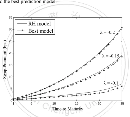
(6) List of Figures Figure 3-1. The Probability Density Functions of Standardized Residuals ................. 26 Figure 3-2. The Pattern of Mortality Indices ............................................................... 27 Figure 3-3. The Probability Density Functions of the First Difference in Mortality Indices .......................................................................................................................... 28 Figure 4-1. Swap Premium Curves for Distinct Level of Risk-Adjusted Parameter  ...................................................................................................................................... 64 Figure 4-2. Probability Density Functions of Present Value of the Losses ................. 67. 立. 政治大. ‧. ‧ 國. 學. n. er. io. sit. y. Nat. al. Ch. engchi. v . i n U. v.

(7) List of Tables Table 3-1. Skewness, Excess Kurtosis and the Jarque-Bera Test ................................ 29 Table 3-2. Goodness-of-fit Measures for the Residuals of the Lee-Carter Model ...... 35 Table 3-3. Goodness-of-fit Tests for the Residuals of the Lee-Carter Model ............. 37 Table 3-4. Goodness-of-fit Tests for the First Difference in Mortality Indices........... 40 Table 3-5. Goodness-of-fit Tests for the First Difference in Mortality Indices........... 42 Table 3-6. Percentile of MAPE of Mortality Projection .............................................. 45 Table 4-1. The Jarque-Bera Test .................................................................................. 51 Table 4-2. Goodness-of-fit Measures for the Number of Deaths ................................ 56 Table 4-3. Goodness-of-fit Tests for the First Difference in Mortality Indices........... 57. 治政 Table 4-5. MAPE of Logarithm of Mortality Projection大 in 1984-2008 (Unit: %) ...... 59 Table 4-6. Goodness-of-fit立 Measures for the Number of Deaths in 1900-2008 .......... 63. Table 4-4. Goodness-of-fit Tests for the Residuals of Cohort Effects ........................ 57. ‧ 國. 學. Table 4-7. Swap Premiums for Different Interest Rates .............................................. 65 Table 4-8. The MTM Values of Longevity Swaps ...................................................... 66. ‧. Table 4-9. The VaR and CTE of the Losses for Different Maturation Times ............. 68 Table 5-1. Descriptive Statistics .................................................................................. 79. Nat. sit. y. Table 5-2. Estimated Parameters for MAVG and MANIG ......................................... 80. er. io. Table 5-3.  and Esscher Parameters  for MAVG and MANIG ........................ 80. al. Table 5-4. Put Option on Single Asset (4 exercise points) .......................................... 85. n. v i n Table 5-5. Put Option on SingleC Asset (8 exercise points) h e n g c h i U .......................................... 86 Table 5-6. Put Option on the Maximum of Two Assets (4 exercise points) ............... 87 Table 5-7. Put Option on the Maximum of Two Assets (8 exercise points) ............... 88 Table 5-8. Put Option on the Maximum of Three Assets (4 exercise points) ............. 89 Table 5-9. Put Option on the Maximum of Three Assets (8 exercise points) ............. 90. vi .

(8) Chapter 1 立 Introduction. 政治大. ‧ 國. 學 ‧. The heavy-tailed distributions have been used in financial field for many years. The scholars of insurance field use these distributions to discuss some problems step. y. Nat. io. sit. by step. First we want to refine existing two mortality models by some heavy-tailed. n. al. er. distributions, and we then price high-dimensional Bermudan options using the low. Ch. i n U. v. discrepancy mesh (LDM) with multivariate affine generalized hyperbolic (MAGH).. engchi. Longevity represents an increasingly important risk for defined benefit pension plans and annuity providers, because life expectancy is dramatically increasing in developed countries. In 2007, exposures to improved life expectancy amounted to $400 billion for pension funds and insurance companies in the United Kingdom and United States (see Loeys et al., 2007). Stochastic mortality models quantify mortality and longevity risks, which makes mortality risk management possible and provides the foundation for pricing and reserving. Among all stochastic mortality models, the Lee-Carter model (LC), proposed in 1992, is one of the most popular choices because of its ease of implementation and acceptable prediction errors in empirical studies. 1 .

(9) Various modifications of the LC model have been extended by Brouhns et al. (2002), Renshaw and Haberman (2003, 2006), Cairns et al. (2006), Li and Chan (2007), Biffis et al. (2010), and Hainaut (2012) to attain a broader interpretation. Cairns et al. (2006) propose a two-factor stochastic mortality model, the CBD model, in which a first factor affects mortality at all ages, whereas a second factor affects mortality at older ages much more than at younger ages. Modeling the number of deaths with the Poisson model, Cairns et al. (2009) classify and compare eight stochastic mortality models, including an extension of the CBD model, with mortality data from England and Wales and the United States. They find that an extension of the CBD model that. 治政大 data best, whereas for the incorporates the cohort effect fits the English and Welsh 立. U.S. data, the Renshaw and Haberman (2006) model (RH), which also allows for a. ‧ 國. 學. cohort effect, provides the best fit (Cairns et al., 2009). In addition to the cohort effect,. ‧. short-term catastrophic mortality events, such as the influenza pandemic in 1918 and. sit. y. Nat. the Tsunami in December 2004, may lead to much higher mortality rates. Using. io. er. empirical data from 1900 to 1983, we find that the residuals in the RH model for England and Wales, France, and Italy exhibit leptokurticity. It is crucial to address. al. n. v i n Ch such mortality jumps in age–period–cohort models. e n gmortality chi U. To the best of our knowledge, Hainaut and Devolder (2008) were the first to. apply α-stable subordinators (infinite-activity, strictly positive, Lévy processes) to model mortality hazard rates. However, in the Lee-Carter model, the first difference of mortality indices may be negative, to reflect mortality improvements. Giacometti et al. (2009) consider both the error distributions of the Lee-Carter model and its mortality index, using the NIG distribution to model mortality for different age groups. They observe that the NIG distributional assumption for the residuals of the Lee-Carter model is better than the Gaussian one for some age groups. To take 2 .

(10) non-Gaussian distributions into account in stochastic mortality models, Milidonis et al. (2011) use a Markov regime-switching model to analyze the U.S. mortality data and price mortality securities. In addition, some research use diffusion processes with jump components, one of the finite-activity Lévy processes, to describe the dynamics of mortality rates. Biffis (2005) uses affine jump diffusions and models asset prices and mortality dynamics, in the context of risk analysis and market valuation in life insurance contracts. Luciano and Vigna (2005) find, with Italian mortality data, that introducing a jump component provides a better fit than does a diffusion component for stochastic mortality processes. Cox, Lin, and Wang (2006) combine geometric. 治政大to model the age-adjusted Brownian motion with a compound Poisson process 立 mortality rates for the United States and United Kingdom, using an evaluation of the. ‧ 國. 學. first pure mortality security, the Swiss Re Vita bond. In addition, Lin and Cox (2008). ‧. combine Brownian motion with a discrete Markov chain and log-normal jump size. sit. y. Nat. distribution to price mortality-based securities in an incomplete market framework.. io. er. Chen and Cox (2009) incorporate a jump process into the Lee-Carter model and use it to forecast mortality rates and analyze mortality securitization. These studies all use. al. n. v i n Ch diffusion processes with jump components and finite-activity Lévy processes to e n g(JD) chi U describe the dynamics of morality rates.. However, non-normal innovations can be generated by heavy-tailed distributions. An alternative set of distributions thus involves infinite-activity, or pure jump, Lévy processes, such as the normal inverse Gaussian (NIG) distributions that appear repeatedly in financial applications as unconditional return distributions (Bølviken and Benth, 2000; Eberlein and Keller, 1995; Lillestøl, 2000; Prause, 1997; Rydberg, 1997) or the variance gamma (VG) distributions of Madan and Seneta (1987, 1990). Another method relies on Student’s t-distribution (T) and its skew extensions, 3 .

(11) such as the generalized hyperbolic skew Student’s t-distribution (GHST), as described by Prause (1999), Barndorff-Nielsen and Shepard (2001), Jones and Faddy (2003), Mencia and Sentana (2004), Demarta and McNeil (2004), and Aas and Haff (2006). Therefore, this study aims to examine whether mortality indices can be described by jump models, such as JD, NIG, and VG, or by the Student’s t family, including the T and GHST distributions. Therefore, in line with their work, the Chapter 3 incorporates the normal, t, JD, NIG, VG, and GHST distributions into the original Lee-Carter model, in an attempt to fit and forecast mortality rates. We rely on mortality data from six countries—Finland,. 治政大United States—from 1900 to France, the Netherlands, Sweden, Switzerland, and the 立 2007. We fit the model to mortality rates from 1900 to 1999 using the normal, t, JD,. ‧ 國. 學. VG, NIG, and GHST distributions, then forecast the development of the mortality. ‧. curve for the subsequent eight years. According to the Jarque-Bera (JB) test statistics,. sit. y. Nat. we must largely reject the assumptions of normality for the residuals of the Lee-Carter. io. er. model and the mortality indices. The results of the Kolmogorov-Smirnov (KS), Anderson-Darling, and Cramér-von-Mises tests provide powerful evidence to support. al. n. v i n C h distributions forUthe residuals of the Lee-Carter the rationality of using heavy-tailed engchi. model and the first difference of mortality indices. Finally, according to the mean absolute percentage errors (MAPE) in the mortality projection, our empirical results indicate that the GHST distribution is the most appropriate choice for modeling long-term mortality indices for most countries. As proposed by Pitacco (2004), various disadvantages arise in connection with the LC model. To improve the LC model, it is possible to model the number of deaths as a Poisson model, as commonly employed in literature on mortality modeling (e.g., Wilmoth, 1993; Brouhns et al., 2002; Renshaw and Haberman, 2006; Cairns et al., 4 .

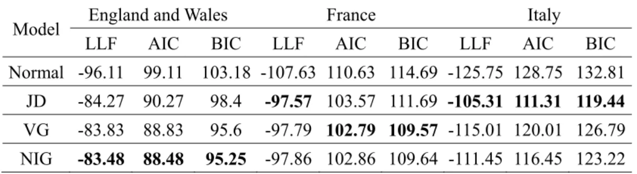
(12) 2009; Haberman and Renshaw, 2009). However, with the Poisson error structure, the intensity at age x and time t is determined by the death rate at age x and time t, which is broadly described by stochastic mortality models. Consequently, instead of using a Poisson model with a deterministic intensity function, an alternative means of fitting the number of deaths is to specify a doubly stochastic Poisson process, or Cox process (Cox, 1955), to capture the stochastic intensity. Biffis et al. (2010) first implement a doubly stochastic setup in the LC model, introducing a class of equivalent probability measures for pricing life insurance liabilities and mortality-indexed securities. Following the double stochastic setup proposed by Biffis et al. (2010), the second. 治政大 for estimating the Cox goal of this article is to provide an iterative fitting algorithm 立 regression model in which mortality rates adhere to the RH model with non-Gaussian. ‧ 國. 學. innovations.. ‧. In Chapter 4, we use three mortality data sets—England and Wales, France, and. sit. y. Nat. Italy—from 1900 to 2008 as the observed data. We first fit the model to the mortality. io. er. rates from 1900 to 1983 using the normal, JD, variance gamma (VG), and NIG distributions, and then we forecast the development of the mortality curve for the. al. n. v i n subsequent 25 years. AccordingCtohthe Jarque-Bera statistical test, the assumption of engchi U normality must be rejected for the logarithm of mortality rates. Finally, according to. the mean absolute percentage errors (MAPEs) of the mortality projections, our empirical results indicate that the RH model with non-Gaussian innovations is the most appropriate choice for modeling long-term mortality data. In addition, as an application for England and Wales, we provide the fair values of longevity swaps and their value at risk (VaR) and conditional tail expectations (CTE). According to the RH model with non-Gaussian innovations, the swap premiums are lower, but the VaR and CTE are higher, which means that using the RH model with non-Gaussian 5 .

(13) innovations can reduce the costs of the longevity risk hedger and avoid the underestimation of loss reserves. In finance field, the past three decades has sparked the development of a large body of theory concerning multivariate probability distributions. Most studies about multivariate asset models are based on Brownian motions due to their simple structure. However, since the work of Mandelbrot and Taylor (1967) and Clark (1973), it has been widely recognized the presence of significant skewness and excess kurtosis in empirical asset return distributions; that is, the returns are non-normally distributed. To allow for both kurtosis and skewness for the multivariate probability distribution. 治政 of assets returns, multivariate Lévy processes are also大 used as a tractable model for 立 asset returns.. ‧ 國. 學. There are essentially two multidimensional models for financial asset pricing:. ‧. one is multivariate normal mixtures based on a common mixing distribution and the. sit. y. Nat. other is multivariate time-changed Brownian motions based on a common time. io. er. change. Barndorff-Nielsen (2001), Cont and Tankov (2004), Luciano and Schoutens (2006) and Eberlein and Madan (2009) provide a multivariate time changed Brownian. n. al. Ch. motion by a common subordinator. As noted in. engchi. iv n Luciano U. and Semeraro (2010),. however, the common subordinator exerts a strict restriction on the joint process, which in turn leads to the lack of independence. Semeraro (2008) and Luciano and Semeraro (2007) propose a similar model with idiosyncratic and systematic subordinators to capture idiosyncratic and systematic jump shocks simultaneously. In this line, Luciano and Semeraro (2010) consider correlated Brownian motions with idiosyncratic and systematic subordinators to increase the range of dependence using correlated Brownian motions. However, as noted in Luciano and Semeraro (2010), this approach is still less flexible in terms of high correlation. 6 .

(14) Since the introduction of the generalized hyperbolic distributions (GH) by Barndorff-Nielsen (1977, 1978), it has widely been used in many applications because it provides a flexible tool for modeling the empirical distribution of financial data exhibiting skewness, leptokurtosis and fat-tails. The GH distribution encompasses many other distributions as special case, which includes the well-known normal inverse Gaussian (NIG) distributions of Barndorff-Nielsen (1995) and the Variance Gamma (VG) distributions of Madan and Seneta (1987, 1990). Multivariate GH (MGH) distributions were introduced and investigated by Barndorff-Nielsen (1978) and Blasild and Jensen (1981) according to a variance–mean mixture of a multivariate. 治政大distributions to fit financial normal distribution. Prause (1999) first uses the MGH 立. market. However, as Schmidt et al. (2006) show, it is computational burdensome to. ‧ 國. 學. estimate the MGH distribution parameters since all parameters must be estimated. ‧. simultaneously. Also, the MGH distributions do not allow independent margins, and. sit. y. Nat. they are not able to model tail-dependence.. io. er. Schmidt et al. (2006) introduced multivariate affine generalized hyperbolic (MAGH) distributions. Because MAGH distributions are defined as an affine. al. n. v i n C hmargins, these distributions transformation of independent GH possess four desirable engchi U. features: easier for estimation and simulation algorithms, the existence of characteristic functions in closed form, better goodness-of-fit that MGH distributions, and the ability to capture a wide range of dependence structure. More recently, Fajardo and Farias (2010) price multidimensional European derivatives by obtaining the density resulting from the convolution of MAGH distributions. Distinct from Schmidt et al. (2006) and Fajardo and Farias (2010) who use the univariate GH distributions with zero location and unit scaling to construct MAGH distributions, we use standard GH margins to construct MAGH distributions. 7 .

(15) The demand on more sophistical multivariate distributions on modeling asset prices poses implies that in many cases, closed form solutions does not exist on the price of the derivative securities. It is numerically even more challenging to price Bermudan/American options. While there exists many numerical methods for pricing Bermudan/American options when there is only one underlying asset price, many of these methods are breakdown when the option depends on more than one asset. An example is the multinomial tree of Këllezi and Webber (2004) and Maller et al. (2006) which is known to be very efficient for pricing Bermudan/American options when there is one underlying asset in Lévy process models. However, if the option depends. 治政 on more than one asset, the multinomial tree becomes大 computational infeasible. For 立 derivative pricing under multivariate Brownian motion, a possible method is the. ‧ 國. 學. stochastic mesh (Monte Carlo mesh; for short MCM) method of Broadie and. ‧. Glasserman (2004) and low discrepancy mesh (LDM) method of Boyle, et al. (2003).. sit. y. Nat. In Boyle et al. (2003), they have shown that the LDM method can be a competitive. io. er. method to price multivariate Bermudan/American options. Their studies, however, have confined to assuming that the returns of the assets are multivariate normally. n. al. distributed.. Ch. engchi. i n U. v. In Chapter 5, we are concerned with an efficient algorithm of pricing multivariate Bermudan options assuming that the underlying asset returns follow MAGH distributions. To the best of our knowledge, there is no other numerical works that have used these distributions to price Bermudan derivatives. Here we demonstrate that LDM method can be extended to price Bermudan options even when the underlying asset returns follow MAGH distributions. In addition, in consistent with the results of Boyle et al. (2003), the LDM estimates are higher bias while the estimates from the Least Square Method (LSM) of Longstaff and Schwartz (2001) are 8 .

(16) low bias. This property also ensures that the true value will lie between these two bounds. The remainder of this thesis is organized as follows. In Chapter 2, we introduce heavy-tailed distributions. We then illustrate the Lee-Carter model with t, JD, VG, NIG, and GHST innovations, as well as provide the dynamics of the mortality indices in Chapter 3. In Chapter 4, we provide a an iterative fitting algorithm to generate the maximum likelihood estimates of the Cox regression model under which the residuals of the RH model, the mortality indices and the cohort effects adhere to heavy-tailed distributions. And we employ the RH model with non-Gaussian innovations to price a. 治政 longevity swap and calculate its VaR and CTE using大 England and Wales mortality 立 data. The final application is in Chapter 5. We present the MAGH distributions as. ‧ 國. 學. well as the estimation algorithm, and we employ the MAGH processes for asset. ‧. returns, providing the multivariate Esscher transform for the MAGH asset model.. sit. y. Nat. However, we demonstrates the convergence of our proposed method by using some. io. er. high dimensional Bermudan options when the underlying assets follow a MAGH distribution. In the end of thesis, we have some conclusions.. n. al. Ch. engchi. 9 . i n U. v.

(17) 立. 政治大. ‧. ‧ 國. 學. n. er. io. sit. y. Nat. al. Ch. engchi. 10 . i n U. v.

(18) Chapter 2 政治大. 立 Distributions Heavy-Tailed ‧. ‧ 國. 學. 2.1 Introductions of Heavy-Tailed Distributions. y. Nat. n. al. Ch. i 1. engchi U. er. io. N. X  a   Z   Yi ,. sit. If a random variable X adheres to a JD distribution, then. v ni. (2-1). where N follows the Poisson distribution with intensity  N ; Z is a standard normal random variable; and each Yi , independent of z and N, is a normal distribution with mean Y and variance  Y2 . Therefore, the probability density function takes the form: . f JD  x a,  , N , Y , Y      x; a  N Y ,  2  NY2 N  i  Prob  N  i  , i 0. .  i 0. Ni e. N. i!.   x; a  iY ,  2  iY2  ,. (2-2). where  ( x;  ,  2 ) is a normal probability density function with mean  and 11 .

(19) variance  2 . The characteristic function of the JD distribution is of the form:. . . JD  a,  , N , Y , Y   exp ia  0.5 2 2  N ei  0.5   1  . . 2 2 Y. Y. (2-3). However, the first two moments of the JD distribution are. E  X   a  N Y ,. (2-4). Var  X    2   N  Y2   Y2  .. (2-5). The moment-generating function is  JD  i a ,  ,  N , Y ,  Y  . The t, VG, NIG, and GHST distributions are the special cases of the generalized. 政治大. hyperbolic (GH) model proposed by Barndorff-Nielsen (1977, 1978) and offer. 立. flexible tools for modeling the empirical distribution of financial data that exhibit. ‧ 國. 學. skewness, leptokurtosis, and fat tails.1 The generalized hyperbolic probability density function, following Prause (1999), is. 2 K    2   2.   x . Ch. engchi. 1  2. .  2 x  .   2   x   2    . i n U. v. 2. y. . e. n. al. K. sit. . er. io.  .    . ‧. Nat. fGH  x  ,  ,  ,  ,   .  2 2    . 1. 2   . .  , (2-6). where K  is the modified Bessel function of the second kind with index  ;  is the scale parameter;  is the shift parameter; and  ,  and  determine the shape of the GH distribution. The parameters must fulfill the following constraints:.   0 ,    if   0 .   0 ,    if   0 .   0 ,    if   0 .. (2-7).                                                         1. In the empirical analyses, we also use the GH distribution to fit the mortality data of our six countries. However, the calibration results of the GH distribution always reduce to those of the GHST distribution, so we focus on this special case instead of the broader GH distribution. 12 .

(20) The characteristic function of the GH distribution is of the form:. . . 2  2 2  2 K        i  i  GH   ,  ,  ,  ,    e  2        i 2  K   2   2  . .. 2. . . (2-8). However, the first two moments of the GH distribution are EX    .  . , . K  1   2   2. .  2   2 K. 2  2. (2-9).     政治   . (2-10)  大 K               立    K        . . 2.  1. 2. . 2. 2. 2. 學. ‧ 國.  K  1   2   2   2 2 2 2      K     Var  X    2  K  2  2 2   2    2 2  2 2  K      . The moment-generating function is GH  i  ,  ,  ,  ,   .. ‧. If we let   0,   0 in Equation (2-6), using K  ( x ) ~  ( )2 1 x   as   0. y. Nat. n.   x  ,  , ,   . fVG.  C. a2   2. l. . x.   0.5. er. io. sit. and x  0 , we can obtain the VG distribution, with the following density function:. K  0.5  x   . he 2n g ch i    0.5. i n U. v. exp    x     . (2-11). Note that when    G  M  2 ,    G  M  2 , and   C , we obtain the VG distribution, which is a special case of the CGMY distribution defined by Carr et al (2002). The characteristic function of the VG distribution is of the form:  2 2 VG   ,  ,  ,    ei  2       i 2 . .   .  . (2-12). However, the first two moments of the VG distribution are. E X    . 2 , 2  2 13 . . (2-13).

(21) Var  X  . 2  2 2  1   . 2  2  2  2 . (2-14). The moment-generating function is VG  i  ,  ,  ,   . The another popular representation of the VG distribution is provided in Appendix A. 0.5  x When   0.5 , realizing that K0.5 ( x)   2 x e and K   ( x )  K  ( x ) ,. we obtain the NIG distribution with the following density function:.   K1    2   x   2      . (2-15) f NIG  x  ,  ,  ,    exp    2   2    x          2   x   2. 政治大 The characteristic function of the NIG distribution is of the form: 立. ‧ 國. .    2. 2. n. Ch.  2.  2   2 . 1.5. y. ,. (2-17). sit. io. al. 2 2. .. engchi U. er. Nat. Var  X  . . ‧. However, the first two moments of the NIG distribution are EX    . . 2   2     i   . (2-16) . 學. NIG   ,  ,  ,    exp  i  . v ni. (2-18). The moment-generating function is  NIG  i  ,  ,  ,   . This distribution is one of the most promising versions of the GH distribution for asset returns, because it possesses several attractive theoretical properties and analytical tractability. It therefore appears frequently in financial applications as an unconditional return distribution (Bølviken and Benth, 2000; Eberlein and Keller, 1995; Lillestøl, 2000; Prause, 1997; Rydberg, 1997) and for stochastic mortality modeling (Giacometti et al., 2009). The another representation of the NIG distribution is provided in Appendix B. If instead we let   v / 2 and    14 . in Equation (2-6), and we realize that.

(22) K  ( x ) ~  (  )2   1 x  as   0 and x  0 . In addition, K  ( x )  K   ( x ) . We can obtain the density of the GH skew Student’s t-distribution (GHST), proposed by Aas and Haff (2006), as follows:. fGHST  x  , v,  ,   .  2 2   x     . v 1 2. v . . v 1 2. e  x . v1 2. (2-19).  2 (v 2)   K v 1   2 . .  2   x   2  ,   0. . The characteristic function of the GHST distribution is of the form:. 治政    i   K 大  2  . 2. 2. 立. GHST   , v,  ,    e. i . . 2.  2  i. 2. . v 1 2. ,   0.. (2-20). 2  (v 2). ‧ 國. 學. However, the first two moments of the GHST distribution are. . y. 2. 2   2    4    2. sit. io. n. al. 2 2 4. (2-21). .. (2-22). er. Nat. Var  X  .  2 ,  2. ‧. EX    . Ch. i n U. v. The moment-generating function of the GHST distribution is undefined.. engchi. The GHST distribution is one of the skew extensions of Student’s t-distribution. Letting   v and   0 in Equation (2-19), we obtain the non-central Student’s. t-distribution with v degrees of freedom, as follows:  v 1 v 1 )   x   2  2 2 . ft -distribution  x v,    1   v  v    v ( )  2. (. (2-23). The characteristic function of the non-central Student’s t-distribution is of the form:. 15 .

(23) t -distribution  v,    e. i . . . v. 2. K 2. . v 2. 2. . v 1 2. ,. (2-24). 2 (v 2). However, the first two moments of the non-central Student’s t-distribution are. E  X   ,   1 , Var  X  .   2. (2-25). ,   2.. (2-26). In order to standardization, we first introduce the three parameters of Student's. t-distribution (Bishop, 2006). We illustrate how to implement the Student's. 政治大. t-distribution in next subsection. The probability density function of three parameters. 立. f t -distribution  x v,  ,   . 學. ‧ 國. of Student's t-distribution is.   v 1 v 1 )    x   2  2 2 . 1   v  v v    ( )  2. (. (2-27). ‧. . n. a. t -distribution  v,  ,l C  ei.  v 2  2  v 2    K      2      , v 1 2 2 (v 2). er. io. sit. y. Nat. where  is called the precision of the Student's t-distribution. The characteristic function of the three parameters of Student’s t-distribution is of the form:. hengchi. i n U. v. (2-28). However, the first two moments of the three parameters of Student’s t-distribution are. E  X   ,   1 , Var  X  .  ,   2.    2 . The moment-generating function of the Student’s t-distribution is undefined.. 16 . (2-29) (2-30).

(24) 2.2 The Standardization Approaches for Heavy-Tailed Distributions In the subsection, we introduce the standardizations of the JD, GH, VG, NIG, GHST and Student's t-distribution . We let. X  a  b  ,. (2-31). where  are standardized random variables (i.e. E     0 and Var     1 , imply. E  X   a and Var  X   b2 ).  can be one of the standardized Lévy Processes. We can choose a finite-activity jump process, the jump-diffusion model of Merton. 政治大. (1976), and an infinite-activity jump process, the GH model.. 立. 學. ‧ 國. From Equation (2-4) and (2-5), if  follows a standardized JD distribution, then N.   N Y  1  N  Y2   Y2   Z   Yi ,. (2-32). i 1. ‧. where N is the Poisson distribution with intensity  N ; Z is a standard normal. Nat. sit. y. random variable; each Yi , independent with Z and N, is a normal distribution with. er. io. 2 mean  Y and variance Y . The  setting satisfies E     0 and Var     1 .. n. al. i n The probability density functionC of  is of the form hengchi U. v. f JD  y  N , Y ,  Y . . . e  N Ni   y -N Y  i Y , 1  N  Y2   Y2   i Y2 , i! i 0 . . where  y  ,  2. . . . (2-33). is the probability density function with mean  and variance.  2 for y. Barndorff-Nielsen (1977, 1978) proposes the generalized hyperbolic (GH) model and the t, VG, NIG and GHST distributions are the special cases of the GH model. From Equation (2-9) and (2-10), if  follows a standardized GH distribution, then 17 .

(25)  2 2    . fGH  y  ,  ,   .  .    . . K. 2 K      2. 2. . e.   y . 1  2. .  2  y  .   2   y   2    .    . 2. 1  2. ,. (2-34). where  and  must satisfy the first two moments:. E ( )   . K  1   0,  2   2 K  . . (2-35). 2 2  2 K  1     2   K   2    K  1       V ( )    1,   K        K     K     . (2-36).   政治大 is the modified Bessel function of the second kind with index λ; 立. where K . ‧ 國. 學.     2   2 ;  is the shift parameter and  is the scale parameter. In accordance with λ, α and β we can describe the shape of the GH distribution. When. ‧.   0 , the shape is symmetric. In addition, these parameters obey the following. y. Nat. er. io. sit. constraints:     0 and   R .. From Equation (2-13) and (2-14), we can obtain  follows a standardized VG. n. al. distribution: fVG  y  ,  .  . 2. Ch. engchi. 2 y .   0.5.   2 . . 2. . . . v. K   0.5  y  .   0.5. 2 2.   2  and   where    2 2   2 2  2. i n U.   .  e . y . ,. (2-37). such that E   t   0 and Var   t   1 .. From Equation (2-17) and (2-18), we also obtain that  t follows a standardized NIG distribution:. 18 .

(26)   K1    2   y   2      , (2-38) f NIG  y  ,    exp    2   2    y          2   y   2. where. . .  . and. 2 2. 2. 2. 1.5. such. 2. that. E    0. and. Var     1 . From Equation (2-21) and (2-22), we have standardized GHST distribution, as follows:. fGHST  y  , v  . .  2治 2 政 e    y   大  v 1 2. . . v 1 2.   y  . . v1 2. (2-39).  2 (v 2)   K v 1   2 . 學 .  2   y   2  ,   0. . ‧. ‧ 國. 立. v. where  and  must satisfy the first two moments:. y. sit. io. a 2     1i.v Var  l   Ch 2   4  U2 n engchi n. 2. 4. 2. (2-40). er. Nat.  2 E      0,  2 2. (2-41). For standardized Student's t-distribution, we employ the three parameters of Student's t-distribution to transfer. From Equation (2-29) and (2-30), we obtain that  t follows a standardized Student's t-distribution: f t -distribution  y v  . where   0,   1 and  .  v 1 v 1 )    y   2  2 2 , 1   v  v v    ( )  2. (.  2 ,   2 such that E     0 and Var     1 . . 19 . (2-42).

(27) 2.3 Estimation Scheme with Standardization To estimate parameters of these models, we use the maximum likelihood method. Let a time series.  X t t 1 , and they are independent and identically distributed (i.i.d.), n. as follows:. . i .i.d .. . X t  f X a, b 2  ,. (2-43). where X is a random variable with parameters  ; a represents the mean of X and b represents the standard derivation of X. Or equivalently, we have. 立. 政治大. X t  a  b t ,. (2-44). ‧ 國. 學. where  t are standardized random variables (i.e. E   t   0 and Var   t   1 , imply E  Rt   a and Var  Rt   b2 ) and independent and identically distributed. ‧. (i.i.d.). The log-likelihood function with respect to  is. (2-45). er. io. al. . y. . t 1. sit. Nat. n. LLF   ln f X  X t . v. n. where  d ; d is the number of the unknown parameters. From Equation (2-44), we have. Ch. engchi. t . i n U. Xt  a . b. (2-46). Using transformation of random variable, if the probability density function of random variable U is given by fU ( x ) and h is a monotonic function and we know the probability density function of V  h U  is fV  v   fU  h. 1. v  . 20 . d  h 1  v   dv. (2-47).

(28) where h1 denotes the inverse function. So equivalently, we let h 1  X t  . Xt  a b. and rewrite Equation (2-47) as follows:.  X a 1 f X  x   f  t   b  b. (2-48). Considering Equation (2-48), substituting into Equation (2-45) we obtain n     X  a  LLF   ln  f   t    ln  b   b  t 1     . (2-49). Originally we estimate parameters with respect to random variable Rt , using the. 政治大. method of standardization, we change to random variable  t when estimating. It is. 立. an advantage for reducing the number of estimated parameters. For example, assume. ‧ 國. 學. the logarithm returns follow GH distribution, we need estimate five parameters  ,.  ,  ,  ,  if we do not use standardization approach. But we just estimate three. ‧. parameters  ,  ,  when we employ standardization approach.. n. er. io. sit. y. Nat. al. Ch. engchi. 21 . i n U. v.

(29) 立. 政治大. ‧. ‧ 國. 學. n. er. io. sit. y. Nat. al. Ch. engchi. 22 . i n U. v.

(30) Chapter 3 政治大. ‧. ‧ 國. 學. 立 Comparison of the A Quantitative Lee-Carter Model under Different Types of Non-Gaussian Innovations n. er. io. sit. y. Nat. al. i n U. Ch. v. n g c h i Innovations 3.1 The Lee-Carter Model witheHeavy-Tailed In this Chapter, we first review the classical Lee-Carter model, under which the mortality index follows an ARIMA model with normal innovations. Using the mortality data of six countries, we find that all the residuals of the Lee-Carter model and the mortality indices exhibit non-zero skewness and excess kurtosis. Therefore, we use the Lee-Carter model with five non-Gaussian distributions—t, JD, VG, NIG, and GHST—to model both the residuals and the dynamics of the mortality indices. The Lee-Carter Model. We analyze the changes in mortality as a function of both age x and time t. The 23 .

(31) mortality forecast relies on the classical Lee-Carter model, namely, ln  m x ,t    x   x k t  e x ,t ,. (3-1). where mx ,t is the central death rate for age x in calendar year t, defined as the span from time t to time t 1 . This structure is designed to capture age–period effects;  x describes the average pattern of mortality for the age group;  x represents the. age-specific patterns of mortality change, indicating the sensitivity of the logarithm of the force of mortality at age x to variations in the time index k t ; k t explains the time trend of the general mortality level; and ex ,t represents the deviation of the. 治政 model from the observed log-central death rates,大 which should be 立 distribution with zero mean and a relatively small variance (Lee, 2000).. a normal. ‧ 國. 學. We use approximation to fit the three parameters. According to two constraint. k t. t.  0 and. . x.  1 , ˆ x is simply the average value over time of. ‧. conditions,. x. Nat.  .  . io. sit. y. ln  m x ,t  , and kˆt is the sum over various ages of ln mx,t ˆ x . Using ln mx,t ˆ x. n. al. using a simple regression. er. as the dependent variable and kˆt as the explanatory variable, we can obtain ˆ x by. v i n C h without an intercept model e n g c h i U parameter.. Finally, we. re-estimate the kˆt by iteration, using actual number of deaths, population, ˆ x , and. ˆ x , such that the actual number of deaths is close to the estimated number of deaths, and the adjusted kˆt is denoted as kˆt* . To forecast future mortality dynamics, Lee and Carter (1992) assume that  x and  x remain constant over time and therefore forecast the dynamics of adjusting the mortality index kt* using an ARIMA(0,1,0) model, as follows:. kt*  kt*1     t , 24 . (3-2).

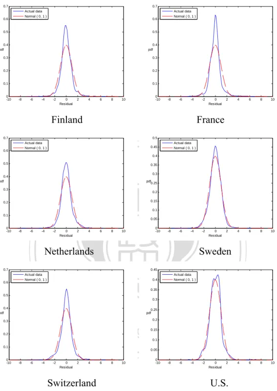
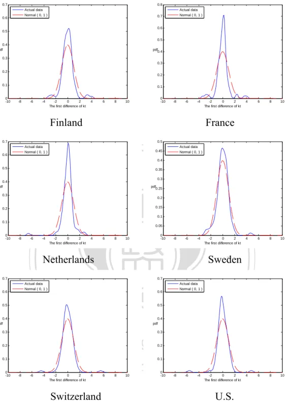
(32) where  is a drift term, and  t is a sequence of independent and identically Gaussian random variables with mean 0 and variance  2 . Normality Tests for the Residuals and Mortality Indices. In this subsection, we apply the JB (Jarque and Bera, 1980) test to determine empirically the normality of the mortality data of six countries (Finland, France, Netherlands, Sweden, Switzerland, U.S.) from 1900 to 2007. The mortality data for the first five countries come from the Human Mortality Database (HMD) website,2 whereas the U.S. data come from the National Center Health Statistics (NCHS). 政治大 First, we examine the normality test for the residuals in Equation (3-1). Figure 立. website.3. ‧ 國. 學. 3-1 depicts the probability density function of the standardized residuals. Clearly, the empirical residuals peak around the mean and fatter tails; that is, the residuals are. ‧. non-normally distributed. Second, Figure 3-2 reveals the patterns of mortality indices,. sit. y. Nat. offering evidence of mortality improvements. We also find a lot of jump points. Chen. al. er. io. and Cox (2009) attribute jump points in the U.S. mortality rate to influenza epidemics. v. n. and argue against the naïve belief that a pandemic is a one-time event that cannot. Ch. engchi. i n U. happen again. We thus cannot just ignore such extreme events. In addition, as we show in Figure 3-3, the probability density functions of the first differences in the mortality indices exhibit higher central peaks and larger tails than does a normal distribution. Therefore, we can fit the mortality indices to the non-Gaussian distributions..                                                         2. http://www.mortality.org/. http://www.cdc.gov/nchs/nvss/mortality_tables.htm. Death rate files: HIST290 and GMWK290R. Death files: HIST290A and GMWK23F. 25 3.

(33) 0.7. 0.7 Actual data Normal ( 0, 1 ). 0.6. 0.5. 0.5. 0.4 pdf. 0.4 pdf. 0.3. 0.3. 0.2. 0.2. 0.1. 0.1. 0 -10. -8. -6. -4. Actual data Normal ( 0, 1 ). 0.6. -2. 0 Residual. 2. 4. 6. 8. 0 -10. 10. -8. -6. -4. Finland. -2. 0 Residual. 2. 4. 6. 8. 10. 2. 4. 6. 8. 10. 4. 6. 8. 10. France. 0.7. 0.5 Actual data Normal ( 0, 1 ). 0.6. Actual data Normal ( 0, 1 ). 0.45 0.4. 政治大. 0.5. 0.35. 0.3. 0.4 pdf. 立. 0.3. pdf 0.25. 0.2 0.15. -6. -4. -2. 0 Residual. 2. 4. 6. 8. 0 -10. 10. -8. -6. -4. 0.45. io. 0.5. 0.35. al. 0.3. n. 0.4 pdf. Actual data Normal ( 0, 1 ). 0.4. 0.3. er. 0.6. Sweden. Nat. Actual data Normal ( 0, 1 ). 0 Residual. ‧. Netherlands. 0.7. -2. y. -8. 0.1 0.05. Ch. 0.2. sit. 0 -10. 學. 0.1. ‧ 國. 0.2. 0.25 pdf 0.2. engchi 0.15. i n U. v. 0.1. 0.1. 0 -10. 0.05. -8. -6. -4. -2. 0 Residual. 2. 4. 6. 8. 0 -10. 10. Switzerland. -8. -6. -4. -2. 0 Residual. 2. U.S.. Figure 3-1. The Probability Density Functions of Standardized Residuals. 26 .

(34) 20. 20. 15. 15. 10. 10. 5 5 0 kt. kt. 0. -5 -5. -10. -10. -15 -20. -15. -25. -20 -25. -30 1900 1910. 1920 1930 1940. 1950 1960 1970 year. 1980 1990 2000. 1900 1910. 1920 1930 1940. Finland. 1950 1960 1970 year. 1980 1990 2000. France 20 15. 15. 10. 政治大. 10. 5. 5. 0. kt. 立. 0 -5. kt. -5. -10 -15. 1900 1910. 1920 1930 1940. 學. -15. ‧ 國. -10. -20 -25. 1950 1960 1970 year. 1980 1990 2000. 1900 1910. 1920 1930 1940. 0 -5. y. sit. 8 6 4. al. n. 5. 10. er. io. 10. kt. Sweden. Nat. 15. 1980 1990 2000. ‧. Netherlands. 20. 1950 1960 1970 year. 2. Ch. -10. kt. 0. engchi -2 -4. i n U. v. -6. -15. -8 -20 -10 1900 1910. 1920 1930 1940. 1950 1960 1970 year. 1980 1990 2000. 1900 1910. Switzerland. 1920 1930 1940. 1950 1960 1970 year. U.S.. Figure 3-2. The Pattern of Mortality Indices. 27 . 1980 1990 2000.

(35) 0.7. 0.8 Actual data Normal ( 0, 1 ). 0.6. Actual data Normal ( 0, 1 ). 0.7 0.6. 0.5. 0.5 0.4 pdf. pdf 0.4. 0.3 0.3 0.2. 0.2. 0.1. 0 -10. 0.1. -8. -6. -4. -2 0 2 The first difference of kt. 4. 6. 8. 0 -10. 10. -8. -6. -4. Finland. -2 0 2 The first difference of kt. 4. 6. 8. 10. 4. 6. 8. 10. 4. 6. 8. 10. France. 0.7. 0.5 Actual data Normal ( 0, 1 ). 0.6. Actual data Normal ( 0, 1 ). 0.45 0.4. 政治大. 0.5. 0.35. 0.3. 0.4 pdf. 立. 0.3. pdf 0.25. 0.2 0.15. -6. -4. -2 0 2 The first difference of kt. 4. 6. 8. 0 -10. 10. -8. -6. -4. ‧. Netherlands 0.6. io. 0.5. 0.7. 0.5. al. n. 0.4 pdf 0.3. Ch. 0.2. 0.4 pdf. engchi 0.3. i n U. v. 0.2. 0.1. 0 -10. Actual data Normal ( 0, 1 ). 0.6. er. Actual data Normal ( 0, 1 ). Sweden. Nat. 0.7. -2 0 2 The first difference of kt. y. -8. 0.1 0.05. sit. 0 -10. 學. 0.1. ‧ 國. 0.2. 0.1. -8. -6. -4. -2 0 2 The first difference of kt. 4. 6. 8. 0 -10. 10. Switzerland. -8. -6. -4. -2 0 2 The first difference of kt. U.S.. Figure 3-3. The Probability Density Functions of the First Difference in Mortality Indices. 28 .

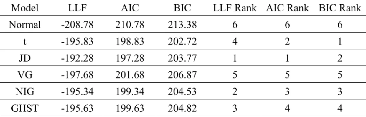
(36) To examine the assumption of normality of mortality rates in the Lee-Carter model, we also use the JB test statistic, a goodness-of-fit measure of the departure from normality:  s 2  k  3 2  JB  n   , 24   6. (3-3). where n is the sample size, s is sample skewness, and k is sample kurtosis. Table 3-1 provides the results of the JB test, together with the skewness and excess kurtosis values, for the residual of the Lee-Carter model and the first difference of the. 政治大 different from zero, and the excess kurtosis is large. The JB statistics also are 立 six countries’ mortality indices from 1900 to 1999. The skewness is significantly. significantly large, which means we must reject the assumption of normality. In turn,. ‧ 國. 學. we use the heavy-tailed distributions—t, JD, VG, NIG, and GHST—to model the. ‧. non-Gaussian property of the error terms in Equations (3-1) and (3-2).. sit. y. Nat. Table 3-1. Skewness, Excess Kurtosis and the Jarque-Bera Test. Country. 0.394. Skewness. (0.053 ). Excess Kurtosis JB Test. al. n. Finland. France. Netherlands. er. io. Panel A: the Residuals of the Lee-Carter Model Sweden. v i 0.950 -0.298 -0.100 n Ch g c h) i U (0.053e ) n (0.053 (0.053 ). Switzerland. U.S.. 0.273. 0.444. (0.053 ). (0.074 ). 6.813. 7.168. 6.058. 3.071. 4.925. 4.018. (0.107 ). (0.107 ). (0.107 ). (0.107 ). (0.107 ). (0.148 ). 4116. 4811. 3242. 829. 2148. 776. [< 0.001]. [< 0.001] [< 0.001] [< 0.001] [< 0.001] [< 0.001]. The table presents the skewness and excess kurtosis of the standardized residuals of the Lee-Carter model. Standard errors of the skewness and excess kurtosis given in the parentheses are calculated as. 6 n and. 24 n , respectively. n denotes the number of observations. The p-values of. Jarque-Bera (JB) test are given in bracket.. 29 .

(37) Panel B: the First Difference in Mortality Indices Country Skewness Excess Kurtosis JB Test. Finland. France. Netherlands. Sweden. Switzerland. U.S.. 0.665. 0.441. -2.525. 0.470. 0.827. -0.661. (0.246 ). (0.246 ). (0.246 ). (0.246 ). (0.246 ). (0.246 ). 4.439. 5.339. 18.396. 4.601. 11.446. 13.476. (0.492 ). (0.492 ). (0.492 ). (0.492 ). (0.492 ). (0.492 ). 89. 121. 1501. 91. 552. 756. [< 0.001]. [< 0.001] [< 0.001] [< 0.001] [< 0.001] [< 0.001]. The table presents the skewness and excess kurtosis of the first difference in mortality indices. Standard errors of the skewness and excess kurtosis given in the parentheses are calculated as and. 6 n. 24 n , respectively. n denotes the number of observations. The p-values of Jarque-Bera (JB). test are given in bracket.. 治政大 The Lee-Carter Model with Non-Gaussian Distributions 立. Because the residuals of the Lee-Carter model and the mortality indices are. ‧ 國. 學. non-normally distributed, we model the error term, ex ,t and  t , using the five. ‧. heavy-tailed distributions: t, JD, VG, NIG, and GHST. These distributions are refered. sit. y. Nat. to Chapter 2.. n. al. er. io. For mortality data at age x  1,..., g and time period t  1,..., T , the calibrated. v. parameters of the Lee-Carter model can be obtained by maximizing the sample log-likelihood function (LLF),. Ch. g. engchi T. . i n U. . LLF   ln f  ext   , x 1 t 1. (3-4). k. with respect to  , which satisfies two constraint conditions,. t.  0 and. t. . x.  1 .4 As suggested by Lee and Carter (1992), we re-estimate the k t factors by. x. iteration, given the values of  x and  x we obtained in the maximum likelihood                                                         4 Let a    in the JD model and     K  1   2   2. . . .  2   2 K   2   2. the special cases of the GH model. Thus, we ensure that the mean of error terms equals 0. 30 . . in.

(38) estimation, such that the implied number of deaths equals the actual number of deaths, or. Dt   N x , t exp  x   x kt , t  1,..., T ,. (3-5). x. where D t is the total number of deaths in year t , and N x ,t is the total population of age group x at time t . Using the re-estimated mortality indices, we can calculate the parameters of Equation (3-2) by maximizing the log-likelihood function, as follows: T.   .  ln  f 治政大. 立. (3-6). t. t 1. ‧ 國. 學. 3.2 Empirical Analysis. In this section, we illustrate the mortality data and investigate the goodness-of-fit. ‧. distributions for the residuals of the Lee-Carter model and the first difference of. y. Nat. sit. mortality indices. Using the mortality data from 1900 to 1999, we first fit the residuals. n. al. er. io. of the Lee-Carter model with our six distributions: normal, t, JD, VG, NIG, and. i n U. v. GHST. We then fit the first difference of k t from the best goodness-of-fit model,. Ch. engchi. according to the Bayesian information criterion (BIC), to the same six distributions and project the subsequent eight-year mortality rates. Model Comparison. For the sake of comparison, we use the log-likelihood function (LLF), Akaike information criterion (AIC; Akaike, 1974), BIC (Schwarz, 1978), KS test (Kolmogorov,. 1933),. Anderson-Darling. (AD). test. (Stephens,. 1974),. and. Cramér-von-Mises (CvM) test (Anderson, 1962) as goodness-of-fit measures. The AIC is defined as 31 .

(39) AIC   LLF  NPS ,. (3-7). where NPS is the effective number of parameters being estimated. The BIC is defined as. BIC  LLF  0.5  NPS  log  NOS  ,. (3-8). where NOS is the number of observations. For these criteria, a higher value of LLF and a smaller value of AIC and BIC indicate a better goodness of fit for the mortality model. For the KS test, the null hypothesis is H 0 : G  x   F  x;  for all sample data x. 政治大. and the parameters  of the distribution, where G  x  represents the empirical. 立. distribution function of the sample mortality index, and F  x;  is the hypothesized. ‧ 國. 學. cumulative density distribution (CDF). The test statistic is defined as. ‧. KS  sup F  x;    G  x  .  x. Nat. y. (3-9). n. al. er. io. model.. sit. Thus a higher p-value in the KS test means a better goodness of fit for the mortality. i n U. v. The AD test is a modification of the KS test, which also determines whether a. Ch. engchi. sample of data come from a specific distribution. However, unlike the KS test, the AD test focuses on the weight of the tail. Its null hypothesis is that the data follow a specific distribution. The AD test statistic is defined as. where NOS. S i 1.  2i  1 ln F NOS . AD2   NOS  S ,. (3-10).  yi ;   ln 1  F  yNOS 1i ;   ;. (3-11). F is a cumulative distribution function of the specified distribution; and y i are the observed values in increasing order. A lower value of the test statistic indicates a 32 .

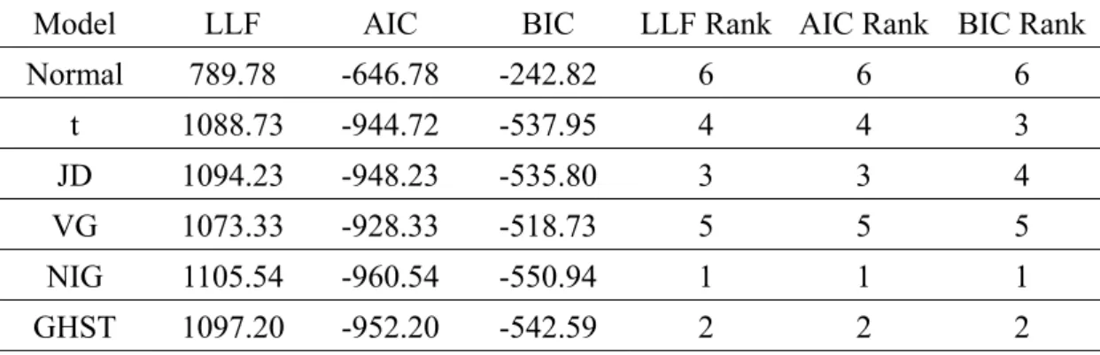
(40) higher possibility that the mortality data come from the distribution F. The CvM test, an alternative to the KS test, is a criterion used to judge the goodness of fit of a probability distribution, compared with a given empirical distribution function. The test statistic CvM is defined as 2. NOS 1  2i  1  CvM    F ( yi ;  )  . 12 NOS i 1  2 NOS . (3-12). A lower value of this test statistic indicates a higher possibility that the mortality data come from the distribution F. Each test offers some benefits. That is, the KS test is known for the independence of its critical values from the tested distribution.. 政治大. Compared with the KS test, the main advantage of the AD test is that it assigns more. 立. weight to the tails of the distribution. Similarly, the CvM test incorporates information. ‧ 國. 學. about the total sample and is insensitive to a slight dislocation of the empirical CDF.. ‧. However, a major disadvantage of the CvM and AD tests is that the critical values depend on the analyzed distribution.5. y. Nat. io. sit. In-Sample Goodness of Fit. n. al. er. Using mortality data from Finland, France, the Netherlands, Sweden,. Ch. i n U. v. Switzerland, and the United States, Table 3-2 provides the LLF, AIC, and BIC results,. engchi. together with their corresponding ranks. All three criteria indicate that the normal distribution is the worst model for all our mortality data. However, the JD model is the best model for the French mortality data; the NIG model is the best for the mortality data of Finland, the Netherlands, and Switzerland; and the VG model is the best option for Sweden. For the U.S. mortality data, the JD model offers the best fit according to the LLF and AIC values, but the t model is the best according to the BIC. In Table 3-3 we report the results for the KS, AD, and CvM tests, together with                                                         5. We obtain the critical values through a Monte Carlo simulation with the estimated parameters (see Chernobai et al., 2007, p. 219). 33 .

(41) their critical values for all six countries. For each country, the three test statistics are greater than the 5% critical value, so the empirical distribution of the residuals does not follow a normal distribution. For the Netherlands and Sweden, no test results reject the null hypothesis that the residuals come from non-Gaussian distributions. In addition, except for the U.S. mortality data, the results of the three tests support the null hypothesis that the residuals come from the best BIC models. For the U.S. mortality data though, the KS statistic rejects the t model, which is the best model according to the BIC, at a 1% significance level. Thus the difference between the theoretical and empirical CDF appears significant. However, if we ignore the. 治政大 goodness of fit for the U.S. dislocation of the empirical CDF, the t model offers better 立. residuals, from the standpoint of the AD and CvM tests. Because the AD and CvM. ‧ 國. 學. test results do not reject the claim that the error terms in Equation (3-1) come from the. ‧. best models, according to the BIC, we use the mortality indices obtained from the best. y. sit. io. n. al. er. . Nat. BIC model to investigate the pattern of innovations in Equation (3-2).. Ch. engchi. 34 . i n U. v.

(42) Table 3-2. Goodness-of-fit Measures for the Residuals of the Lee-Carter Model. Panel A: the Finland Mortality Data Model. LLF. AIC. BIC. LLF Rank AIC Rank BIC Rank. Normal. 789.78. -646.78. -242.82. 6. 6. 6. t. 1088.73. -944.72. -537.95. 4. 4. 3. JD. 1094.23. -948.23. -535.80. 3. 3. 4. VG. 1073.33. -928.33. -518.73. 5. 5. 5. NIG. 1105.54. -960.54. -550.94. 1. 1. 1. GHST. 1097.20. -952.20. -542.59. 2. 2. 2. Panel B: the France Mortality Data Model. LLF. AIC. BIC. LLF Rank AIC Rank BIC Rank. Normal. 826.85. t. 1279.79. JD. 1344.31. VG. 1277.39. -1132.39. -722.78. 5. NIG. 1336.77. -1191.77. -782.17. 2. GHST. 1296.69. -1151.69. -742.08. 3. 學. BIC. Normal. 1878.08. -1735.08. -1331.13. t. 2094.57. JD. 2103.27. Ch -1957.27. VG. 2102.66. -1957.66. NIG. 2118.45. GHST. 2095.81. n. al. -1950.57. 4. 4. 1. 1. 5. 5. 2. 2. 3. 3. y. LLF Rank AIC Rank BIC Rank. -1543.79. e-1544.84 ngchi. 6. i n U2 5. v. 6. 6. 5. 4. 3. 3. -1548.06. 3. 2. 2. -1973.45. -1563.85. 1. 1. 1. -1950.81. -1541.21. 4. 4. 5. 35 . 6. sit. AIC. io. LLF. er. Nat. Panel C. the Netherlands Mortality Data. Model. 6. ‧. ‧ 國. 治 6 -683.85 政-279.90 大 -1135.79 -729.02 4 立 -1198.31 -785.88 1.

(43) Panel D: the Sweden Mortality Data Model. LLF. AIC. BIC. LLF Rank AIC Rank BIC Rank. Normal. 1856.17. -1713.17. -1309.21. 6. 6. 6. t. 1918.32. -1774.32. -1367.54. 5. 5. 2. JD. 1920.62. -1774.64. -1362.22. 2. 4. 5. VG. 1922.51. -1777.51. -1367.91. 1. 1. 1. NIG. 1919.66. -1774.66. -1365.06. 4. 3. 4. GHST. 1920.00. -1775.00. -1365.40. 3. 2. 3. Panel E: the Switzerland Mortality Data Model. LLF. AIC. BIC. Normal. 1612.69. -1469.69. -1065.74. t. 1806.21. JD. 1815.79. VG. 6. 6. 6. 4. 4. 3. 3. 1826.48. -1255.43 治 5 政大 -1669.79 -1257.36 3 立 -1681.48 -1271.88 2. 2. 2. NIG. 1843.55. -1698.55. -1288.95. 1. 1. 1. GHST. 1806.74. -1661.74. -1252.14. 4. 5. 5. 學. ‧. ‧ 國. -1662.21. Panel F: the U.S. Mortality Data. LLF Rank AIC Rank BIC Rank. Normal. 1199.95. -1074.95. -756.82. 6. t. 1273.77. -1147.77. -827.09. 4. JD. 1277.47. -1149.47. -823.71. 1. VG. 1271.16. al. NIG GHST. y. BIC. io. 6. 6. 3. 1. sit. AIC. er. LLF. Nat. Model. 4. 5. 5. 2. 2. 1274.19. -1147.19. 4. 3. n. 1. 1274.83. v i -1144.16 -820.94 5 n Ch n g c h i U2 -1147.83 e-824.61 -823.97. . 36 . LLF Rank AIC Rank BIC Rank. 3.

(44) Table 3-3. Goodness-of-fit Tests for the Residuals of the Lee-Carter Model. Panel A: the Finland Mortality Data KS Model. Statistic. AD. Critical Value 5%. 1%. Statistic. CvM. Critical Value 5%. Statistic. 1%. Critical Value 5%. 1%. Normal 0.061** 0.029 0.035 21.681** 2.443 3.914 3.365** 0.458 0.746 t. 0.031*. 0.029 0.035 2.624*. 2.486 3.868 0.423. 0.463 0.737. JD. 0.024. 0.029 0.035 1.769. 2.491 3.799 0.252. 0.452 0.716. VG. 0.022. 0.029 0.035 1.352. 2.473 3.909 0.190. 0.466 0.747. NIG. 0.016. 0.030 0.035 1.028. 2.516 3.906 0.104. 0.464 0.753. GHST 0.024. 0.029 0.036 1.590. 2.494 4.098 0.188. 0.457 0.786. Note: * and ** denote significance at the 5% and 1% level, respectively.. 政治大 Panel B: the France Mortality Data 立 AD. KS. Critical Value. ‧ 國. Statistic. 5%. 1%. Statistic. Critical Value 5%. 1%. 學. Model. CvM Statistic. Critical Value 5%. 1%. 2.516 3.829 0.970** 0.463 0.724. JD. 0.021. 2.465 3.780 0.176. 0.456 0.716. VG. 0.040** 0.029 0.036 4.513**. 2.467 3.852 0.462*. 0.459 0.727. NIG. 0.026. 2.511 3.951 0.275. 0.461 0.754. 2.511 4.026 0.425. 0.456 0.772. io. 0.029 0.035 2.420. sit. Nat. GHST 0.031*. 0.029 0.035 1.329. y. 0.041** 0.029 0.035 7.765**. er. t. ‧. Normal 0.094** 0.029 0.035 35.657** 2.443 3.914 5.671** 0.458 0.746. al. 0.029 0.035 4.020*. n. v i Note: * and ** denote significance at the 5% and 1% level, respectively. n Ch engchi U. Panel C: the Netherlands Mortality Data KS Model. Statistic. AD. Critical Value 5%. 1%. Statistic. CvM. Critical Value 5%. 1%. Statistic. Critical Value 5%. 1%. Normal 0.062** 0.029 0.035 18.743** 2.443 3.914 3.118** 0.458 0.746 t. 0.023. 0.029 0.035 1.705. 2.533 3.807 0.210. 0.466 0.726. JD. 0.018. 0.029 0.035 0.858. 2.473 3.762 0.130. 0.458 0.710. VG. 0.024. 0.029 0.035 2.336. 2.448 3.742 0.272. 0.454 0.727. NIG. 0.013. 0.030 0.035 0.335. 2.547 3.899 0.038. 0.470 0.741. GHST 0.019. 0.029 0.035 1.692. 2.483 3.897 0.194. 0.460 0.758. Note: * and ** denote significance at the 5% and 1% level, respectively.. 37 .

(45) Panel D: the Sweden Mortality Data KS Model. Statistic. Normal 0.031*. AD. Critical Value 5%. 1%. 0.029. 0.035. Statistic. CvM. Critical Value 5%. 1%. 3.721*. 2.443. 3.914. Statistic. Critical Value 5%. 1%. 0.590*. 0.458. 0.746. t. 0.015. 0.029. 0.035. 0.571. 2.488. 3.881. 0.084. 0.466. 0.751. JD. 0.014. 0.029. 0.035. 0.429. 2.472. 3.857. 0.060. 0.452. 0.736. VG. 0.024. 0.029. 0.035. 1.805. 2.477. 3.909. 0.282. 0.466. 0.747. NIG. 0.014. 0.029. 0.035. 0.379. 2.495. 3.893. 0.047. 0.461. 0.740. GHST 0.013. 0.029. 0.035. 0.370. 2.488. 3.879. 0.043. 0.468. 0.732. Note: * and ** denote significance at the 5% and 1% level, respectively.. 政治 AD 大. Panel E: the Switzerland Mortality Data KS Statistic. 立. Critical Value 1%. Statistic. Critical Value. 5%. Statistic. 1%. 學. 5%. ‧ 國. Model. CvM Critical Value 5%. 1%. 0.027. VG. 0.016. NIG. 0.017. GHST 0.025. 0.460 0.742. 0.029 0.035 2.621*. 2.483 3.714 0.421. 0.454 0.719. 0.029 0.035 0.865. 2.456 3.805 0.108. 0.454 0.730. 0.030 0.036 0.699. 2.579 3.978 0.081. 0.473 0.756. 0.029 0.035 2.677*. 2.514 3.885 0.323. 0.464 0.746. io. 2.470 3.948 0.327. y. JD. 0.029 0.035 2.720*. ‧. 0.025. Nat. t. sit. Normal 0.058** 0.029 0.035 17.921** 2.443 3.914 3.033** 0.458 0.746. er. Note: * and ** denote significance at the 5% and 1% level, respectively.. n. al. KS Model. Statistic. i n C Panel F:hthe eU.S. n gMortality cADh i UData. Critical Value 5%. Normal 0.050** 0.039. 1%. Statistic. v. Critical Value 5%. 1%. Statistic. Critical Value 5%. 1%. 0.046. 7.501** 2.491. 3.902. 1.229** 0.464. 0.748. t. 0.047** 0.039. 0.047. 1.711. 2.551. 4.045. 0.296. 0.473. 0.763. JD. 0.047** 0.039. 0.047. 1.346. 2.459. 3.933. 0.234. 0.461. 0.757. VG. 0.038. 0.039. 0.046. 2.291. 2.488. 3.880. 0.361. 0.460. 0.745. NIG. 0.038. 0.039. 0.046. 1.430. 2.479. 4.001. 0.246. 0.455. 0.756. 0.039. 0.046. 1.523. 2.541. 3.868. 0.249. 0.474. 0.744. GHST 0.039*. Note: * and ** denote significance at the 5% and 1% level, respectively.. 38 . CvM.

(46) Table 3-4 contains the results for the LLF, AIC, and BIC and their corresponding ranks in terms of the normal, t, JD, VG, NIG, and GHST distributions for the first difference of mortality indices. The Gaussian model is the worst, according to the LLF, AIC, and BIC. The LLF criterion also indicates that the best goodness-of-fit derives from the NIG model for the Netherlands but from the JD model for the five other countries. Because it introduces a penalty term for the effective number of parameters, the best in-sample goodness of fit changes for the t distribution, except for France and the Netherlands. According to the BIC, the NIG model again is the best fit for the Netherlands, the JD model is the best for France, and the t model is the. 治政大 States. Table 3-5 lists the best one for Finland, Sweden, Switzerland, and the United 立. results for the KS, AD, and CvM tests, together with their critical values, pertaining to. ‧ 國. 學. the error terms of the mortality indices. The results reject the notion that the error. ‧. terms of the mortality indices for France, the Netherlands, and the United States come. y. come. from. non-Gaussian. io. sit. indices. distributions.. er. mortality. Nat. from a normal distribution. All three test results confirm that the error terms of the Therefore,. the. goodness-of-fit tests consistently indicate that non-Gaussian distributions provide. al. n. v i n better in-sample goodness of fitC forhthe error terms of U e n g c h i the mortality indices. . 39 .

(47) Table 3-4. Goodness-of-fit Tests for the First Difference in Mortality Indices. Panel A: the Finland Mortality Index Model. LLF. AIC. BIC. LLF Rank AIC Rank BIC Rank. Normal. -208.78. 210.78. 213.38. 6. 6. 6. t. -195.83. 198.83. 202.72. 4. 2. 1. JD. -192.28. 197.28. 203.77. 1. 1. 2. VG. -197.68. 201.68. 206.87. 5. 5. 5. NIG. -195.34. 199.34. 204.53. 2. 3. 3. GHST. -195.63. 199.63. 204.82. 3. 4. 4. Panel B: the France Mortality Index Model. LLF. AIC. BIC. LLF Rank AIC Rank BIC Rank. Normal. -222.77. t. -204.48. JD. -195.99. VG. -204.51. 208.51. 213.70. 5. NIG. -198.66. 202.66. 207.85. 2. GHST. -202.81. 206.81. 212.01. 3. 學. 6. 6. 4. 3. 1. 1. 5. 5. 2. 2. 3. 4. ‧. ‧ 國. 治 6 224.77 政227.36 大 207.48 211.38 4 立 200.99 207.48 1. AIC. BIC. Normal. -209.29. 211.29. 213.88. t. -184.02. JD. -181.28. a187.02 l C 186.28 h. VG. -181.98. 185.98. NIG. -179.93. GHST. -181.40. n. 190.91. e 192.77 ngchi. 6. i n U2 5. v. 6. 6. 5. 3. 4. 5. 191.17. 4. 3. 4. 183.93. 189.12. 1. 1. 1. 185.40. 190.59. 3. 2. 2. 40 . LLF Rank AIC Rank BIC Rank. er. LLF. io. Model. sit. y. Nat. Panel C: the Netherlands Mortality Index.

(48) Panel D: the Sweden Mortality Index Model. LLF. AIC. BIC. LLF Rank AIC Rank BIC Rank. Normal. -183.24. 185.24. 187.84. 6. 6. 6. t. -175.64. 178.64. 182.53. 3. 1. 1. JD. -174.79. 179.79. 186.28. 1. 4. 5. VG. -176.59. 180.59. 185.78. 5. 5. 4. NIG. -175.65. 179.65. 184.84. 4. 3. 3. GHST. -175.49. 179.49. 184.68. 2. 2. 2. Panel E: the Switzerland Mortality Index Model. LLF. AIC. BIC. Normal. -168.78. 170.78. 173.37. t. -150.54. JD. -147.09. VG. -153.58. 157.43 治 3 政大 152.09 158.58 1 立 157.58 162.77 5. NIG. -151.70. 155.70. 160.89. 4. GHST. -150.37. 154.37. 159.56. 2. Normal. -92.74. 94.74. 97.34. 6. t. -69.39. 72.39. 76.28. 3. JD. -65.90. 77.38. 1. VG. -70.89. NIG. -70.73. GHST. -69.35. io. n. a70.90 l C 74.89 h 74.73. 73.35. 41 . 1. 1. 2. 5. 5. 4. 4. 3. 3. LLF Rank AIC Rank BIC Rank. iv 80.08 5n e n79.92 g c h i U4 78.54. 2. y. BIC. 6. 2. 6. 6. 2. 1. 1. 2. 5. 5. 4. 4. 3. 3. sit. AIC. er. LLF. 6. ‧. ‧ 國. 學. Panel F: the U.S. Mortality Index. . . 6. 153.54. Nat. Model. LLF Rank AIC Rank BIC Rank.