藉由純誤差動態方程與精巧李亞普諾夫函數所達成之新渾沌系統廣義同步，非完整系統之渾沌現象，不同渾沌系統之變尺度時間非等時交織同步與不同渾沌系統之雙交織同步

國立交通大學

機械工程學系

博士論文

藉由純誤差動態方程與精巧李亞普諾夫函數所達成之新渾

沌系統廣義同步，非完整系統之渾沌現象，不同渾沌系統之

變尺度時間非等時交織同步與不同渾沌系統之雙交織同步

Generalized Synchronization of New Chaotic Systems by

Pure Error Dynamics and Elaborate Lyapunov Function,

Chaos of Nonholonomic Systems, Non-Simultaneous

Symplectic Synchronization of Different Chaotic Systems

with Variable Scale Time, and Double Symplectic

Synchronization of Different Chaotic Systems

研 究 生：張晉銘

指導教授：戈正銘 教授

藉由純誤差動態方程與精巧李亞普諾夫函數所達成之新渾

沌系統廣義同步，非完整系統之渾沌現象，不同渾沌系統之

變尺度時間非等時交織同步與不同渾沌系統之雙交織同步

Generalized Synchronization of New Chaotic Systems by

Pure Error Dynamics and Elaborate Lyapunov Function,

Chaos of Nonholonomic Systems, Non-Simultaneous

Symplectic Synchronization of Different Chaotic Systems

with Variable Scale Time, and Double Symplectic

Synchronization of Different Chaotic Systems

研 究 生：張晉銘 Student：Ching-Ming Chang

指導教授：戈正銘 Advisor：Zheng-Ming Ge

國 立 交 通 大 學

機 械 工 程 學 系

博 士 論 文

A Dissertation

Submitted to Department of Mechanical Engineering College of Engineering

National Chiao Tung University In Partial Fulfillment of the Requirements

for the Degree of Doctor of Philosophy

in

Mechanical Engineering June 2009

Hsinchu, Taiwan, Republic of China

藉由純誤差動態方程與精巧李亞普諾夫函數所達成之新渾

沌系統廣義同步，非完整系統之渾沌現象，不同渾沌系統之

變尺度時間非等時交織同步與不同渾沌系統之雙交織同步

學生：張晉銘 指導老師：戈正銘 教授

國立交通大學機械工程學系

摘要

本論文探討藉由純誤差動態方程與精巧李亞普諾夫函數所達成之新渾沌系 統廣義同步，非完整系統之渾沌現象，不同渾沌系統之變尺度時間非等時交織同 步與不同渾沌系統之雙交織同步。 首先，提出以兩組不同的帶阻尼非線性 Mathieu 系統之相互線性耦合而構成 的新渾沌系統，並研究其規律與渾沌動態行為。 其次，利用純誤差動態方程、精巧李亞普諾夫函數與精巧非對角化李亞普諾 夫函數來達成廣義同步。採用不需要數值模擬輔助的純誤差動態方程來實現廣義 同步，以取代目前常用的含主從狀態變量的混合誤差動態方程。此外還採用精巧 李亞普諾夫函數與精巧非對角化李亞普諾夫函數，以取代目前廣泛使用，一成不 變，且大幅地削弱李亞普諾夫直接法威力的平方和李亞普諾夫函數。在數值模擬 中以新渾沌系統為範例。 接著，首次完整地確認了非完整系統的渾沌現象，包括具有外加非完整約束 的非完整系統，如目標為直線振動的追蹤問題與目標為繞圓周旋轉的追蹤問題， 及具有外加非線性非完整約束的非線性非完整系統，如速度大小保持不變的問 題。渾沌的研究範圍首次被拓展至非完整系統與非線性非完整系統。系統的動態 方程式是藉由基本非完整形式的拉格朗日方程與非線性非完整形式的拉格朗日 方程而導出。透過所有的渾沌數值判據，包括最可靠的李雅普諾夫指數、相位圖、

龐卡萊圖與分歧圖，首次完整地證明了渾沌現象存在於非完整系統與非線性非完 整系統。並更進一步地發現費根堡常數法則在非線性非完整系統中依然適用。 此外，提出了一種新型的渾沌同步，稱為“非等時交織同步＂，可表達為 ( )t = ( ( ), ( ), )τ t t y F x y ，其中τ 是時間t 之給定函數，即所謂的變尺度時間。它是廣 義同步的延伸，之所以命名為“非等時交織同步＂是因為 ( )y t 扮演著交織的角 色，且 ( )xτ 與 ( )y t 分別在不同的時刻 ( )τ t 及t達成同步。當非等時交織同步應用 在秘密通訊時，由於函數關係比傳統廣義同步的函數關係更為複雜，且對於攻擊 者而言，除了破解系統的模型和複雜的函數關係，還多了破解變尺度時間 ( )τ t 的 困難，因此傳送訊號時採用非等時交織同步會比採用傳統廣義同步更難被偵測 到，可用來加強秘密通訊的安全。在此以非線性控制與適應控制的方法來實現非 等時交織同步。使用適應控制時，估測到的 Lipschitz 常數遠小於使用非線性控 制所求得的 Lipschitz 常數，這使得控制器的增益大幅減少，換句話說，控制器 的成本隨之而降。採用的控制方法可有效地適用於自治與非自治渾沌系統，無論 ( )τ x 與 ( )y t 系統的維度相同與否。 並更進一步地提出一種新型的渾沌同步，稱為“雙交織同步”，可表達為 ( , )= ( , , )t G x y F x y 。它是交織同步y F x y= ( , , )t 的延伸，因為交織函數同時出現在 等式的左右兩邊，故命名為“雙交織同步”。利用其同步形式的複雜性，可用來 加強秘密通訊的安全。基於 Barbalat 引理，提出以主動控制達到雙交織同步的方 法，並成功地應用在自治與非自治渾沌系統。

Generalized Synchronization of New Chaotic Systems by

Pure Error Dynamics and Elaborate Lyapunov Function,

Chaos of Nonholonomic Systems, Non-Simultaneous

Symplectic Synchronization of Different Chaotic Systems

with Variable Scale Time, and Double Symplectic

Synchronization of Chaotic Systems

Student：Ching-Ming Chang Advisor：Zheng-Ming Ge

Department of Mechanical Engineering National Chiao Tung University

Abstract

Generalized synchronization of new chaotic systems by pure error dynamics and elaborate Lyapunov function, chaos of nonholonomic systems, non-simultaneous symplectic synchronization of different chaotic systems with variable scale time, and double symplectic synchronization of different chaotic systems are studied in this thesis.

Firstly, the new chaotic systems constructed by mutual linear coupling of two non-identical nonlinear damped Mathieu systems are introduced, and the regular and chaotic dynamics of the new chaotic systems are studied.

Then, by applying pure error dynamics, elaborate Lyapunov function, and elaborate nondiagonal Lyapunov function, the generalized synchronization is obtained. Instead of current mixed error dynamics in which master state variables and slave

state variables are presented, the generalized synchronization can be obtained by pure error dynamics without auxiliary numerical simulation. The elaborate Lyapunov function and the elaborate nondiagonal Lyapunov function are applied rather than the current monotonous square sum Lyapunov function, deeply weakening the powerfulness of Lyapunov direct method. New chaotic systems are used as examples with numerical simulations.

Chaos of nonholonomic systems with external nonholonomic constraint, the straightly oscillating target pursuit problem, or the circularly rotating target pursuit problem, and chaos of nonlinear nonholonomic system with external nonlinear nonholonomic constraint, the magnitude of velocity keeping constant, is completely identified for the first time. The scope of chaos study is firstly extended to nonholonomic systems and nonlinear nonholonomic system. By applying the fundamental nonholonomic form of Lagrange’s equations and the nonlinear nonholonomic form of Lagrange’s equations, the dynamic equations are expressed. The existence of chaos in nonholonomic systems and nonlinear nonholonomic systems are firstly completely identified by all numerical criteria of chaos, i.e. the most reliable Lyapunov exponents, phase portraits, Poincaré maps and bifurcation diagrams. Furthermore, it is found that the Feigenbaum number rule still holds for nonlinear nonholonomic system.

We propose a new type of synchronization, “non-simultaneous symplectic synchronization”, ( )y t =F x( ( ), ( ), )τ y t t , where τ is a given function of time t , so-called variable scale time. It is an extension of generalized synchronization and it is called “non-simultaneous symplectic synchronization” due to ( )y t plays the “interwined” role and the synchronization is achieved at “different time” for ( )xτ and ( )y t . When applying the non-simultaneous symplectic synchronization in secret

synchronization is more complex than that of the traditional generalized synchronization, and cracking the variable scale time τ is an extra task for the attackers in addition to cracking the system model and cracking the functional relation, the message is harder to be detected by applying the non-simultaneous symplectic synchronization than by applying traditional generalized synchronization. Therefore, the non-simultaneous symplectic synchronization may be applied to increase the security of secret communication. Nonlinear control and adaptive control are applied to obtain the non-simultaneous symplectic synchronization. The estimated Lipschitz constant obtained by applying adaptive control is much less than the Lipschitz constant obtained by applying nonlinear control. This result in the reduction of the gain of the controller, i.e. the cost of controller is reduced. The proposed scheme is effective and feasible for both autonomous and nonautonomous chaotic systems, whether the dimensions of x( )τ and ( )y t systems are the same or not.

Furthermore, a new type of synchronization, “double symplectic synchronization”, ( , )G x y =F x y( , , )t , is proposed in this thesis. It is an extension of symplectic synchronization, y F x y= ( , , )t . Since the symplectic functions are presented at both the right hand side and the left hand side of the equality, it is called “double symplectic synchronization”. The double symplectic synchronization may be applied to increase the security of secret communication due to the complexity of its synchronization form. By applying active control, the scheme of double symplectic synchronization is derived based on Barbalat’s lemma, and it is applied successfully to both autonomous and nonautonomous chaotic systems.

誌 謝

博士論文與博士學位的完成，首先要向我的指導教授，戈正銘老師，致上最 誠摯的謝意與最崇高的敬意。從民國九十年碩士班開始拜入戈老師門下，歷經入 伍服役與四年的博士班，至今已滿八年了。八年相當於我目前人生中四分之一的 時光，因此戈老師對我的影響之大，絕對不下於從小陪伴我長大的父母與親友。 學術研究上，戈老師嚴謹治學的態度與不墨守成規的創新，指引我作學問的方 向。人生哲學上，戈老師理性而不失浪漫，自信中帶有謙沖，樂觀而爽朗的笑看 人生，是我人生追求的境界。戈老師最令我敬佩的是不但擁有崇高的學術地位和 深厚的詩詞歌賦造詣，還能以深入淺出的方式來講解艱澀深晦的學問，唯有大師 才能有此番功力！此外，戈老師善待身體，自然健康的養生之道，更是影響我深 遠的重要觀念。八年的光陰，回首歷歷在目，如沐春風的教誨，將永存心頭。 感謝口試委員張家歐教授、卲錦昌教授、王立昇教授與陳献庚教授在論文口 試中的建議與指教，讓我的論文甄於完善。感謝蕭國模教授、尹慶中教授與機械 系固控組各位教授，在論文計畫書與組內口試中提出的寶貴意見。感謝李青一、 林宗南、陳炎生、鄭普建與楊振雄等諸位學長，教導我的課業與研究。感謝當年 碩士班的鄭瑞文、呂維穎與李瑞凱同學，與我研究課業及分享快樂。感謝博士班 的李仕宇學弟，優秀的你在研究與生活中給我很大的幫助與啟發。感謝師門中許 許多多無法一一列出的學長學弟妹們，因為有你們的幫助，我才能順利完成我的 論文與學位。 感謝我的求學路上，惠我良多的貴人。感謝國中的導師，馬龍福老師，您璀 璨的一生在我心中留下永恆的懷念。感謝大學的老師，孫明宗教授，您虛懷若谷 的學者風範是我效法的楷模。感謝中華資管的黃正宇、陳炳傑、李佳翰、郭文傑 等摯友們，你們的鼓勵是我克服困難的動力。感謝求學路上所有幫助我的貴人 們，有你們過去在關鍵時刻的提攜，才有我今日的論文與學位。

博士學位的完成，還有一群最重要的幕後英雄，那就是我偉大的父母、家人 與女友，他們陪伴我經歷了研究過程中的酸甜苦辣。我要特別感謝我的父母，張 文謙先生與葉貞曬女士，因為有你們無怨無悔的付出與包容做後盾，我才能心無 旁鶩的致力於學位的攻讀。感謝我的妹妹，張琇晴小姐，因為有妳陪伴在爸媽的 身邊，我才能無後顧之憂的專心課業。感謝奶奶、外公、舅舅、阿姨們，以及在 天上的爺爺與外婆，你們的期勉，我一直放在心上，今天總算沒有辜負你們的期 待，完成了我的學位。感謝長久以來陪伴在我身邊的女友，劉雅慧小姐，因為有 妳的體貼溫柔與燦爛笑容，讓我即使遭遇打擊與低潮，也能勇敢的重新再起。最 後僅以此論文獻給所有的人，謝謝大家！

CONTENTS

中文摘要

………. i

ABSTRACT………. iii

ACKNOWLEDGEMENT……….. vi

CONTENTS………...viii

LIST OF FIGURES...………... x

Chapter 1 Introduction……….……….1

References………...………...……….. 7

Chapter

2 Regular and Chaotic Dynamics of New Chaotic

Systems……….... 11

Figures…..………...………...………....13

References………...………...……… 16

Chapter 3 Generalized Synchronization of New Chaotic Systems by

Pure Error Dynamics and Elaborate Lyapunov

Function………..……….... 17

3.1 Preliminaries..……….………...………...………....17

3.2 Design of Lyapunov Function………...………...………... 17

3.3 Example for New Autonomous Chaotic Systems…...…..………20

3.4 Example for New Nonautonomous Chaotic Systems…....……… 24

Figures…..………...………...…………..….. 28

References………...………...…………..….. 31

Chapter 4 Nonlinear Generalized Synchronization of New Chaotic

Systems by Pure Error Dynamics and Elaborate

Nondiagonal Lyapunov Function….……….... 32

4.1 Preliminaries..……….………...………...………... 32

4.2 Design of Lyapunov Function………...………...………32

4.3 Example for New Autonomous Chaotic Systems...…..……….….. 36

4.4 Example for New Nonautonomous Chaotic Systems………..….. 40

Chapter

5 Complete Identification of Chaos of Nonholonomic

Systems………...….………...….50

5.1 Preliminaries..……….………...………...………….….. 50

5.2 Straightly Oscillating Target Pursuit Problem...……...………..……. 50

5.3 Circularly Rotating Target Pursuit Problem...…..……..…….. 54

Figures…..………...………...……….... 58

References………...………...……….... 62

Chapter

6 Complete Identification of Chaos of Nonlinear

Nonholonomic Systems..………...….………..….….63

6.1 Preliminaries..……….………...………...………....63

6.2 The Magnitude of Velocity Keeping Constant………...………....63

Figures…..………...………...……….... 68

References………...………...……….... 71

Chapter

7

Non-simultaneous Symplectic Synchronization of

Different Chaotic Systems with Variable Scale Time…. 72

7.1 Preliminaries..……….………...………...…….…….…..72

7.2 Synchronization Scheme………...……….…...……….…….. 73

7.3 Examples for Chaotic Systems with the Same Dimension…….…….. 77

7.4 Examples for Chaotic Systems with Different Dimensions..…..…….. 80

Figures…..………...………...……….... 84

References………...………...……….... 90

Chapter 8 Double Symplectic Synchronization of Different Chaotic

Systems………..…..91

8.1 Preliminaries..……….………...………...…………..…. 91

8.2 Synchronization Scheme………...……….…...……….…….. 91

8.3 Examples for Nonautonomous Chaotic Systems………...………….... 94

8.4 Examples for Autonomous Chaotic Systems………..………... 95

Figures…..………...………...……….... 98

References………...………...……….. 102

Chapter 9 Conclusions………...…… 103

List of Figures

Fig. 2.1 Phase portraits and Poincaré maps of the new autonomous chaotic system: (a) period 1 for b=1.1, (b) period 4 for b=1.243, (c) period 8 for

1.246

b= , (d) chaotic for b=1.24………....13 Fig. 2.2 Bifurcation diagram of the new autonomous chaotic system..…………...13 Fig. 2.3 Lyapunov exponents of the new autonomous chaotic system, where the

sum of Lyapunov exponents is represented as a doted line at -1... 14 Fig. 2.4 Phase portraits and Poincaré maps of the new nonautonomous chaotic

system: (a) period 1 for b=0.9, (b) period 2 for b=0.93, (c) period 4 for

0.934

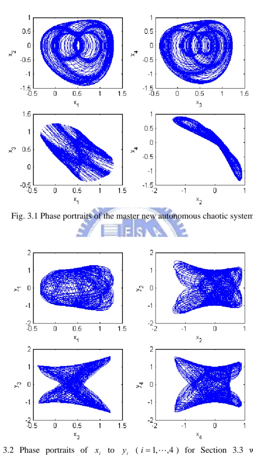
b= , (d) chaotic for b=1……….14 Fig. 2.5 Bifurcation diagram of the new nonautonomous chaotic system………...15 Fig. 2.6 Lyapunov exponents of the new nonautonomous chaotic system, where the sum of Lyapunov exponents is represented as a doted line at -1...……… 15 Fig. 3.1 Phase portraits of the master new autonomous chaotic system..…………28 Fig. 3.2 Phase portraits of x to _i y (_i i=1, , 4) for Section 3.3 when the

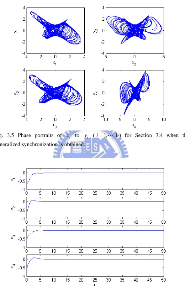
generalized synchronization is obtained……….…28 Fig. 3.3 Time histories of the state errors for Section 3.3..………..29 Fig. 3.4 Phase portraits of the master new nonautonomous chaotic system………29 Fig. 3.5 Phase portraits of x to _i y (_i i=1, , 4) for Section 3.4 when the

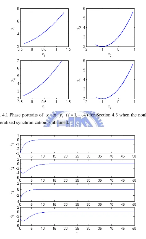
generalized synchronization is obtained.………30 Fig. 3.6 Time histories of the state errors for Section 3.4.……….. 30 Fig. 4.1 Phase portraits of x to _i y (_i i=1, , 4) for Section 4.3 when the

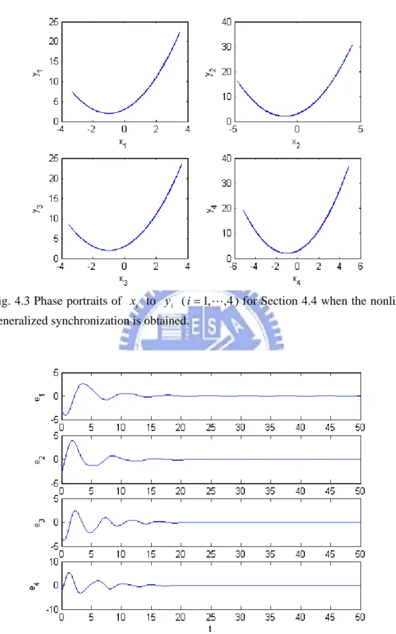
generalized synchronization is obtained.………47 Fig. 4.2 Time histories of the state errors for Section 4.3..………..47 Fig. 4.3 Phase portraits of x to _i y (_i i=1, , 4) for Section 4.4 when the

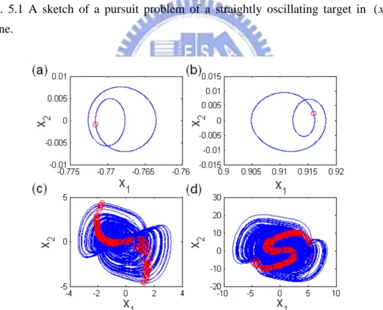
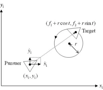
generalized synchronization is obtained.………48 Fig. 4.4 Time histories of the state errors for Section 4.4..………..48 Fig. 5.1 A sketch of a pursuit problem of a straightly oscillating target in ( ,x y _{1 1}) plane………... 58 Fig. 5.2 Phase portraits and Poincaré maps for straightly oscillating target pursuit

1.0

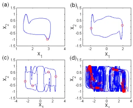
b= , (d) chaotic for b=1.8………..58 Fig. 5.3 Bifurcation diagram for straightly oscillating target pursuit problem...59 Fig. 5.4 Lyapunov exponents for straightly oscillating target pursuit problem…...59 Fig. 5.5 A sketch of a pursuit problem of a circularly rotating target in ( ,x y _{1 1}) plane………... 60 Fig. 5.6 Phase portraits and Poincaré maps for circularly rotating target pursuit

problem: (a) period 1 for b=0.2, (b) period 2 for b=0.58, (c) chaotic for b=0.78, (d) chaotic for b=0.81...………60 Fig. 5.7 Bifurcation diagram for circularly rotating target pursuit problem………61 Fig. 5.8 Lyapunov exponents for circularly rotating target pursuit problem...……61 Fig. 6.1 Phase portraits and Poincaré maps for nonlinear nonholonomic system

where the magnitude of velocity keeping constant: (a) period 1 for b=5.8, (b) period 2 for b=2.5, (c) period 4 for b=4.1, (d) chaotic for

5.3

b= ………....68

Fig. 6.2 Lyapunov exponents for nonlinear nonholonomic system where the magnitude of velocity keeping constant……… 68 Fig. 6.3 Largest Lyapunov exponent for nonlinear nonholonomic system where the magnitude of velocity keeping constant……….………69 Fig. 6.4 Bifurcation diagram for nonlinear nonholonomic system where the

magnitude of velocity keeping constant...………..69 Fig. 6.5 Period-doubling phenomenon for nonlinear nonholonomic system where

the magnitude of velocity keeping constant...…..………..………70 Fig. 7.1 The chaotic attractor of the van der Pol system for τ =2t+sint…... 84 Fig. 7.2 The chaotic attractor of uncontrolled forced nonlinear damped Mathieu

system……….84 Fig. 7.3 The chaotic attractor of the controlled forced nonlinear damped Mathieu

system...85 Fig. 7.4 Time histories of the state errors for Section 7.3 by applying method 1....85 Fig. 7.5 Time histories of the state errors for Section 7.3 by applying method 2....86 Fig. 7.6 Time histories of ˆL for Section 7.3.……… 86 Fig. 7.7 The chaotic attractor of the forced nonlinear damped Mathieu system for

5t

τ = ………..………87

Fig. 7.9 The chaotic attractor of the controlled Rössler system……….. 88

Fig. 7.10 Time histories of the state errors for Section 7.4 by applying method 1…88 Fig. 7.11 Time histories of the state errors for Section 7.4 by applying method 2…89 Fig. 7.12 Time histories of ˆL for Section 7.4...……….. 89

Fig. 8.1 The chaotic attractor of the Duffing system...………98

Fig. 8.2 The chaotic attractor of uncontrolled forced nonlinear damped Mathieu system...………..…....…98

Fig. 8.3 The chaotic attractor of the controlled forced nonlinear damped Mathieu system...………..…....99

Fig. 8.4 Time histories of the state errors for Section 8.3………....…99

Fig. 8.5 The chaotic attractor of the Lorenz system………..…… 100

Fig. 8.6 The chaotic attractor of uncontrolled Rössler system..………..….. 100

Fig. 8.7 The chaotic attractor of the controlled Rössler system..………..… 101

Chapter 1

Introduction

Chaotic phenomena have been observed in physics, chemistry, physiology, and many disciplines [1-3]. In contrast with the famous chaotic systems, such as Lorenz system, Duffing system, and Rössler system, nonlinear Mathieu system is less mentioned [4-9]. However, nonlinear Mathieu system is important and can be applied in analysis of the resonant micro electro mechanical systems [10-12]. In this thesis, the new autonomous and new nonautonomous chaotic systems constructed by mutual linear coupling of two non-identical nonlinear damped Mathieu systems are studied.

Chaos synchronization has been widely applied in secure communication [13, 14], biological systems [15, 16], and many other fields [17, 18]. The generalized synchronization is a complex type of chaos synchronization and gives rise to extensive investigations recently [19-26]. The mixed error dynamics and the plain square sum Lyapunov function are currently applied in studying the generalized synchronization, but there are some shortcomings and restrictions in them. The auxiliary numerical simulation is unavoidable for current mixed error dynamics in which master state variables and slave state variables are presented while their maximum values must be determined by simulation [27-31]. However, the pure error dynamics can be analyzed theoretically without additional numerical simulation. Besides, monotonous and self-limited square sum Lyapunov function, V e eTe

2 1 )

( = ,

is always used in most literatures [32-37], but the Lyapunov function can be chosen in a variety of elaborate and ingenious forms for different systems. Restricting Lyapunov function to square sum makes a long river brooklike, deeply weakens the powerfulness of Lyapunov direct method. Instead of current plain square sum

Lyapunov function, the elaborate Lyapunov function is applied in this thesis. A systematic method of designing Lyapunov function is proposed based on the Lyapunov direct method [38]. The generalized synchronization is achieved for both new autonomous and nonautonomous chaotic systems by applying this technique.

Since Hertz [39] distinguished nonholonomic system from holonomic system in 1894, the study of nonholonomic system [40, 41] has been developed over one hundred years. A great number of studies in this field are connected with the extension of the developed analytical methods for holonomic system and for the systems with nonholonomic constraints. At present the dynamics of nonholonomic system has many applications in the problems of modern technology, such as the pursuit problems, the motion of automobiles, landing devices of airplanes, railway wheels, etc. However, the complete study of chaos in nonholonomic systems remains deficient. As far as we know, the only paper studies the chaos of nonholonomic system with an external constraint is Ref. [42], in which the chaotic phenomena of rattleback dynamics are studied. But in this paper, only Poincaré maps are given. As it is well-known, the only Poincaré map can not identify the existence of chaos reliably.

The moving target pursuit problem [43] is a typical example of nonholonomic system. In this thesis, chaos of nonholonomic systems with external nonholonomic constraint for two types of pursuit problems, a straightly oscillating target, and a circularly rotating target, is studied by applying the fundamental nonholonomic form of Lagrange’s equations [44, 45]. Moreover, chaos of nonholonomic system with external nonlinear nonholonomic constraint, the magnitude of velocity keeping constant, is studied in this thesis by applying the nonlinear nonholonomic form of Lagrange’s equations. All numerical criteria of chaos, i.e. the most reliable Lyapunov exponents [46], phase portraits, Poincaré maps and bifurcation diagrams are firstly

nonholonomic systems. Furthermore, it is found that the Feigenbaum number rule [47] still holds for nonlinear nonholonomic system.

There are various types of synchronization, such as complete synchronization [48], generalized synchronization [49], phase synchronization [50], lag synchronization [51], and so on. Among these types of synchronization, generalized synchronization is one of the most interesting topics. Generalized synchronization refers to a functional relation between the state vectors of master and slave, i.e.

( , )t =

y F x , where x and y are the state vectors of master and slave. In the work of Ref. [52], the generalized synchronization is extended to a more general form,

( , , )t =

y F x y , where the “slave” y is not a traditional pure slave obeying the “master” x completely but plays a role to determine the final desired state of the “slave”. Since the “slave” y plays an “interwined” role, this type of synchronization is called “symplectic synchronization”1, the master is called “partner A”, and the slave is called “partner B”. In this thesis, we propose two types of new chaos synchronization, “non-simultaneous symplectic synchronization” and “double symplectic synchronization”.

We propose the “non-simultaneous symplectic synchronization”, ( )t = ( ( ), ( ), )τ t t

y F x y , where τ is a given function of time t , so-called variable scale time. The synchronization is achieved at “different time” for “partner A” ( )xτ and “partner B” ( )y t , therefore we call this type of synchronization “non-simultaneous symplectic synchronization”. When τ = , non-simultaneous t symplectic synchronization reduces to symplectic synchronization. When applying the non-simultaneous symplectic synchronization in secret communication, since the functional relation of the non-simultaneous symplectic synchronization is more

1 _{The term ‘‘symplectic’’ comes from the Greek for ‘‘interwined’’. H. Weyl first introduced the term in 1939} in his book “The Classical Groups” (p. 165 in both the first edition, 1939, and second edition, 1946, Princeton University Press).

complex than that of the traditional generalized synchronization, and cracking the variable scale time τ is an extra task for the attackers in addition to cracking the system model and cracking the functional relation, the message is harder to be detected by applying the non-simultaneous symplectic synchronization than by applying traditional generalized synchronization. Therefore, the non-simultaneous symplectic synchronization may be applied to increase the security of secret communication. In order to achieve non-simultaneous symplectic synchronization, nonlinear control [53] and adaptive control are applied. In the work of Ref. [53], the induced matrix norm and the Lipschitz constant are obtained by auxiliary numerical simulation. However, they can be estimated theoretically by using the property of induced matrix norms [54a] and by applying adaptive control. Furthermore, in our case, non-simultaneous symplectic synchronization, the complexity of the functional relation ( ( ), ( ), )F xτ y t t is greater than that studied in Ref. [53], thus the Lipschitz constant may be enormous. However, by applying adaptive control, the estimated Lipschitz constant is much less than the Lipschitz constant obtained by applying nonlinear control. This result in the reduction of the gain of the controller, i.e. the cost of controller is reduced. The proposed scheme is effective and feasible for both autonomous and nonautonomous chaotic systems, whether the dimensions of ( )xτ and ( )y t systems are the same or not.

Finally, the “double symplectic synchronization”, G x y( , )=F x y( , , )t , is proposed. Since the symplectic functions are presented at both the right hand side and the left hand side of the equality, it is called “double symplectic synchronization”. It is an extension of symplectic synchronization, y F x y= ( , , )t . When G x y( , )=y , the double symplectic synchronization is reduced to the symplectic synchronization. Due to the complexity of the form of the double symplectic synchronization, it may be

synchronization is obtained by applying active control. A scheme of synchronization is derived based on Barbalat’s lemma [54b], and it is effective and feasible for both autonomous and nonautonomous chaotic systems.

The contents of this thesis are as follows. Chapter 2 contains the dynamics of new autonomous and nonautonomous chaotic systems. The system models are described and the numerical results of regular and chaotic behaviors are presented. In Chapter 3, generalized synchronization of new chaotic systems is achieved by applying pure error dynamics and elaborate Lyapunov function. The methods of designing Lyapunov function are presented, and both new autonomous and new nonautonomous chaotic systems are illustrated in examples. By applying pure error dynamics and elaborate nondiagonal Lyapunov function, nonlinear generalized synchronization of new chaotic systems is obtained in Chapter 4. We propose the methods of designing Lyapunov function, and illustrate them by both new autonomous and new nonautonomous chaotic systems in examples. In Chapter 5, the dynamics of nonholonomic systems is studied by applying the fundamental nonholonomic form of Lagrange’s equations. Two types of external nonholonomic constraints are studied for moving target pursuit problems: a straightly oscillating target and a circularly rotating target. Numerical results show that chaos exists in each case. By applying the nonlinear nonholonomic form of Lagrange’s equations, the dynamics of nonlinear nonholonomic system is studied in Chapter 6. We investigate external nonlinear nonholonomic constraint: the magnitude of velocity keeping constant. Chaos is proved to exist in each case by numerical results. Furthermore, Feigenbaum number rule still holds for nonlinear nonholonomic system. In Chapter 7, the non-simultaneous symplectic synchronization is proposed, and it is achieved by applying adaptive control. The synchronization scheme is presented, and chaotic systems with the same or different dimensions are illustrated in examples. We

investigate the double symplectic synchronization by applying active control in Chapter 8. The synchronization scheme is derived, and both autonomous and nonautonomous chaotic systems are illustrated in examples. Finally, the conclusions of the whole thesis are drawn in Chapter 9.

References

[1] F. C. Moon, Chaotic and fractal dynamics: an introduction for applied scientists and engineers, Second Edition, Wiley, New York, 1992.

[2] E. Ott, Chaos in Dynaimical Systems, Second Edition, Cambridge University Press, New York, 2002.

[3] J. M. T. Thompson and H. B. Steward, Nonlinear Dynamics and Chaos, Second Edition, John Wiley & Sons, New York, 2002.

[4] M. Mond, G. Cederbaum, P. B. Khan, and Y. Zarmi, “Stability Analysis Of The Non-Linear Mathieu Equation”, Journal of Sound and Vibration, 1993, Vol. 167, pp. 77-89.

[5] J. W. Norris, “The Nonlinear Mathieu Equation”, International Journal of Bifurcation and Chaos, 1994, Vol. 4, pp. 71-86.

[6] Y. O. El-Dib, “Nonlinear Mathieu Equation and Coupled Resonance Mechanism”, Chaos, Solitons and Fractals, 2001, Vol. 12, pp. 705-720.

[7] L. Ng and R. Rand, “Bifurcations in a Mathieu Equation with Cubic Nonlinearities”, Chaos, Solitons and Fractals, 2002, Vol. 14, pp. 173-181.

[8] Z. M. Ge and C. X. Yi, “Chaos in a Nonlinear Damped Mathieu System, in a Nano Resonator System and Its Fractional Order Systems”, Chaos, Solitons and Fractals, 2007, Vol. 32, pp. 42-61.

[9] Z. M. Ge and C. X. Yi, “Parameter Excited Chaos Synchronization of Integral and Fractional Order Nano Resonator System”, Mathematical Mehtods, Physical Models and Simulation in Science and Technology, 2006, Vol. 1, pp.239-265. [10] R. Baskaran and K. L. Turner, “Mechanical Domain Coupled Mode Parametric

Resonance and Amplification in a Torsional Mode Micro Electro Mechanical Oscillator”, Journal of Micromechanics and Microengineering, 2001, Vol. 13, pp. 701-707.

[11] N. Mahmoudian, M. R. Aagaah, G. N. Jazar and M. Mahinfalah, “Dynamics of a Micro Electro Mechanical Systems (MEMS)”, Proceedings of the 2004 International Conference on MEMS, NANO and Smart Systems, 2004, pp. 688-693.

[12] M. Napoli, R. Baskaran, K. L. Turner, and B. Bamieh, “Understanding Mechanical Domain Parametric Resonance in Microcantilevers”, IEEE the 16th Annual International Conference on MEMS, 2003, pp. 169-172.

[13] K. M. Cuomo and V. Oppenheim, “Circuit Implementation of Synchronized Chaos with Application to Communication”, Physical Review Letters, 1993, Vol. 71, pp. 65-68.

[14] L. Kocarev and U. Parlitz, “General Approach for Chaotic Synchronization with Application to Communication”, Physical Review Letters, 1995, Vol. 74, pp. 5028-5031.

[15] S. K. Han, C. Kerrer, and Y. Kuramoto, “Dephasing and Bursting in Coupled Neural Oscillators”, Physical Review Letters, 1995, Vol. 75, pp. 3190-3193.

[16] B. Blasius, A. Huppert, and L. Stone, “Complex Dynamics and Phase Synchronization in Spatially Extended Ecological Systems”, Nature, 1999, Vol. 399, pp. 354-359.

[17] H. K. Chen and T. N. Lin, “Synchronization of Chaotic Symmetric Gyros by One-Way Coupling Conditions”, Journal of Mechanical Engineering Science, 2003, Vol. 217, pp. 331-340.

[18] Z. M. Ge and C. M. Chang, “Chaos Synchronization and Parameter Identification for Single Time Scale Brushless DC Motor”, Chaos, Solitons and Fractals, 2004, Vol. 20, pp. 889-903.

[19] N. F. Rulkov, M. M. Sushchik, L. S. Tsimring, and H. D. I. Abarbanel, “Generalized Synchronization of Chaos in Directionally Coupled Chaotic Systems”, Physical Review E, 1995, Vol. 51, pp. 980-994.

[20] H. D. I. Abarbanel, N. F. Rulkov, and M. M. Sushchik, “Generalized Synchronization of Chaos: The Auxiliary System Approach”, Physical Review E, 1996, Vol. 53, pp. 4528-4535.

[21] S. S. Yang and C. K. Duan, “Generalized Synchronization in Chaotic Systems”, Chaos, Solitons and Fractals, 1998, Vol. 9, pp. 1703-1707.

[22] M. Inoue, T. Kawazoe, Y. Nishi, and M. Nagadome, “Generalized Synchronization and Partial Synchronization in Coupled Maps”, Physics Letters A, 1998, Vol. 249, pp. 69-73.

[23] J. R. Terry and G. D. VanWiggeren, “Chaotic Communication Using Generalized Synchronization”, Chaos, Solitons and Fractals, 2001, Vol. 12, pp. 145-152.

[24] J. G. Lu and Y. G. Xi, “Linear Generalized Synchronization of Continuous-Time Chaotic Systems”, Chaos, Solitons and Fractals, 2003, Vol. 17, pp. 825-831. [25] A. E. Hramov and A. A. Koronovskii, “Generalized Synchronization: A Modified

System Approach”, Chaos, Solitons and Fractals, 2005, Vol. 71, pp. 067201-067204.

[26] Y. W. Wang and Z. H. Guan, “Generalized Synchronization of Continuous Chaotic System”, Physical Review E, 2006, Vol. 27, pp. 97-101.

[27] G. P. Jiang and W. K. S. Tang, “A Global Synchronization Criterion for Coupled Chaotic Systems via Unidirectional Linear Error Feedback”, International Journal of Bifurcation and Chaos, 2002, Vol. 12, pp. 2239-2253.

Synchronization Using Linear State Feedback Control”, International Journal of Bifurcation and Chaos, 2003, Vol. 13, pp. 2343-2351.

[29] G. P. Jiang, W. K. S. Tang, and G. R. Chen, “A Simple Global Synchronization Criterion for Coupled Chaotic Systems”, Chaos, Solitons and Fractals, 2003, Vol. 15, pp. 925-935.

[30] J. Sun and Y. Zhang, “Some Simple Global Synchronization Criterions for Coupled Time-varying Chaotic Systems”, Chaos, Solitons and Fractals, 2004, Vol. 19, pp. 93-98.

[31] E. M. Elabbasy, H. N. Agiza and M. M. El-Dessoky, “Global Synchronization Criterion and Adaptive Synchronization for New Chaotic System”, Chaos, Solitons and Fractals, 2005, Vol. 23, pp. 1299-1309.

[32] M. T. Yassen, “Controlling, Synchronization and Tracking Chaotic Liu System Using Active Backstepping Design”, Physics Letters A, 2007, Vol. 360, pp. 582-587.

[33] S. A. Lazzouni, S. Bowong, F.M. M. Kakmeni, and B. Cherki, “An Adaptive Feedback Control for Chaos Synchronization of Nonlinear Systems with Different Order”, Communications in Nonlinear Science and Numerical Simulation, 2007, Vol. 12, pp. 568-583.

[34] W. W. Yu and J. D. Cao, “Adaptive Synchronization and Lag Synchronization of Uncertain Dynamical System with Time Delay Based on Parameter Identification”, Physica A, 2007, Vol. 375, pp. 467-482.

[35] E. M. Elabbasy, H. N. Agiza, and M. M. El-Dessoky, “Adaptive Synchronization of a Hyperchaotic System with Uncertain Parameter”, Chaos, Solitons and Fractals, 2006, Vol. 30, pp. 1133-1142.

[36]J. X. Wang, D. C. Lu, and L. X. Tian, “Global Synchronization for Time-Delay of WINDMI System”, Chaos, Solitons and Fractals, 2006, Vol. 30, pp. 629-635. [37] C. P. Li and J. P. Yan, “Generalized Projective Synchronization of Chaos: The

Cascade Synchronization Approach”, Chaos, Solitons and Fractals, 2006, Vol. 30, pp. 140-146.

[38] J. J. E. Slotine and W. Li, Applied Nonlinear Control, Prentice-Hall, New Jersey, 1991.

[39] H. R. Hertz, Die Prinzipien der Mechanik in neuem Zusammenhange dargestellt, Barth, Leipzig, 1894.

[40] F. Mei, “Nonholonomic Mechanics”, Applied Mechanics Reviews, 2000, Vol. 53, pp. 283-305.

[41] I. Kolmanovsky and N. H. McClamroch, “Developments in Nonholonomic Control Problems”, IEEE Control System Magazine, 1995, Vol. 15, pp. 20-36. [42] A. V. Borisov and I. S. Mamaev, “Strange Attractors in Rattleback Dynamics”,

Physics Uspekhi, 2003, Vol. 46, pp. 393-403.

[43] L. A. Pars, A Treatise on Analytical Dynamics, Heinemann, London, 1965, pp. 17-18.

[44] H. Goldstein, C. Poole and J. Safko, Classical Mechanics, Third Edition, Addison Wesley, San Francisco, 2002, p. 20.

[45] D. T. Greenwood, Advanced Dynamics, Cambridge University Press, Cambridge, 2003, pp. 73-80.

[46] S. Wiggins, Introduction to Applied Nonlinear Dynamical Systems and Chaos, Second Edition, Springer, New York, 2003, pp. 726-730.

[47] M. J. Feigenbaum, “Quantitative Universality for a class of nonlinear transformations”, Journal of Statistical Physics, 1978, Vol. 19, pp. 25-32.

[48] L. M. Pecora and T. L. Carroll, “Synchronization in chaotic system”, Physical Review Letters, 1990, Vol. 64, pp. 821–824.

[49] N. F. Rulkov, M. M. Sushchik, L. S. Tsimring, and H. D. I. Abarbanel, “Generalized synchronization of chaos in directionally coupled chaotic systems”, Physical Review E, 1995, Vol. 51, pp. 980-994.

[50] M. G. Rosenblum, A. S. Pikovsky, and J. Kurths, “Phase Synchronization of Chaotic Oscillators”, Physical Review Letters, 1996, Vol. 76, pp. 1805-1807. [51] M. G. Rosenblum, A. S. Pikovsky, and J. Kurths, “From Phase to Lag

Synchronization in Coupled Chaotic Oscillators”, Physical Review Letters, 1997, Vol. 78, pp. 4193-4196.

[52] Z. M. Ge and C. H. Yang, “Symplectic Synchronization of Different Chaotic Systems”, Chaos, Solitons and Fractals, 2009, Vol. 40, pp. 2536-2543.

[53] J. Meng and X. Y. Wang, “Generalized Synchronization via Nonlinear Control”, Chaos, 2008, Vol. 18, pp. 023108-1-023108-5.

[54a] H. K. Khalil, Nonlinear Systems, Third Edition, Prentice Hall, New Jersey, 2002, p. 648.

[54b] H. K. Khalil, Nonlinear Systems, Third Edition, Prentice Hall, New Jersey, 2002, p. 323.

Chapter 2

Regular and Chaotic Dynamics of New Chaotic Systems

The nonlinear Mathieu system [1-6] is important and can be applied in analysis of the resonant micro electro mechanical systems [7-9]. In this Chapter, we propose new autonomous and new nonautonomous chaotic systems constructed by mutual linear coupling of two non-identical nonlinear damped Mathieu systems.

Consider two non-identical nonlinear damped Mathieu systems [5, 6] described by 1 2 3 2 1 1 2 , (1 sin ) (1 sin ) , x x x a ωt x ωt x ax = = − + − + − (2.1) 3 4 3 4 3 3 4 , (1 sin ) (1 sin ) , x x x ωt x a ωt x ax = = − + − + − (2.2)

where a and ω are constants.

A new autonomous chaotic system can be constructed by mutual linear coupling of two non-identical nonlinear damped Mathieu systems, Eq. (2.1) and Eq. (2.2). The term sin tω of one Mathieu system is replaced by one state of the other Mathieu

system, and linear coupling terms are added to each other:

1 2 3 2 4 1 4 1 2 3 3 4 3 4 2 3 2 3 4 1 , (1 ) (1 ) , , (1 ) (1 ) . x x x a x x x x ax bx x x x x x a x x ax bx = = − + − + − + = = − + − + − + (2.3)

The parameters in simulation are a=0.5,b=1~1.254, and the initial condition is . 2 . 0 ) 0 ( , 2 . 0 ) 0 ( , 1 . 0 ) 0 ( , 1 . 0 ) 0 ( 2 3 4 1 = x = x = x =

x The phase portraits, Poincaré maps,

are shown in Fig. 2.1-2.3. It can be observed that the motion is period 1 for b=1.1, period 4 for b=1.243, and period 8 for b=1.246. For b=1.24, the motion is chaotic.

A new nonautonomous chaotic system can also be constructed by mutual linear coupling of two non-identical nonlinear damped Mathieu systems, Eq. (2.1) and Eq. (2.2). The terms sin tω of each Mathieu system are preserved, and linear coupling

terms are added to each other:

1 2 3 2 1 1 2 3 3 4 3 4 3 3 4 1 , (1 sin ) (1 sin ) , , (1 sin ) (1 sin ) . x x x a ωt x ωt x ax bx x x x ωt x a ωt x ax bx = = − + − + − + = = − + − + − + (2.4)

The parameters in simulation are a=0.5,b=0.9~1,ω=1, and the initial condition is .x₁(0)=0.1,x₂(0)=0.1,x₃(0)=0.2,x₄(0)=0.2 The phase portraits, Poincaré maps, bifurcation diagram, and Lyapunov exponents of the new nonautonomous chaotic system are shown in Fig. 2.4-2.6. It can be observed that the motion is period 1 for b=0.9, period 2 for b=0.93, and period 4 for b=0.934. For b=1, the motion is chaotic.

Fig. 2.1 Phase portraits and Poincaré maps of the new autonomous chaotic system: (a) period 1 for b=1.1, (b) period 4 for b=1.243, (c) period 8 for b=1.246, (d) chaotic for b=1.24.

Fig. 2.3 Lyapunov exponents of the new autonomous chaotic system, where the sum of Lyapunov exponents is represented as a doted line at -1.

Fig. 2.4 Phase portraits and Poincaré maps of the new nonautonomous chaotic system: (a) period 1 for b=0.9, (b) period 2 for b=0.93, (c) period 4 for b=0.934, (d) chaotic for b=1.

Fig 2.5 Bifurcation diagram of the new nonautonomous chaotic system.

Fig. 2.6 Lyapunov exponents of the new nonautonomous chaotic system, where the sum of Lyapunov exponents is represented as a doted line at -1.

References

[1] M. Mond, G. Cederbaum, P. B. Khan, and Y. Zarmi, “Stability Analysis Of The Non-Linear Mathieu Equation”, Journal of Sound and Vibration, 1993, Vol. 167, pp. 77-89.

[2] J. W. Norris, “The Nonlinear Mathieu Equation”, International Journal of Bifurcation and Chaos, 1994, Vol. 4, pp. 71-86.

[3] Y. O. El-Dib, “Nonlinear Mathieu Equation and Coupled Resonance Mechanism”, Chaos, Solitons and Fractals, 2001, Vol. 12, pp. 705-720.

[4] L. Ng and R. Rand, “Bifurcations in a Mathieu Equation with Cubic Nonlinearities”, Chaos, Solitons and Fractals, 2002, Vol. 14, pp. 173-181.

[5] Z. M. Ge and C. X. Yi, “Chaos in a Nonlinear Damped Mathieu System, in a Nano Resonator System and Its Fractional Order Systems”, Chaos, Solitons and Fractals, 2007, Vol. 32, pp. 42-61.

[6] Z. M. Ge and C. X. Yi, “Parameter Excited Chaos Synchronization of Integral and Fractional Order Nano Resonator System”, Mathematical Mehtods, Physical Models and Simulation in Science and Technology, 2006, Vol. 1, pp.239-265. [7] R. Baskaran and K. L. Turner, “Mechanical Domain Coupled Mode Parametric

Resonance and Amplification in a Torsional Mode Micro Electro Mechanical Oscillator”, Journal of Micromechanics and Microengineering, 2001, Vol. 13, pp. 701-707.

[8] N. Mahmoudian, M. R. Aagaah, G. N. Jazar and M. Mahinfalah, “Dynamics of a Micro Electro Mechanical Systems (MEMS)”, Proceedings of the 2004 International Conference on MEMS, NANO and Smart Systems, 2004, pp. 688-693.

[9] M. Napoli, R. Baskaran, K. L. Turner, and B. Bamieh, “Understanding Mechanical Domain Parametric Resonance in Microcantilevers”, IEEE the 16th Annual International Conference on MEMS, 2003, pp. 169-172.

Chapter 3

Generalized Synchronization of New Chaotic Systems by

Pure Error Dynamics and Elaborate Lyapunov Function

3.1 Preliminaries

In this Chapter, the generalized synchronization is studied by applying pure error dynamics and elaborate Lyapunov function. The pure error dynamics can be analyzed theoretically without auxiliary numerical simulation, whereas the aid of additional numerical simulation is unavoidable for current mixed error dynamics in which master state variables and slave state variables are presented while their maximum values must be determined by simulation [1-5]. Besides, the elaborate Lyapunov function is applied rather than current plain square sum Lyapunov function,

e e e T V 2 1 )

( = , which is currently used [6-11] for convenience. However, Lyapunov

function can be chosen in a variety of forms for different systems. Restricting Lyapunov function to square sum makes a long river brooklike, deeply weakens the powerfulness of Lyapunov direct method. Based on Lyapunov direct method [12], the generalized synchronization is achieved and a systematic method of designing Lyapunov function is proposed.

3.2 Design of Lyapunov Function

Consider the master and slave nonlinear dynamic systems described by ( , )t = x f x , (3.1) ( , )t ( , , )t = + y f y u x y , (3.2)

where x,y∈Rn are master and slave state vectors, f :R₊×Rn →Rn is a nonlinear vector function, and u: R₊×Rn×Rn →Rn is controller vector.

Generalized synchronization means that there is a functional relation y=g( xt, ) between master and slave states as time goes to infinity, where g:R₊×Rn →Rn is a continuously differentiable vector function. Define e=y−g( xt, ) as generalized synchronization error vector, and the error dynamics can be obtained:

( , ) ( , ) ( , ) ( , ) ( , ) ( , ) ( , ) ( , , ). t t t t t t t t t t = − ∂ ∂ = − − ∂ ∂ ∂ ∂ = − − + ∂ ∂ e y g x g x g x y x x g x g x f y f x u x y x (3.3)

Based on Lyapunov direct method [12], the scheme of generalized synchronization and the procedure of designing Lyapunov function are described as follows:

Step 1. Construct a Lyapunov function

2 2 2 11 1 22 2 1 1 1 1 ( , ) ( ) ( ) ( ) ( ) 2 2 2 2 T nn n V t e = e Λ et = λ t e + λ t e + + λ t e , (3.4)

where Λ( )t =[λ_ii( )]t ∈Rn n× is an unknown continuously differentiable positive definite diagonal matrix to be designed. Its derivative is

11 1 1 22 2 2 2 2 2 11 1 22 2 1 ( , ) ( ) ( ) 2 ( ) ( ) ( ) 1 1 1 ( ) ( ) ( ) . 2 2 2 T T nn n n nn n V t t t t e e t e e t e e t e t e t e λ λ λ λ λ λ = + = + + + + + + + e e Λ e e Λ e (3.5)

Step 2. Eq. (3.5) can be rewritten in the following form:

2 2 2 1 11 11 1 2 22 22 2 1 11 1 1 11 1 1 2 11 1 1 22 2 2 11 1 1 ( , ) ( , ) ( , ) ( , ) [ ( , , , , , , , , , ) ] [ ( , , , , , , , , , ) ] [ ( , , , , , , , , , ) ] , n nn nn n nn n n nn n n n nn n n nn n n V t G e G e G e H x x y y t u e H x x y y t u e H x x y y t u e λ λ λ λ λ λ λ λ λ λ λ λ λ λ λ = + + + + + + + + + + e (3.6)

where )G_i(λ_ii,λ_ii and H_i(λ₁₁, ,λ_nn,x₁, ,x_n,y₁, ,y_n,t) (i=1,2, ,n) are continuous differentiable functions, u_i (i=1,2, ,n) are controllers to be determined.

Step 3. Eq. (3.6) may be classified as two general forms: (1) All G_i(λ_ii,λ_ii) depend on )λ_ii(t and λ_ii(t), (2) Some of G_j(λ_jj,λ_jj) depend on λ_jj(t) and λ_jj(t), the

remaining )G_k(λ_kk,λ_kk depend only on λ_kk(t).

Form (1): All G_i(λ_ii,λ_ii) depend on λ_ii(t) and λ_ii(t). Step 4. Design the controllers u such that _i

11 1 1

( , , , , , , , , , ) 0 ( 1, 2, , )

i nn n n ii i

H λ λ x x y y t +λ u = i= n , (3.7)

i.e. current mixed error dynamics has been replaced by pure error dynamics. By Eq. (3.7), we design the controllers u such that _i λ_ii (i=1,2, ,n) are linear function of each other with positive coefficients.

Step 5. Design )λ₁₁(t),λ₂₂(t), ,λ_nn(t such that 0, 0 _{mii ii}( ) _{M ii} ( 1, 2, , )

t λ λ t λ i n

∀ ≥ < ≤ ≤ = , (3.8)

where λ_mii, λ_Mii are positive constants, and

0, _i( _ii, _ii) 0 ( 1, 2, , )

t G λ λ i n

∀ ≥ < = , (3.9)

then the Lyapunov function can be obtained and the generalized synchronization is achieved according to Lyapunov direct method.

Form (2): Some of G_j(λ_jj,λ_jj) depend on λ_jj(t) and λ_jj(t) , and the

remaining )G_k(λ_kk,λ_kk depend only on λ_kk(t). Step 4. Assume

, _kk( ) 1 k λ t ∀ = , (3.10) 11 1 1 , _k( , , _nn, , , _n, , , _n, ) _kk( ) _{k k} k H λ λ x x y y t λ t u e ∀ + = − , (3.11) 11 1 1 , _j( , , _nn, , , _n, , , _n, ) _jj( ) _j 0 j H λ λ x x y y t λ t u ∀ + = , (3.12)

i.e. current mixed error dynamics has been replaced by pure error dynamics, and appropriately design the controllers u_i (i=1,2, ,n) and λ_jj(t) such that

0, 0 _{m jj jj}( ) _{M jj}

t λ λ t λ

∀ ≥ < ≤ ≤ , (3.13)

where λ_{m jj}, λ_{M jj} are positive constants, and

0, j( jj, jj) 0

t G λ λ

∀ ≥ < , (3.14)

then the Lyapunov function can be obtained and the generalized synchronization is achieved according to Lyapunov direct method.

3.3 Example for New Autonomous Chaotic Systems

In the following two Sections, the functional relation between master and slave states is y_i = g_i(t,x_i)=α(t)x_i +β(t) (i=1,2, ,n).

The new autonomous chaotic system is constructed by mutual linear coupling of two non-identical nonlinear damped Mathieu systems, and the master and slave new autonomous chaotic systems can be described by

1 2 3 2 4 1 4 1 2 3 3 4 3 4 2 3 2 3 4 1 , (1 ) (1 ) , , (1 ) (1 ) , x x x a x x x x ax bx x x x x x a x x ax bx = = − + − + − + = = − + − + − + (3.15)

1 2 1 3 2 4 1 4 1 2 3 2 3 4 3 3 4 2 3 2 3 4 1 4 , (1 ) (1 ) , , (1 ) (1 ) . y y u y a y y y y ay by u y y u y y y a y y ay by u = + = − + − + − + + = + = − + − + − + + (3.16)

The parameters in simulation are a=0.5, b=1.24, and the initial condition is

1 . 0 ) 0 ( 1 = x , x₂(0)=0.1, 2x₃(0)=0. , x₄(0)=0.2 , y₁(0)=0.3 , y₂(0)=0.3, 3(0) 0.4

y = , y₄(0)=0.4. The phase portraits of the master new autonomous chaotic system are shown in Fig. 3.1.

Let )e_i = y_i −α(t)x_i −β(t) (i=1, ,4 , then the error dynamics can be obtained: 1 2 1 1 3 3 2 1 2 3 1 4 1 4 4 1 4 1 2 2 3 4 3 3 3 4 3 4 1 2 3 2 3 2 3 2 ( ) ( ) ( ) , ( ( ) ) [(1 ) ( )(1 ) ] ( ) ( 2 ) ( ) ( ) , ( ) ( ) ( ) , ( ( ) ) [(1 ) ( )(1 ) e e t x t t u e ae ae be a y y t x x y y t x x t x b a t t u e e t x t t u e e ae be y y t x x a y y t x α β β α α α β β α β β α α = − + − + = − − + − − − + − + − + − − + = − + − + = − − + − − − + − + 3 3 4 4 ] ( ) ( 1) ( ) ( ) . x t x b a t t u α β β − + − − − + (3.17)

Step 1. Construct a Lyapunov function

2 2 2 2 11 1 22 2 33 3 44 4 1 1 1 1 1 ( , ) ( ) ( ) ( ) ( ) ( ) 2 2 2 2 2 T V t e = e Λ et = λ t e + λ t e + λ t e + λ t e . (3.18) Its derivative is 2 2 11 1 11 1 1 22 2 22 2 2 2 2 33 3 33 3 3 44 4 44 4 4 1 1 ( , ) ( ) ( ) ( ) ( ) 2 2 1 1 ( ) ( ) ( ) ( ) . 2 2 V t t e t e e t e t e e t e t e e t e t e e λ λ λ λ λ λ λ λ = + + + + + + + e (3.19)

2 2 2 2 1 11 11 1 2 22 22 2 3 33 33 3 4 44 44 4 1 11 44 1 4 1 4 11 1 1 2 11 44 1 4 1 4 22 2 2 3 11 44 1 4 1 4 33 3 3 ( , ) ( , ) ( , ) ( , ) ( , ) [ ( , , , , , , , , , ) ] [ ( , , , , , , , , , ) ] [ ( , , , , , , , , , ) ] [ V t G e G e G e G e H x x y y t u e H x x y y t u e H x x y y t u e H λ λ λ λ λ λ λ λ λ λ λ λ λ λ λ λ λ = + + + + + + + + + + e 4(λ11, ,λ44, ,x1 ,x y4, 1, ,y t4, )+λ44u e4] ,4 (3.20) where 1 11 11 11 11 2 22 22 22 22 3 33 33 33 33 4 44 44 44 44 1 11 11 1 1 44 4 2 11 11 1 22 1 1 ( , ) ( ) ( ), ( , ) ( ) ( ), 2 2 1 1 ( , ) ( ) ( ), ( , ) ( ) ( ), 2 2 ( , , ) ( )[ ( ) ( ) ( ) ] ( ) , ( , , ) ( ) ( G t t G t a t G t t G t a t H t t t x t t e b t e H t t e λ λ λ λ λ λ λ λ λ λ λ λ λ λ λ λ λ λ α β β λ λ λ λ = − = − = − = − = − + − + + = + 3 1 4 1 4 1 4 1 3 4 1 2 3 11 22 2 33 3 3 3 4 11 33 3 44 3 2 3 2 3 2 3 2 )[ ( ( ) ) ((1 ) ( )(1 ) ) ( ) ( 2 ) ( ) ( )], ( , , ) ( ) ( )[ ( ) ( ) ( ) ], ( , , ) ( ) ( )[ ( ( ) ) ((1 ) ( )(1 ) t ae a y y t x x y y t x x t x b a t t H t b t e t t x t t e H t t e t e y y t x x a y y t x α α α β β λ λ λ α β β λ λ λ α α − − − − + − + − + − − = + − + − + = + − − − − + − + 3 3) ( ) 4 ( 1) ( ) ( )]. x −α t x + − −b a β t −β t (3.21)

Step 3. Since all G_i(λ_ii,λ_ii) depend on λ_ii(t) and λ_ii(t) (i=1, ,4), Eq. (3.20) can be classified as form (1).

Step 4. Design the controllers

1 1 4 1 4 3 3 2 1 4 1 4 4 1 4 1 2 3 2 3 3 2 3 4 2 3 2 3 2 3 2 ( ( ) ( )) ( ) ( ) ( ), ( ( ) ) (1 ) ( )(1 ) ( ) ( 2 ) ( ) ( ), ( ( ) ( )) ( ) ( ) ( ), ( ) (1 ) ( )(1 ) u y by t t x b t x b t t u a y y t x x y y t x x t x b a t t u by y t t x b t x b t t u y y t x x a y y t x x α α α β β α α α β β α α α β β α α = − − + + + + + = − + + − + + − − + = − − + + + + + = − + + − + 3 3 3 3 4 1 1 1 (1 )y (1 ) ( )t x ( )t x (b a ) ( )t ( ),t a a α α a β β + − − − + − − − + (3.22) such that 11 44 1 4 1 4 ( , , , , , , , , , ) ( ) 0 ( 1, , 4) i ii i H λ λ x x y y t +λ t u = i= , (3.23)

11 44 22 11 33 11

1 1

( )t ( ),t ( )t ( ),t ( )t ( )t

a a

λ =λ λ = λ λ = λ . (3.24)

Now, the mixed error dynamics is replaced by pure error dynamics:

2 2 2 2 1 11 11 1 2 22 22 2 3 33 33 3 4 44 44 4 ( , ) ( , ) ( , ) ( , ) ( , ) V t e =G λ λ e +G λ λ e +G λ λ e +G λ λ e . (3.25) Step 5. Design 11 22 33 44 1 1 1 1 ( ) , ( ) , ( ) , ( ) 1 t (1 t) (1 t) 1 t t t t t e a e a e e λ = ₋ λ = ₋ λ = ₋ λ = ₋ + + + + , (3.26) such that 11 11 11 22 22 22 33 33 33 44 44 44 1 0, 0 ( ) ( ) ( ) 1, 2 1 1 0, 0 ( ) ( ) ( ) , 2 1 1 0, 0 ( ) ( ) ( ) , 2 1 0, 0 ( ) ( ) ( ) 1, 2 m M m M m M m M t t t t t t t t a a t t t t a a t t t t λ λ λ λ λ λ λ λ λ λ λ λ ∀ ≥ < = ≤ ≤ = ∀ ≥ < = ≤ ≤ = ∀ ≥ < = ≤ ≤ = ∀ ≥ < = ≤ ≤ = (3.27) 1 11 11 11 11 2 2 22 22 22 22 2 2 3 33 33 33 33 2 2 1 2 0, ( , ) ( ) ( ) 0, 2 2(1 ) 1 2 (1 2 ) 1 0, ( , ) ( ) ( ) 0, 2 2 (1 ) (1 ) 1 2 2 0, ( , ) ( ) ( ) 0, 2 2 (1 ) (1 ) 0, t t t t t t t t t e t G t t e a a e t G t a t a e e e e t G t t a e e t λ λ λ λ λ λ λ λ λ λ λ λ − − − − − − − − − − − ∀ ≥ = − = < + − + − − ∀ ≥ = − = = < + + − − − − ∀ ≥ = − = = < + + ∀ ≥ 4 44 44 44 44 2 2 1 2 (1 2 ) 1 ( , ) ( ) ( ) 0, 2 2(1 ) 2(1 ) t t t a a e G t t e e λ λ = λ −λ = − + −₋ − = − ₋ < + + (3.28)

then the Lyapunov function can be obtained

2 2 2 2 1 2 3 4 1 1 1 1 ( , ) 2(1 t) 2 (1 t) 2 (1 t) 2(1 t) V t e e e e e− a e− a e− e− = + + + + + + + e , (3.29) and 2 2 2 2 1 2 3 4 2 2 2 2 2 1 2 1 ( , ) 2(1 ) (1 ) (1 ) 2(1 ) t t t t t t e e V t e e e e e e e e − − − − − − + + = − − − − + + + + e . (3.30)

generalized synchronization is achieved. α(t)=sinωt, β(t)=cosωt, ω =1 are chosen in simulation, and the results are shown in Fig. 3.2-3.3.

3.4 Example for New Nonautonomous Chaotic Systems

The new nonautonomous chaotic system is constructed by mutual linear coupling of two non-identical nonlinear damped Mathieu systems, and the master and slave new nonautonomous chaotic systems can be described by

1 2 3 2 1 1 2 3 3 4 3 4 3 3 4 1 , (1 sin ) (1 sin ) , , (1 sin ) (1 sin ) , x x x a ωt x ωt x ax bx x x x ωt x a ωt x ax bx = = − + − + − + = = − + − + − + (3.31) 1 2 1 3 2 1 1 2 3 2 3 4 3 3 4 3 3 4 1 4 , (1 sin ) (1 sin ) , , (1 sin ) (1 sin ) , y y u y a ωt y ωt y ay by u y y u y ωt y a ωt y ay by u = + = − + − + − + + = + = − + − + − + + (3.32)

The parameters in simulation are a=0.5, b=1, ω=1, and the initial condition is

1 . 0 ) 0 ( 1 = x , x₂(0)=0.1, 2x₃(0)=0. , x₄(0)=0.2 , y₁(0)=0.3 , y₂(0)=0.3, 3(0) 0.4

y = , y4(0)=0.4. The phase portraits of the master new nonautonomous

chaotic system are shown in Fig. 3.4.

Let )e_i = y_i −α(t)x_i −β(t) (i=1, ,4 , then the error dynamics can be obtained: 1 2 1 1 3 3 2 1 2 3 1 1 2 2 3 4 3 3 3 3 4 3 4 1 3 3 ( ) ( ) ( ) , (1 sin ) (1 sin )( ( ) ) ( ) ( (1 sin ) ) ( ) ( ) , ( ) ( ) ( ) , (1 sin ) (1 sin )( ( ) ) ( ) e e t x t t u e a ωt e ae be ωt y t x t x a ωt a b t t u e e t x t t u e ωt e ae be a ωt y t x t α β β α α β β α β β α α = − + − + = − + − + − + − − + − + − + − + = − + − + = − + − + − + − − ₄ 4 ( (1 sin ) ) ( ) ( ) , x ωt a b β t β t u + − + − + − + (3.33)

Step 1. Construct a Lyapunov function 2 2 2 2 11 1 22 2 33 3 44 4 1 1 1 1 1 ( , ) ( ) ( ) ( ) ( ) ( ) 2 2 2 2 2 T V t e = e Λ et = λ t e + λ t e + λ t e + λ t e . (3.34) Its derivative is 2 2 11 1 11 1 1 22 2 22 2 2 2 2 33 3 33 3 3 44 4 44 4 4 1 1 ( , ) ( ) ( ) ( ) ( ) 2 2 1 1 ( ) ( ) ( ) ( ) . 2 2 V t t e t e e t e t e e t e t e e t e t e e λ λ λ λ λ λ λ λ = + + + + + + + e (3.35)

Step 2. Eq. (3.35) can be rewritten in the following form

2 2 2 2 1 11 11 1 2 22 22 2 3 33 33 3 4 44 44 4 1 11 44 1 4 1 4 11 1 1 2 11 44 1 4 1 4 22 2 2 3 11 44 1 4 1 4 33 3 3 ( , ) ( , ) ( , ) ( , ) ( , ) [ ( , , , , , , , , , ) ] [ ( , , , , , , , , , ) ] [ ( , , , , , , , , , ) ] [ V t G e G e G e G e H x x y y t u e H x x y y t u e H x x y y t u e H λ λ λ λ λ λ λ λ λ λ λ λ λ λ λ λ λ = + + + + + + + + + + e 4(λ11, ,λ44, ,x1 ,x y4, 1, ,y t4, )+λ44u e4] ,4 (3.36) where 1 11 11 11 2 22 22 22 22 3 33 33 33 4 44 44 44 44 1 11 11 1 44 4 2 11 11 1 22 1 1 1 ( , ) ( ), ( , ) ( ) ( ), 2 2 1 1 ( , ) ( ), ( , ) ( ) ( ), 2 2 ( , , ) ( )[ ( ) ( ) ( )] ( ) , ( , , ) ( ) ( )[ (1 sin ) G t G t a t G t G t a t H t t t x t t b t e H t t e t a ωt e λ λ λ λ λ λ λ λ λ λ λ λ λ λ λ λ α β β λ λ λ λ = = − = = − = − + − + = + − + − 3 3 1 1 2 3 11 22 2 33 3 3 3 4 11 33 3 44 3 3 3 4 (1 sin )( ( ) ) ( ) ( (1 sin ) ) ( ) ( )], ( , , ) ( ) ( )[ ( ) ( ) ( )], ( , , ) ( ) ( )[ (1 sin ) (1 sin )( ( ) ) ( ) ( (1 sin ) ) ωt y t x t x a ωt a b t t H t b t e t t x t t H t t e t ωt e a ωt y t x t x ωt a b α α β β λ λ λ α β β λ λ λ α α β + − − + − + − + − = + − + − = + − + − + − − + − + − + ( )t −β( )].t (3.37)

Step 3. Since some of G_j(λ_jj,λ_jj) depend on λ_jj(t) and λ_jj(t) (j=2,4), the remaining )G_k(λ_kk,λ_kk depend only on λ_kk(t) (k =1,3) , Eq. (3.37) can be classified as form (2).