應用平行化分子動力學模擬法於液滴‐液滴間碰撞力學之研究

國立交通大學

機械工程學系

博 士 論 文

應用平行化分子動力學模擬法於液滴­液滴間

碰撞力學之研究

Parallel MD Simulation of Droplet-Droplet

Collision Dynamics

研 究 生：許祐霖

指導教授：吳宗信 博士

應用平行化分子動力學模擬法於液滴­液滴間碰撞力學之研究

Parallel MD Simulation of Droplet-Droplet Collision Dynamics

研 究 生：許祐霖 Student：Yu-Lin Hsu

指導教授：吳宗信 博士 Advisor：Dr. Jong-Shinn Wu

國 立 交 通 大 學

機 械 工 程 學 系

博 士 論 文

A Thesis

Submitted to Department of Mechanical Engineering

College of Engineering

National Chiao-Tung University

in partial Fulfillment of the Requirements

for the Degree of

Doctor of Philosophy

in

Mechanical Engineering

July 2006

Hsinchu, Taiwan

中 華 民 國 九 十 五 年 七 月

Parallel MD Simulation of Droplet-Droplet Collision Dynamics

Student:

Yu-Lin

Hsu

Advisor:

Dr.

Jong-Shinn

Wu

Department of Mechanical Engineering

National Chiao-Tung University

Abstract

Collision dynamics between two nanoscale argon droplets with the same diameter of ~10nm under vacuum and pressurized environment is simulated using a parallelized cellular molecular dynamics (PCMD) simulation code. Simulation results show that the collision dynamics between two droplets can be very complicated, which strongly depends upon the magnitude of the background pressure, the relative inertia (or collision velocity) and impact parameter. These phenomena include bouncing, direct coalescence, stretching coalescence, stretching separation and shattering. Regime maps at different background pressures are constructed for the first time to the best knowledge of the author. Analysis of snapshots of molecular distribution, fragment size distribution, surface tension on droplet surfaces and energy transfer process during collision are used to explain the complicated collision dynamics. The research is

divided into two phases, which is described as follows.

In the first phase, a PCMD code is developed on memory-distributed parallel

machines (e.g., PC-cluster system) by taking advantage of link-cell data structure, which is often used for fast search in constructing the Verlet list. Dynamic spatial domain decomposition using multi-level graph-partitioning technique is employed to enforce the load balancing among processors. A simple threshold scheme (STS), in which workload imbalance is monitored and compared with some threshold value during the runtime, is proposed to decide the proper time for repartitioning the domain. Results show that the parallel efficiency using one million L-J atoms reaches 57%, 35% and 65%, respectively, for condensed, vaporized and supercritical test cases at 64 processors of HP clusters at NCHC.

In the second phase, the above developed PCMD code using L-J (12-6) potential

is used to study the collision dynamics between two nanoscale droplets under vacuum and pressurized environments. Test conditions will include variations of the impact parameter (0-8 nm), relative velocity of droplets (20-1500 m/s), background gas pressure (0, 0.055 and 0.55 atm; ρ_droplet/ρ_ambient =∞, 2312.3 and 216.9) and the background gas temperature is 216K. Observed phenomena can be categorized as bouncing, direct coalescence, stretching coalescence, stretching separation and shattering. Distributions of these regimes, as a function of relative velocity and impact

parameter, are constructed for the first time for different background gas pressures. The simulation results under vacuum condition show that disruption, fragmentation and shattering can be easily observed at higher relative velocities, while direct coalescence can only be found at lower relative velocities. However, with the existence of background gas, disruption and fragmentation can only be observed at higher velocities than those under vacuum conditions. Bouncing at very low velocity (10-30 m/s) can be clearly observed under pressurized environments, which coincides with previous findings. In addition, stretching coalescence is observed for the first time at intermediate relative velocity and impact parameter under pressurized environment. Effects of the relative velocity, impact parameter and ambient pressure to the collision process are discussed in detail using the concept of the separable rotational energy and the vibration energy of the largest cluster during collision.

Keywords : parallel cellular molecular dynamics, dynamic domain decomposition,

parallel efficiency, simple threshold method, droplet pair collision, , bouncing, direct coalescence, stretching coalescence, stretching separation and shattering

應用平行化分子動力學模擬法於液滴­液滴間碰撞力學之研究

學生: 許祐霖

指導教授: 吳宗信 博士

機械工程學系博士班

國立交通大學

中文摘要

本論文是利用平行化分子動力學程式(Parallelized cellular molecular dynamics. PCMD)來模擬探討兩個在奈米尺度下由氦(Argon)原子所構成的相同直徑(~10nm) 的液滴在真空環境下以及含背壓環境狀態下的碰撞動力壆行為。由模擬的結果， 我們觀察到其動力學行為十分複雜，而且模擬的背壓條件、液滴間的相度速度以 及碰撞參數(Impact Parameter) 對液滴碰撞後的行為都有決定性的影響。模擬中觀 察到的行為有：液滴彈性碰撞(Bounce)、液滴結合(Direct Coalescence)、液滴變形 結合(Stretching Coalescence)、液滴拉伸破裂(Stretching Separation)以及液滴碎裂 (Shattering)。我們首次建構了在不同背壓條件下的液滴行為區域圖。並著利用分 析,碰撞後的液滴尺寸分布以及碰撞間能量的轉換情形來進一步的解釋複雜的液 滴碰撞動力學行為。本論文研究可以區分為以下兩個主要部份：

PC-cluster 系統)上執行的平行化分子動力學程式(PCMD)，結合Link-cell的結構資 料的優點，來快速的搜尋建立Verlet-list。並且於動態區域切割中採用Multi-level Graph-partitioning的技巧來確保每個處理器中負載均衡。設計簡易負載重新分配機 制(Simple Threshold Scheme)，當某一工作區域的負載超過設定值時，將重新分割

計算區域。以一百萬顆L-J atoms為例，在不同的熱力學狀態（Condensed、 Vaporized、Supercritical）下其平行效率分別可以達到57%、 35% 以及 65%。 第二部份中，我們利用第一部份所發展的PCMD程式以及L-J(12-6)的勢能模 型，來研究兩個奈米尺度下的液滴於真空環境以及含背壓環境下的的碰撞動力學 行為。測試的條件包括，不同的Impact Parameter (0-8 nm)，不同的液滴間相對速 度(20-1500 m/s)以及不同的背壓環境(0, 0.055 and 0.55 atm)。觀察到的行為有可以 區分為Bounce、Direct Coalescence、Stretching Coalescence、Stretching Separation 以及Shattering。真空環境下，相對速度較高時可以容易的觀察到Disruption、 Fragmentation及Shattering的行為，而Direct Coalescence和Stretching Coalescence則 發在相對速對較低時。而當背壓氣體存在時，Disruption及Fragmentation發生時所 需要的相對速度則高於真空狀態下。液滴的Bounce行為則存在於極低的相對速度 下，並且Bounce只有在背壓存在時才發生，這與之前的文獻十分吻合。另外，本 文中提及Stretching Coalescence的現象則是第一次被發現。針對相對速度、碰撞參 數 以 及 背 壓 對 液 滴 碰 撞 過 程 的 影 響 ， 我 們 將 在 本 文 中 利 用 最 大 破 裂 液 滴 的 Rotational energy及Vibration energy的方式分別做詳細的討論。

關鍵字：平行網格化分子動力學、動態化空間分割、平行效率、簡易負載重新分配 機制、液滴碰撞、液滴破裂

誌 謝

本人由衷感謝指導老師吳宗信教授在本人求學期間所給予的殷切

指導，本人亦對諸位口試委員，清華大學洪哲文教授、海洋大學陳維

新教授、義守大學江仲驊教授以及本系系主任傅武雄教授對於本論文

內容的意見與批評指正深表感謝。

對於研究室的學弟妹們在此研究期間的幫忙，本人也表達個人深忱

的謝意。包括曾坤樟博士、李允民、邵雲龍、連又永、許國賢、周欣

芸、李富利、洪捷粲、許哲維、鄭凱文以及諸位碩士班的學弟妹。尤

其感謝李允民在程式上的支援與幫助。另外感謝在本人求學路上曾經

遇到的所有人所給予的幫助與指正。

另外還要特別感謝遠在紐約的姐姐許毓云小姐與姐夫黃耀良先

生，在本論文寫作期間給予的鼓勵與幫助，以及他們八個月大的女兒

黃瀞鍇小妹妹提供的天真笑容。

最重要的我要感謝我的父母：許菘樺先生與蔣美美女士，由於有

他們精神與生活上的支持與鼓勵，我才能順利完成學業，謹以此文獻

給我的父母。

許 祐 霖

2006 年 7 月

Table of Contents

Abstract... iii

中文摘要 ...vi

誌 謝...ix

Table of Contents ...x

List of Tables... xiii

List of Figure ...xiv

Nomenclature ...xx

Chapter 1 Introduction...1

1.1 Motivation ...1

1.1.1 Droplet collision dynamics ... 1

1.1.2 Continuum-scale description ... 1

1.1.2 Atomic-scale description... 2

1.2 Background...3

1.2.1 Droplet collision dynamics ... 3

1.2.1.1 Droplet bouncing ... 3

1.2.1.2 Droplet coalescence ... 3

1.2.1.3 Disruption and fragmentation ... 4

1.2.2 Crucial parameters in describing droplet collision dynamics ... 4

1.2.2.1 Continuum-scale description ... 4

1.2.1.1.1 Weber number (We)... 5

1.2.1.1.2 Impact parameter (b)... 5

1.2.1.1.3 Kinetic energy of collision (C.K.E) ... 5

1.2.2.2 Atomic-scale description... 5

1.3 Literature reviews ...6

1.3.1 Droplet growth... 6

1.3.2 Droplet-droplet collision... 6

1.3.3 Simulation methods for droplet collision dynamics ... 7

1.3.3.1 Continuum-scale simulation methods... 7

1.3.3.1.1 Navier-Stokes equation method ... 7

1.3.3.1.2 Lattice Boltzmann methods ... 8

1.3.3.2 Atomic-scale simulation methods... 9

1.3.3.2.1 Molecular dynamics under vacuum... 9

1.3.3.2.2 Molecular dynamics with ambient gas ... 10

1.4 Objectives of the thesis ...11

1.5 Organization of the thesis ...11

2.1 Basic molecular dynamics simulation ...12 2.2 Potential model ...15 2.2.1 Lennard-Jones potential ... 15 2.2.2 Water potential ... 17 2.3 Initial conditions ...18 2.3.1 Initial coordinates... 18 2.3.2 Initial velocities... 19

2.3.3 Initialization of integration variables ... 19

2.4 Boundary condition...19

2.4.1 Periodic boundary Condition ... 19

2.4.2 Wall boundary condition... 21

2.4.2.1 Rescaling method... 21

2.4.2.2 Langevin method ... 22

2-5 Force computations...22

2.5.1 All pairs method... 22

2.5.2 Cutoff distance method ... 23

2.5.2.1 Cell-link ... 23

2.5.2.2 Verlet list ... 24

2.5.2.2 Cell link + Verlet list ... 24

2.6 Equation of motion ...24

2.6.1 Leap-Frog method... 24

2.6.2 Gear’s predictor method... 26

2.7 Thermodynamic properties ...27

2.7.1 Absolute temperature ... 28

2.7.2 Pressure... 28

2.8 Data analysis method ...29

2.8.1 Size distribution ... 29

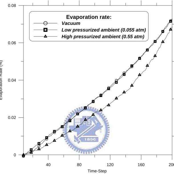
2.8.2 Evaporation rate... 29

2.8.3 Energy transfer process... 30

2.8.4 Surface tension... 30

2.9 Summary...32

Chapter 3 Parallel Cellular Molecular Dynamics (PCMD) Simulation Method .33 3.1 Reviews of parallel molecular dynamics method ...33

3.1.1 Atomic–decomposition algorithm... 33

3.1.2 Force–decomposition algorithm ... 34

3.1.3 Spatial–decomposition algorithm ... 34

3.2 Proposed PCMD method ...35

3.2.2 Repartitioning scheme ... 37

3.2.3 Decision policy for repartitioning... 39

3.2.4 Simulation conditions ... 41

3.2.5 Parallel performance ... 42

3.2.6 Summary... 44

Chapter 4 Simulation of argon droplet-droplet collision dynamics ...46

4.1 Simulation conditions ...46

4.1.1 Droplet formation... 47

4.1.2 Background gas formation... 47

4.1.2 Test conditions ... 48

4.2 Results and discussion ...49

4.2.1 Droplet-droplet collision under vacuum environment... 50

4.2.2 Droplet-droplet collision under low pressurized ambient... 53

4.2.3 Droplet-droplet collision under high pressurized ambient... 58

4.2.4. Data analysis ... 64

4.2.5 Distribution map of various regimes... 65

4 .3 Summary...66

Chapter 5 Concluding Remarks ...67

5.1 Summary...67

5.2 Recommendation for the future work ...68

References ...69

Tables...72

Figures...74

Autobiography...143

List of Tables

Table. 1 nondimensionalize ... 72 Table. 2 Simulation conditions for three different cases via PCMD code (condensed,

List of Figure

Fig. 1. 1 Terminology of possible droplet-droplet collision outcome, (a)

bounce, (b) coalescence, (c) disruption and (d) fragmentation... 74

Fig. 1. 2 Schematic of different droplet collision regimes as function of Weber number (We) and impact number (b)... 75

Fig. 2. 1 Cartesian frame... 76

Fig. 2. 2 Lennard-Jones (LJ) pairwise intermolecular potential ... 77

Fig. 2. 3 Water molecules i and j... 78

Fig. 2. 4 periodic boundary conditions ... 79

Fig. 2. 5 (a.)all pair, (b)cell link, and (c)Verlet list methods... 80

Fig. 2. 6 Verlet list... 81

Fig. 2. 7 Verlet +Cell link ... 82

Fig. 2. 8 Surface tension concept by Tabor [1991] ... 83

Fig.3. 1 Proposed flow chart for parallel molecular dynamics simulation using dynamic domain decomposition... 84

Fig. 3. 1 Evolution of domain decomposition for large problem size using 25 processors at start and final. (a) condensed state; (b) vaporized state; (c) supercritical state... 85

Fig.3.3 Distribution of the number of atoms in each processor as a function of simulation time steps (25 processors). (a) condensed state; (b) vaporized state; (c) supercritical state... 86

Fig.3.4 Parallel speedup as a function of the number of processors for three different test cases (condensed, vaporized and supercritical states). ... 87

Fig. 4. 1 Distribution map of various regimes under vacuum ambient... 88

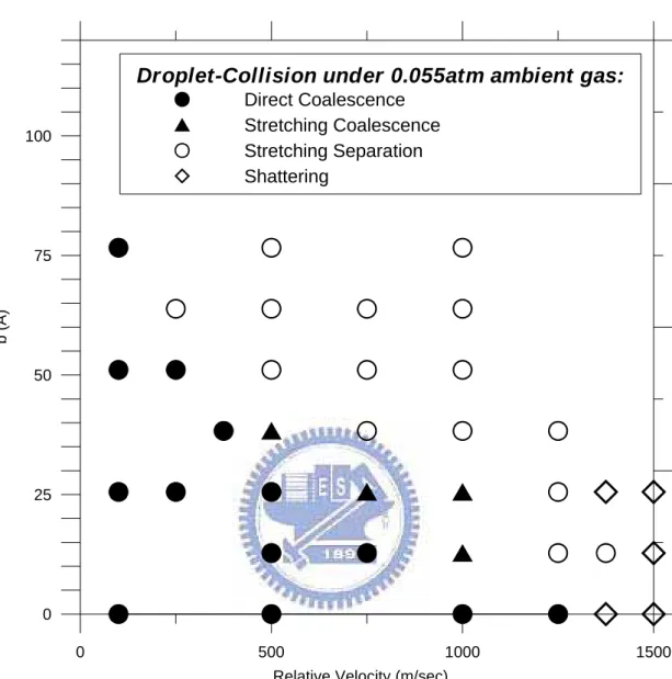
Fig. 4. 2 Distribution map of various regimes under low pressurized ambient (~0.055 atm). ... 89

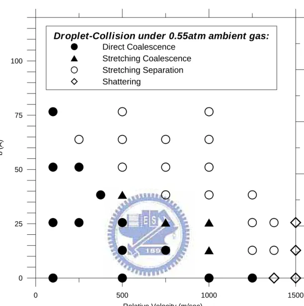
Fig. 4. 3 Distribution map of various regimes under high pressurized ambient (~0.55 atm). ... 90

Fig. 4.5 Head-on (b= 0) droplets pair collision initial setup, (a) y-z plane without vapor ambient, (b) x-z plane without vapor ambient, (c) y-z plane under vapor ambient, (d) x-z plane under vapor ambient ... 92

Fig. 4.6 Non-head-on (ex; b= 0.5) droplets pair collision initial setup, (a) x-y plane without vapor ambient, (b) x-y plane under vapor ambient... 93

Fig. 4.7 Snapshot of droplet pair collision under vacuum b=0 V=1250 m/s, at (a)10ps, (b)50ps, (c)75ps, (d)100ps, (e)125ps, (f)175ps... 94

Fig. 4.8 Snapshot of droplet pair collision under vacuum, b=0, V=1375 m/s, at (a)10ps, (b)40ps, (c)75ps, (d)150ps, (e)200ps, (f)300ps. ... 95

Fig. 4.9 Snapshot of droplet pair collision under vacuum, b=0, V=1500

m/s, at (a)10ps, (b)30ps, (c)75ps, (d)100ps, (e)175ps, (f)300ps. ... 96 Fig. 4.10 Snapshot of droplet pair collision under low pressurized

ambient (~0.055 atm), b=0, V=1250 m/s, at (a)10ps, (b)40ps, (c)75ps,

(d)100ps, (e)125ps, (f)200ps... 97 Fig. 4.11 Snapshot of droplet pair collision under low pressurized

ambient (~0.055 atm), b=0, V=1375 m/s, at (a)10ps, (b)40ps, (c)75ps,

(d)100ps, (e)150ps, (f)250ps... 98 Fig. 4.12 Snapshot of droplet pair collision under low vapor ambient, b=0, V=1500 m/s, at (a)10ps, (b)40ps, (c)60ps, (d)90ps, (e)150ps, (f)250ps.99 Fig. 4.13 Snapshot of droplet pair collision under high vapor ambient,

b=0, V=1250 m/s, at (a)10ps, (b)40ps, (c)75ps, (d)100ps, (e)125ps, (f)200ps... 100 Fig. 4.14 Snapshot of droplet pair collision under high vapor ambient,

b=0, V=1375 m/s, at (a)10ps, (b)40ps, (c)75ps, (d)100ps, (e)250ps, (f)325ps... 101 Fig. 4.15 Snapshot of droplet pair collision under high vapor ambient,

b=0, V=1500 m/s, at (a)10ps, (b)40ps, (c)60ps, (d)90ps, (e)150ps,

(f)250ps... 102 Fig. 4.2 Snapshot of droplet pair collision under vacuum, b=0.25, V=250

m/s, at (a)10ps, (b)50ps, (c)100ps, (d)200ps, (e)250ps, (f)375ps. This case is classified in Coalescence regime. ... 103 Fig. 4.3 Snapshot of droplet pair collision under vacuum, b=0.625,

V=1000 m/s, at (a)10ps, (b)40ps, (c)75ps, (d)100ps, (e)150ps, (f)250ps. This case is classified in Stretching Separation regime. ... 104 Fig. 4.4 Snapshot of droplet pair collision under vacuum b=0.25, V=1375

m/s, at (a)10ps, (b)40ps, (c)75ps, (d)100ps, (e)150ps, (f)250ps. This case is classified in Shattering regime... 105 Fig. 4.5 Snapshot of droplet pair collision under low pressurized ambient,

b=0.25, V=250 m/s, at (a)10ps, (b)50ps, (c)100ps, (d)200ps, (e)250ps, (f)375ps. This case is classified in Coalescence regime. ... 106 Fig. 4.20 Snapshot of droplet pair collision under low pressurized

ambient, b=0.25, V=750 m/s, at (a)10ps, (b)40ps, (c)75ps, (d)150ps,

(e)250ps, (f)500ps. This case is classified in Stretching Coalescence regime. ... 107 Fig. 4.21 Snapshot of droplet pair collision under low pressurized ambient,

b=0.625, V=1000m/s, at (a)10ps, (b)40ps, (c)75ps, (d)100ps, (e)150ps, (f)250ps. This case is classified in Stretching Separation regime... 108

Fig. 4.22 Snapshot of droplet pair collision under low pressurized

ambient, b=0. 25, V=1375m/s, at (a)10ps, (b)40ps, (c)75ps, (d)100ps,

(e)150ps, (f)250ps. This case is classified in Shattering regime. ... 109 Fig. 4.23 Snapshot of droplet pair collision under high pressurized

ambient, b=0.25, V=250 m/s, at (a)10ps, (b)50ps, (c)100ps, (d)200ps,

(e)250ps, (f)375ps. This case is classified in Coalescence regime. .... 110 Fig. 4.24 Snapshot of droplet pair collision under high pressurized

ambient, b=0.25, V=750 m/s, at (a)10ps, (b)40ps, (c)75ps, (d)150ps,

(e)250ps, (f)500ps. This case is classified in Stretching Coalescence regime. ...111 Fig. 4.25 Snapshot of droplet pair collision under high pressurized

ambient, b=0.625, V=1000m/s, at (a)10ps, (b)40ps, (c)75ps, (d)100ps,

(e)150ps, (f)250ps. This case is classified in Stretching Separation regime. ... 112 Fig. 4.26 Snapshot of droplet pair collision under high pressurized

ambient, b=0.25, V=1500m/s, at (a)10ps, (b)40ps, (c)75ps, (d)100ps,

(e)150ps, (f)250ps. This case is classified in Shattering regime. ... 113 Fig. 4.27 Snapshot of droplet pair collision under high pressurized

ambient, b=0, V=10 m/s, at (a)25ps, (b)250ps, (c)500ps, (d)750ps,

(e)1000ps, (f)1250ps. This case is classified in Bounce regime. ... 114 Fig. 4.28 Snapshot of droplet pair collision under high pressurized

ambient, b=0, V=30 m/s, at (a)25ps, (b)250ps, (c)500ps, (d)750ps,

(e)1000ps, (f)1250ps. This case is classified in Bounce regime. ... 115 Fig. 4.29 Snapshot of droplet pair collision under high pressurized

ambient (0.55 atm, T=324K ), b=0, V=10 m/s, at (a)25ps, (b)250ps,

(c)500ps, (d)750ps, (e)1000ps, (f)1200ps. This case is classified in

Bounce regime... 116

Fig. 4.30 Snapshot of droplet pair collision under high pressurized

ambient (0.55 atm, T=324K ), b=0, V=30 m/s, at (a)25ps, (b)250ps,

(c)500ps, (d)750ps, (e)1000ps, (f)1250ps. This case is classified in

Bounce regime... 117

Fig. 4.31 Snapshot of density contour and clusters size distribution under

vacuum, b=0, V=1250 m/s, at (a)25ps, (b)75ps, (b)150ps. This case is

classified in Stretching Coalescence regime. ... 118 Fig. 4.32 Snapshot of density contour and clusters size distribution under

low pressurized ambient, b=0, V=1250 m/s, at (a)25ps, (b)75ps,

(b)150ps. This case is classified in Stretching Coalescence regime. . 119 Fig. 4.33 Snapshot of density contour and clusters size distribution under

high pressurized ambient, b=0, V=1250 m/s, at (a)25ps, (b)75ps,

(b)150ps. This case is classified in Stretching Coalescence regime. . 120 Fig. 4.34 Snapshot of density contour and clusters size distribution under

vacuum, b=0, V=1500 m/s, at (a)25ps, (b)75ps, (b)150ps. This case is

classified in Shattering regime. ... 121 Fig. 4.35 Snapshot of density contour and clusters size distribution under

low pressurized ambient, b=0, V=1500 m/s, at (a)25ps, (b)75ps,

(b)150ps. This case is classified in Shattering regime. ... 122 Fig. 4.36 Snapshot of density contour and clusters size distribution under

high pressurized ambient, b=0, V=1500 m/s, at (a)25ps, (b)75ps,

(b)150ps. This case is classified in Shattering regime. ... 123 Fig. 4.37 Measurements of largest fragment of droplet pair collision under

vacuum, b=0.25, V=250 m/s, (a)Number of atoms, (b)Vibrational

temperature (k), (c)Rotational energy, (d)Angular momentum,

respectively. This case is classified in Coalescence regime... 124 Fig. 4.38 Measurements of largest fragment of droplet pair collision under

vacuum, b=0.625, V=1000 m/s, (a)Number of atoms, (b)Vibrational

temperature (k), (c)Rotational energy, (d)Angular momentum, respectively. This case is classified in Stretching Separation regime. ... 125 Fig. 4.39 Measurements of largest fragment of droplet pair collision under

vacuum, b=0.25, V=1375 m/s, (a)Number of atoms, (b)Vibrational

temperature (k), (c)Rotational energy, (d)Angular momentum,

respectively. This case is classified in Shattering regime. ... 126 Fig. 4.40 Measurements of largest fragment of droplet pair collision under

low pressurized ambient, b=0.25, V=250 m/s, (a)Number of atoms,

(b)Vibrational temperature (k), (c)Rotational energy, (d)Angular

momentum, respectively. This case is classified in Coalescence regime. ... 127 Fig. 4.41 Measurements of largest fragment of droplet pair collision under

low pressurized ambient, b=0.25, V=750 m/s, (a)Number of atoms,

(b)Vibrational temperature (k), (c)Rotational energy, (d)Angular momentum, respectively. This case is classified in Stretching

Coalescence regime... 128

Fig. 4.42 Measurements of largest fragment of droplet pair collision under

low pressurized ambient, b=0.625, V=1000m/s, (a)Number of atoms,

(b)Vibrational temperature (k), (c)Rotational energy, (d)Angular momentum, respectively. This case is classified in Stretching

Separation regime... 129

Fig. 4.43 Measurements of largest fragment of droplet pair collision under

low pressurized ambient, b=0.25, V=1375m/s, (a)Number of atoms,

(b)Vibrational temperature, (c)Rotational energy, (d)Angular momentum, respectively. This case is classified in Shattering regime. ... 130 Fig. 4.44 Measurements of largest fragment of droplet pair collision under

high pressurized ambient, b=0.25, V=250 m/s, (a)Number of atoms,

(b)Vibrational temperature (k), (c)Rotational energy, (d)Angular

momentum, respectively. This case is classified in Coalescence regime. ... 131 Fig. 4.45 Measurements of largest fragment of droplet pair collision under

high pressurized ambient, b=0.25, V=750 m/s, (a)Number of atoms,

(b)Vibrational temperature (k), (c)Rotational energy, (d)Angular momentum, respectively. This case is classified in Stretching

Coalescence regime... 132

Fig. 4.46 Measurements of largest fragment of droplet pair collision under

high pressurized ambient, b=0.625, V=1000m/s, (a)Number of atoms,

(b)Vibrational temperature (k), (c)Rotational energy, (d)Angular momentum, respectively. This case is classified in Stretching

Separation regime... 133

Fig. 4.47 Measurements of largest fragment of droplet pair collision under

high pressurized ambient, b=0.25, V=1500m/s, (a)Number of atoms,

(b)Vibrational temperature, (c)Rotational energy, (d)Angular

momentum, respectively. This case is classified in Shattering regime. ... 134 Fig. 4.48 Measurements of largest fragment of droplet pair collision under

high pressurized ambient, b=0, V=30m/s, (a)Number of atoms,

(b)Vibrational temperature (k), (c)Rotational energy, (d)Angular

momentum, respectively. This case is classified in Bouncing regime.135 Fig. 4.49 The atoms distributions in X direction of bounce case under high

pressurized ambient, b=0, V=10 m/sec. ... 136

Fig. 4.50 The atoms distributions in X direction of bounce case under high

pressurized ambient, b=0, V=30 m/sec.. ... 137

Fig. 4.51 The atoms distributions in X direction of bounce case under high

pressurized ambient (0.55 atm, T=324 K), b=0, V=10 m/sec... 138

Fig. 4.52 The atoms distributions in X direction of bounce case under high

pressurized ambient(0.55 atm, T=324 K), b=0, V=30 m/sec... 139

under low pressurized ambient (0.055 atm, T=216 K), b=0.25, V=750

m/sec.. ... 140 Fig. 4.54 The variation of surface tensions distributions of separation case

under low pressurized ambient (0.055 atm, T=216 K), b=0.625,

V=1000 m/sec.. ... 141 Fig. 4.55 The variation of surface tensions distributions of bouncing case

under low pressurized ambient (0.055 atm, T=216 K), b=0, V=30

Nomenclature

ρ _{: density} τ : surface tension B k _{: Boltzmann’s constant} i rot

v _{, : angular velocities of i atom} D : diameter of droplet

r : radius of droplet

i

r _{: the position vector of moleculei}

i

F : the force vector of moleculei

i

p : the momentum vector of moleculei

V _{: relative velocity} U _{: potential} N _{: number of density} n _{: number of atoms} T :temperature vib T : vibrational temperature E : energy rot E : rotational energy

Chapter 1 Introduction

1.1 Motivation

1.1.1 Droplet collision dynamics

Droplet collision dynamics plays a key role in various technologies such as, spray combustion, ink-jet printing, rain drop formation, insecticide spraying, nuclear fusion, surface coating, and solidification, among others. In addition, collision between two droplets becomes the most frequent event in theses applications. Thus, understanding of the fundamental collision dynamics between two droplets becomes crucial in optimizing these applications. Depending upon the size of the droplets, descriptions of the collision dynamics can be generally classified into continuum-scale and atomic-scale, which are described next.

1.1.2 Continuum-scale description

Process of droplet collision itself is very complicated, while it follows conservation of energy, conservation of momentum, and conservation of angular momentum. In a collision, the droplet loses kinetic energy as the droplet strains and deforms. The strains lead to viscous dissipation, accounting for some conversion of mechanical energy to heat. More importantly, the droplet surface increases as the original droplet breakdowns into smaller ones and surface energy increases accordingly. The surface energy can be viewed as a potential energy and conversion

of kinetic energy to surface energy can be viewed as a conservative process. The increase of surface energy during the early part of a collision results in recoiling and rebounding later through the conversion of surface energy back to kinetic energy. The momentum balance occurs through a force imposed on the droplet by the other droplet in a collision as the droplet loses inertia and possibly rebounds in the other direction. For collisions between droplets that are not head-on, we can expect that conservation of angular momentum acts through a torque imposed during collision, which makes the colliding droplet rotating.

Collision dynamics between two droplets had attracted much attention in continuum scale, while it had not been well studied in the atomic scale. In this thesis, we intend to fill in this gap to provide more detailed inside about droplet collision dynamics in the nanoscale regime.

1.1.2 Atomic-scale description

In the atomic scale, continuum-scale description may fail since continuum assumption may breakdown due to very large gradient of properties caused by very small length scale. Droplet collision in this scale requires different approaches as those in continuum scale. One of the most often adopted approaches is to utilize molecular dynamics (MD) simulation to understand these non-equilibrium phenomena. Also it is interesting and possibly important in the present

nanotechnology to understand if the collision dynamics bwteen two nanoscale droplets share the same physical pictures as those in the continuum scale? In addition, understanding of the atomic-scale collision dynamics may further improve the understanding of the continuum-scale collision dynamics.

1.2 Background

1.2.1 Droplet collision dynamics

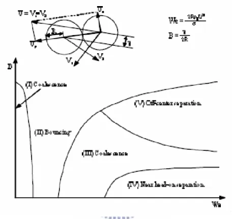
In this thesis, we focus on the collision dynamics between two nanoscale droplets. Based on the understanding in the continuum scale, droplet collision can be generally classified into different types of collision depending on some critical parameters, as shown in Fig. 1.1. These different types of collision process are introduced next.

1.2.1.1 Droplet bouncing

Droplets bouncing occurs if the surfaces of the droplets do not make contact due to the presence of a thin intervening gas film in between. In this case the droplet’s surfaces undergo a flattening deformation, but the surfaces do not make contact since the kinetic energy of collision (CKE), is insufficient to expel the intervening layer of gas.

1.2.1.2 Droplet coalescence

Droplet coalescence, in which an integrated post-collision droplet is formed whose mass is equal to the sum of the mass of the pre-collision droplets, follows after

the droplet contacts. The colliding droplets coalesce when the air film thickness reaches a critical value (~102 _{Å, Mackay et. al.[1963]). The droplets may coalescence}

temporarily or permanently, depending on the CKE and impact parameter (b).

1.2.1.3 Disruption and fragmentation

Temporary coalescence occurs when the CKE exceeds the value for stable coalescence and eventually results in either disruption or fragmentation. Disruption is that case when the collision product separates into the same number of droplets which exists prior to the collision. A collision resulting in bouncing may be difficult to distinguish from the case when the temporary coalescence followed by disruption results in two droplets with masses equal to the pre-collision droplet masses. As for fragmentation, the coalesced droplet undergoes catastrophic break-up into numerous small droplets.

1.2.2 Crucial parameters in describing droplet collision dynamics 1.2.2.1 Continuum-scale description

In the continuum scale, it is convenient to characterize the collision process in terms of the Webber number (We), the impact parameter (b) and Kinetic energy of collision (CKE). Schematic diagram showing different droplet collision regimes as functions of Weber number (We) and impact parameter (b) is shown in Fig. 1.3. Physical meaning of the above these important parameters are described in the following for completeness.

1.2.1.1.1 Weber number (We)

The Webber number is the ratio of the inertial force to the surface force and is defined as: τ ρ 2 / s D V We= (1.1)

where ρ is the droplet density, D is the diameter of the smaller droplet and _s τ is

the surface tension of the droplet fluid.

1.2.1.1.2 Impact parameter (b)

The impact parameter (b), (Fig. 1.3), is defined as the distance from the center of one droplet to the relative velocity vector placed on the center of the other droplet.

1.2.1.1.3 Kinetic energy of collision (C.K.E)

The kinetic energy of collision (CKE) of the droplet pair with the same droplet fluid is given by (Low and List [1982]):

(

)

2 3 3 3 3 12 _{L S} L S S L _{V V} D D D D CKE _⎟⎟ − ⎠ ⎞ ⎜⎜ ⎝ ⎛ + = ρπ (1.2)

The above can be rewritten as:

(

)

2 3 3 1 12 L S L _{V V} R D CKE _⎟⎟ − ⎠ ⎞ ⎜⎜ ⎝ ⎛ + = ρπ (1.3)

where R is the droplet size ratio r / . Where r_L r_S L and rS is radius of droplet large

and droplet small, respectively.

1.2.2.2 Atomic-scale description

In the atomic scale, characterizing the droplet collision using the above-mentioned parameters may be misleading. Alternative way of description

becomes necessary. Among these, description using the concept of N-body dynamics Jellinek and Li [1989] may become a reasonable way to highlight the underlying physics of the collision process. In what follows, we briefly introduce the concept of N-body dynamics in section 2.8.5.

1.3 Literature reviews

1.3.1 Droplet growth

Hu, et al. [1998], propose the stochastic growth of cloud droplet distributions due to collection processes is studied using a detailed microphysical parcel model. The evolution of rainwater content (L-R) and the radar reflectivity factor (Z) are plotted in order to trace the progress of transfer of cloud water into rainwater and determine the importance of droplet collection in different size ranges. The results indicate that the van der Waals forces are effective in enhancing droplet collision when the droplets are small and the distributions are narrow.

1.3.2 Droplet-droplet collision

Ashgriz and Poo [1990] carried out collision experiments with water drops in the micrometer to millimeter size range. Two drop streams collided with relative velocities of 1–20 m/s, and single collisions were followed with high-speed video recording. Two different types of separating collisions were identified, reflexive and stretching separating, and they determined the boundaries between these processes

and coalescence. Reflexive separation was found for near head-on collisions with high velocity while stretching separation occurred for large impact parameter.

Panand Law [2004], presented a dynamics of head-on collision between two identical droplets was experimentally and computationally investigated, with particular emphasis on the transitions from merging to bouncing to merging again as the collision Weber number increased.

Later, Pan and Law [2005] extend the research to a head-on collision of a droplet onto a liquid layer of the same material, sitting on a solid surface. Both experimental and computational methods were applied to illuminate the transition from bouncing of the droplet to its absorption by the film for given droplet Weber number, We, and the film thickness scaled by the droplet radius, Hf.

1.3.3 Simulation methods for droplet collision dynamics

The simulation methods for droplet collision dynamic can be classified into two major groups, depending on the size scale of simulation system. as the

continuum-scale and atomic-scale methods.

1.3.3.1 Continuum-scale simulation methods 1.3.3.1.1 Navier-Stokes equation method

Harlow and Shannon [1967] were the first to simulate droplet impact on the solid surface. They used a “marker-and-cell” (MAC) finite-difference method to solve the fluid mass and momentum conservation equations. Tsurutani et al. [1990] enhanced

the MAC model to include surface tension and viscosity effects, and also considered heat transfer from a hot surface to a cold liquid droplet as it spread on the surface. Trapaga and Szekely [1991] used the “volume of fluid” (VOF) method, to study impact of molten particles in a thermal spray process. Liu et al. employed another VOF based code, to simulate molten metal droplet impact. Zhao et al. [1996] formulated a finite-element model of droplets deposited on solid surfaces. Adaptive-grid finite element methods were used first by Fukai et al. [1995] to simulate water droplet impact, and later by e.g., [Bertagnolli et al., 1997], [Waldvogel and Poulikakos, 1997] to study thermal spraying of molten ceramic particles.

Bussmann et al. [1999] publish a description of a three-dimensional, fine-difference, fixed-grid Eulerian model the developed, to simulate water droplets falling with low velocity (~1m/s), onto either an inclined plane or the edge of a step. Pasandideh-Fard et al. [2002] extended the 3-dimensional model of Bussmann’s model to include heat transfer and solidification. In addition, they also accommodate the presence of an irregular moving solidification front within the computational grid.

1.3.3.1.2 Lattice Boltzmann methods

Lattice Boltzmann method [Succi, 2001] excels in modeling flow problems involving multiphase materials and complicated geometry. It is highly suitable to model the droplet collision dynamics. For example, Inamuro, et al. [2004] presented a

applied the method to the simulations of binary droplet collisions for various Weber numbers and impact parameters. They simulated the there exist other types of binary droplet collisions under certain conditions, bouncing collision for low Weber numbers and shattering collision (Disruption or fragmentation) for high Weber numbers and discussed the mixing processes in different conditions.

1.3.3.2 Atomic-scale simulation methods 1.3.3.2.1 Molecular dynamics under vacuum

Greenspan and Heath [1991] studied the collision dynamics of nanometer-sized particles. They carried out classical trajectory calculations of collisions between water clusters with a size of 2051 monomers. The individual molecules were modeled as single mass particles and the molecule–molecule interaction was described by a Lennard–Jones potential. Different modes that the colliding system could obtain were identified and compared with observations made for colliding large drops.

Gay and Berne [1986]studied head-on collisions between clusters where the atom–atom interaction was described by a L-J pair potential. They varied the cluster size ~19–135 atoms/cluster in the same temperature, and relative velocity and found that the collisions were accompanied by internal heating and that the clusters coalesced.

Svanberg et al. [1997] performed MD calculations of collision between Ar1000

parameter (0-4 nm) on energy transfer and dynamical behavior.

Later, Svanberg et al. [1998] increased the complexity of the system and studied the droplet collision dynamics of liquid-like water clusters with an internal temperature of 300K. Collisions between (H2O)n (n=125, 1000), and investigated the

effects of cluster velocity and impact parameter on the outcome of the collisions. Blaisten–Barojas and Zachariah [1992] studied Si15–Si15 collisions at a temperature

of about 2000K using molecular dynamics. Chen et al. [1993] carried out molecular dynamics simulations of Au55-Au55 collisions using an embedded atom method

potential. Collisions with clusters initially at 0 or 300K were studied, and all collisions resulted in cluster aggregation with significant inelastic deformation of the original clusters.

1.3.3.2.2 Molecular dynamics with ambient gas

Murad and Law [1999] presented a molecular dynamic simulation with L-J potential for droplet–droplet collision with ambient gas. Bouncing between droplets was only found within a narrow band of state conditions collision, which is mainly attributed to the existence of background gas. However, not much parametric study has been conducted to further understand the effects of the ambient pressure..

Based on the reviews in the above, only preliminary studies have been done in the simulation of nanoscale droplet-droplet collision. Understanding of the droplet

technology. Thus, MD simulation will be used to study the physics of the droplet-droplet collision dynamics in the nanocale regime.

1.4 Objectives of the thesis

The specific objectives of the thesis are summaried as follows:

1. To develop and verify a parallelized cellular molecular dynamics (PCMD) simulation code, which takes advantage of the link-cell data structure, using dynamic domain decomposition.

2. To study and explain the droplet-droplet collision dynamics in the nanoscale regime using the developed PCMD code under vacuum and pressured environment.

1.5 Organization of the thesis

In this thesis, Chapter 2 describes the classical MD simulation method and some specific ways of MD data analysis used in the present thesis. Chapter 3 describes the past efforts in parallel MD method, the proposed PCMD method in detail and its resulting parallel performance. Chapter 4 describes the simulation of droplet-droplet collision dynamics using the PCMD code. Finally, Chapter 5 describes the concluding remarks with some recommendation for the future study.

Chapter 2 Molecular Dynamics Simulation

2.1 Basic molecular dynamics simulation

Molecular dynamics (MD) has been widely used to simulate properties of liquids, solids, and molecules in several research disciplines. It is an important approach to understand microscopic character of nature. MD is derived form a new concept called, phase trajectory. We computed the trajectories of molecules using classical Newtonian mechanics and we described features of the molecule trajectory in classical nonlinear dynamics. And obtain properties by analyze the trajectory with kinetic theory, statistical mechanics, and sampling theory. In addition, periodic boundary conditions and conservation principles are used to hold accuracy of MD simulation. Combined these tools form the foundation of molecular dynamics.

Newtonian Second Law:

2 2 2 t d r d m r m F i i i = &&= (2.1)

where ri is the position vector of molecule i as shown in Fig. 2.1

Since Newton’s second law is time independent or equivalently

2 2 2 t d r d m r m F i i

i = &&= is invariant under time translations. Consequently, we expect there

to be some function of the positions and velocities whose value is constant in time; this function is called the Hamiltonian,

const p

r

H₍ N_, N_{)= (2.2)}

where p_i =mr_&i is the momentum of molecule i.

For an isolated system, total energy E is conserved, where E is equal to the sum of kinetic energy and potential energy. Thus, for an isolated system, we identify total energy as the Hamiltonian; then for N spherical molecules, H can be written as

∑

+ = = i N i N N _{p U r E} m p r H ( ) 2 1 ) , ( 2 _(2.3)

where )_U(_rN _{results from the intermolecular interactions.}

First consider the total time derivative of the general Hamiltonian (2.2),

∑

∑

⋅ +∂_∂ ∂ ∂ + ⋅ ∂ ∂ = i i i i i i t H r r H p p H dt dH & & (2.4)

If, as is (2.3), H has no explicit time dependence, then the last term on the RHS of (2.4) vanishes and we are left with, due to H=const,

∑

∑

⋅ = ∂ ∂ + ⋅ ∂ ∂ = i i i i i i r r H p p H dt dH 0 & & (2.5)

If Hamiltonian is expressed as (2.6), then

∑

∑

⋅ = ∂ ∂ + ⋅ = i i i i i i r r U p p m dt dH 0 1 & & (2.6)

On comparing (2.5) and (2.6), we find for each molecule i,

i i i r m p p H & = = ∂ ∂ (2.7)

and i i r U r H ∂ ∂ = ∂ ∂ (2.8)

Substituting (2.7) into (2.5) gives

∑

∑

⋅ = ∂ ∂ + ⋅ i i i i i i r r U p

r_{& & &} 0 (2.9)

or ( )⋅ =0 ∂ ∂ +

∑

i i i i r r H p_{& &} (2.10)

Since the velocities are all independent of one another, (2.10) can be satisfied only, for each molecule i, we have

i i p r H & − = ∂ ∂ (2.11)

Eq.(2.7) and (2.11) are Hamilton’s equation of motion. For a system of N particles, (2.7) and (2.11) represent 6N first-order differential equations that are equivalent to Newton’s 3N second-order differential equations (2.1).

In the Newtonian view, motion is a response to an applied force. However, in the Hamiltonian view, motion occurs in such a way as to preserve the Hamiltonian function, where the force does not appear explicitly.

For an isolated system, the particles move in accordance with Newton’s second law, tracing our trajectories that can be represented by time-dependent position vectors ri(t). Similarly, we also have time-dependent momentum pi(t).

6N-dimensional hyperspace. Such a space, called phase space, is composed of two parts: a 3N-dimensional configuration space, in which the coordinates are the components of position vectors ri(t), and a 3N-dimensional momentum space (or

velocity space), in which the coordinates are the components of the momentum vectors pi(t). As time evolves, the points defined by positions and momentum in the

6N phase space moves, describing a trajectory in phase space.

2.2 Potential model

We can say that the potential model is the role of molecular dynamic simulation. As you want approach the different realistic material in simulation, you have to change the potential model. Because the force on an atom in simulation is due to interaction with surrounding neighbors. And the force is derived from potential. To creative a potential model you must to do a lot of abstruse computations in Quantum Chemistry. Fortunate, there are a lot accurate potential model had been devised by chemists and physicists, today. There are some potential models will be introduce as follow.

2.2.1 Lennard-Jones potential

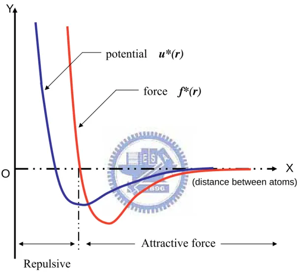
The potential first introduced by J.E. Lennard-Jones [1924]. The pair-wise intermolecular potential form as follow:

_{ij c} ij ij ij r r r r r U( )=4_ε[(σ )12 −(σ)6], ≤ _(2.12)

where r_ij =r_i−r_j and is shown in Fig.2.2. The parameter ε presents the strength of the interaction and σ defines a length scale. This potential repels at close range, then attracts, and is eventually cut off at some limiting separation rc. While the

strongly repulsive core arising from the nonbonded overlap between the electron clouds has a rather arbitrary form (other powers and functional form are sometimes used), the attractive tail actually represents van der Waals interaction due to electron correlations. Most importantly, this L-J potential assumes the interactions involve individual pairs of atoms: each pair is treated independently, with other atoms in the neighborhood having no effect on the force between them.

Force resulting from LJ potential is written as ) (r U f =−∇ (2.13) or _ij ij ij ij r r r f ( ) ] 2 1 ) )[( 48 ( 14 8 2 σ σ σ ε ₋ = (2.14)

provided r_ij ≤ , zero otherwise and is shown in Fig. 3.2. As r increases towards r_c rc the force drops to zero, so that there is no discontinuity at rc; f and higher

derivatives are discontinuous.

In general, we would like to express these equations used in MD in dimensionless format. There are several reasons for doing this, not the least being the ability to work with numerical values not far from unity, instead of the extremely

values normally associated with the atomic scale. Another benefits of using dimensionless units is that the equations of motion are simplified because some, if not all, of the parameters defining the model are absorbed into the units. Finally, using such dimensionless units lies in the fact that general notion of scaling can be applied to whole class of problems. Of course, from practical viewpoint, the switch to such units removes any risk of encountering values lying outside the range that is representable by the computer hardware. Units used to nondimensionalize the related MD equations are listed in Table 1 for reference.

2.2.2 Water potential

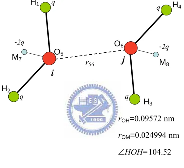
The biggest difference between the water potential and the L-J potential is the polar and structure of molecule of water potential. For water molecule i and j shown in Fig.2.3, the effective pair potential u

( )

r_ij is actually a function of the distances among the two sets of atoms and point changes, That is,

( )

r f

(

r13,r14,r16,r18,r23,r24,r26,r28,r35,r37,r45,r47,r56,r78

)

u _ij = (2.15)

where the indices 1, 2, 3, 4, 5, 6, 7 and 8 denote the site of atoms or point charges H1, H2, H3, H4, O5, O6, M7 and M8.

On the other hand, the rotational motion of water molecule i is simulated based on the angular momentum equation of motion,

dt dH

M i

where Mi and Hi are the moment vector and angular momentum vector acting on

the molecule i.

2.3 Initial conditions

1. A minimum requirement for the MD simulation to be valid is that the results of a simulation of adequate duration are insensitive to the initial state, so any convenient initial state is allowed.

2. A particular simple but practical choice is to start the with the particles at the sites of some regular lattice, e.g., the square or simple cubic lattice, and spaced to give the desired density.

3. The velocities are assigned random directions and a fixed magnitude based on temperature.

4. The speed of equilibration to a state in which there is no memory of this arbitrarily selected initial configuration is normally quite rapid, so that more careful attempts at the constructing a ‘typical” state are of little benefit.

2.3.1 Initial coordinates

For FCC lattice, there are four atoms per unit cell, and the system is centered at the origin.

2.3.2 Initial velocities

The velocity magnitude is fixed, each velocity vector is assigned a random direction, and the velocities are then adjusted to ensure that the center of mass is at rest.

2.3.3 Initialization of integration variables

For leapfrog method, if the users do not care the minor difference between t=0 and t=∆t/2 in setting the initial velocities, then there is no further work required. If the difference is not to be overlooked, a single interaction computation is all that is required.

2.4 Boundary condition

2.4.1 Periodic boundary Condition

Unless the purpose of the MD simulation is to capture the physics near real walls, a problem that is actually of considerable importance, walls are better eliminated by using periodic boundary conditions (PBC). Physical meaning of periodic boundary conditions is shown in Fig. 2.4. The introduction of PBC is equivalent to considering an infinite space-filling array of identical copies of simulation region.

There are some consequences of this PBC:

face immediately reenters the region through the opposite face.

2. A wraparound effect needs to be considered. Particles lying within a distance rc of a boundary interact with particles in an adjacent copy of the

system, or, equivalently, with particles near the opposite boundary.

3. This wraparound effect of the PBC must be taken into account in both the

integration of the equations of motion and the interaction computations.

(checking the coordinates of particles if they move outside the region.) 4. Periodic boundary conditions are most easily handled if the region is

rectangular in two dimensions, or a rectangular prism in three dimensions. This is not an essential requirement, and any space-filling convex region can be used, although the boundary computation is not as easy as those in rectangular one. The motivation to choose alternative region shapes is to

enlarge the volume to surface ratio, thus increase the maximum distance

between particles before periodic ambiguity appears.

5. Using PBC will restrict the interaction range to no more than half the smallest region dimension.

6. Even with PBC, finite-size effects are still present. So how big the simulation region should be? It depends on what kind of system and the properties of the interest. As a minimum requirement, the size should

exceed the range of any significant correlations. Only detailed numerical experiments can hope to resolve this question.

2.4.2 Wall boundary conditions

When we simulate some problems, we would like to keep the wall isothermal. For the purpose, we define a correction layer on wall ,and there are two ways to modify correction layer on wall ; one is Rescaling method, the other is Langevin method.

2.4.2.1 Rescaling method

Rescaling method keep wall isothermal by modify total kinetic energy .In microcosmic size, temperature is related to kinetic energy, when we set the temperature of correction layer ,it means to set the average kinetic energy of atoms on the correction layer, so we must keep the kinetic energy fixed. (Eq. 2.17), so we have a reference valve. Then, use Eq.2.18 we compute the total kinetic energy of atoms. Finally, we start rescaling by using Eq.2.19 to make the total kinetic energy in the correction layer is the same as reference value which we computed in Eq.2.18

d B kd Nk T E 2 3 = (2.17) a B N i old i Ka m V Nk T E 2 3 2 1 1 2 = =

∑

= (2.18) a d i ka kd old i new i T T V E E V V = ⋅ = ∗ (2.19) where

kB : Boltzmann constant kd

E : the total kinetic energy define byT _d

ka

E : the total kinetic energy of atoms in the correction layer

d

T : the boundary temperature which we need

a

T : the average temperature of atoms in the correction layer before modification

old i

V : the velocity of atom in the correction layer before modification

new i

V : the velocity of atom in the correction layer r after modification

2.4.2.2 Langevin method

Langevin method keep thermal boundary isothermal by modifying equations of motion as below ) (t R v m U v m_i&i =−∇ − _iβ_{i i} + (2.20) where mi :mass of atom vi : atom velocity i β :Damping constant

R(t): Random Force ,which average valve is 0

2-5 Force computations

2.5.1 All pairs method

It is the simplest one to implement, but extremely inefficient when the interaction range rc is relatively small compared with the linear size of simulation region. In this

computational time grows as O(N2_{), where N is the number of particles. This}

constraint rules out the method for all but the smaller values of N. Two other techniques, including cell-link and Verlet list, to reduce the grow rate O(N2_{) are}

introduced next in turn.

2.5.2 Cutoff distance method 2.5.2.1 Cell-link

Basic idea of this method is to divide the simulation region into a lattice of small cells, and that the cell width exceeds rc. If particles are assigned to cells based on their

instantaneous positions, then it is obvious that interactions are only possible between particles that are either in the same cell or in immediately adjacent cells. Because of symmetry only half the neighboring cells need to be considered. For example, a total of 14 neighboring cells must be examined in three dimensions (include the cell itself). In addition, the wraparound effects can be readily incorporated into the scheme. In general, the region size must be at least 4 rc for this method to be useful.

There are several ways of implementing this cell-link list method to connect the relation between particles and cells. In the current demonstration code, it utilizes concept of the pointers for particles and cells. Each cell stores a particle number, which may be zero or nonzero. Nonzero value represents a true particle number, while the zero value represents either the last atom in the cell or an empty cell. In addition,

only one array cell List is used to represent the particles and cells. The obvious advantage of doing this is we know exactly the size of this array in advance if periodic boundary conditions are used. Of course, there are several other methods to implement this idea of cell-link list technique. Ideas depicting in the above can be clearly illustrated as Fig. 2.5:

2.5.2.2 Verlet list

A list of all particle pairs with separation rmax > rc is maintained and updated

every say 10 or 20 time steps. rmax is chosen large enough that it is unlikely that a

particle pair not in the list will come closer than rc before the list is updated. It is also

possible to decide automatically when the neighbor list needs to be updated. When the list is created, a vector for each particle is set to zero. At each time step, the vector is incremented by the particle displacement. For example, see the Fig. 2.6.

2.5.2.2 Cell link + Verlet list

we could combine cell link method and Verlet list method, see Fig. 2.7 ;by this way ,it could promote the performance of the simulation.

2.6 Equation of motion

2.6.1 Leap-Frog method

that are accurate to third order in ∆t. However, it tends to be considerably better than

the higher-order methods from the viewpoint of energy conservation. In addition, their storage requirements are also minimal.

The derivation of the Verlet formula follow simmediately from the Taylor expansion of the coordinate variable – typically x(t)

) ( ) ( ) 2 / ( ) ( ) ( ) (_{t h x t hx t h}2 _{x t O h}3 x + = + _& + _&& + (2.21) where t is the current time , and h≡∆t . Here, x& is the velocity component, (t) and )x&& the acceleration –or force f(t) in reduced MD units. Note that although (t

) (t

x&& has been expressed as a function of t, it is actually a known function – via the

force law – of the coordinates at time t. After rearrange Eq.2.21, we obtain ) ( ) ( ) ( ) ( 2 ) (_{t h x t x t h h}2_{x t O h}4 x + = − − + _&& + (2.22) The truncation error is of order _O(_h4)_{because the h term cancel. A possible} 3

disadvantage of Eq. 2.22 is that at low machine precision the _{h term multiplying the} 2

acceleration may prove a source of inaccuracy. The velocity is not directly involved in the solution, but if required it can be obtained from

) ( 2 / )] ( ) ( [ ) (_{t x t h x t h h O h}2 x_& = + − − + (2.23) with higher-order expression based on values from earlier time steps available if needed, though rarely used.

) ( )] ( ) 2 / ( ) ( [ ) ( ) (_{t h x t h x t h x t O h}3 x + = + _& + _&& + (2.24) The term multiplying h is just x&(t+h/2), so Eq.2.24 becomes 2.26 below. The leapfrog integration formulate are then

) ( ) 2 / ( ) 2 / (t h x t h hx t

x& + = & − + && (2.25) ) 2 / ( ) ( ) (t h x t hx t h x + = + & + (2.26) The fact that coordinates and velocities are evaluated at different times dose not present a problem; if an estimate for x& is required there is a simple connection (t) that can be expressed in either of two ways:

) ( ) 2 / ( ) 2 / ( ) (t x t h h x t

x& = & m ± && (2.27) The initial conditions can be handled in a similar manner, although a minor inaccuracy in describing the starting state, namely, the distinction between x&(0) andx&(h/2), is often ignored.

2.6.2 Gear’s predictor method

Predictor-corrector algorithms commonly used in molecular dynamics are often taken from the collection of methods devised by Gear. Predict molecular position ri a

time t+∆t using a fifth-order Taylor series based on positions and their derivatives at time t: ! 5 ) ( ! 4 ) ( ) ( ! 3 ) ( ) ( ! 2 ) ( ) ( ) ( ) ( ) ( 5 ) ( 4 ) ( 3 ) ( 2 _t r t t r t t r t t r t t r t r t t

! 4 ) ( ! 3 ) ( ) ( ! 2 ) ( ) ( ) ( ) ( ) ( 4 ) ( 3 ) ( 2 ) ( t r t t r t t r t t r t t r t t

r_& +∆ = _&i ∆ + _&&i ∆ + _iiii ∆ + _iiv ∆ + _iv ∆ (2.29)

! 3 ) ( ! 2 ) ( ) ( ) ( ) ( ) ( 3 ) ( 2 ) ( ) ( t r t t r t t r t r t t

r_&& +∆ = _&&i + _iiii ∆ + _iiv ∆ + _iv ∆ (2.30)

! 2 ) ( ) ( ) ( ) ( 2 ) ( ) ( ) ( ) ( _{t t r t r t t r} t riii _{+∆ = i}iii _{+ i}iv _{∆ + i}v ∆ _(2.31) t r t r t t r(iv)_{( +∆ )= i}(iv)_{( )+ i}(v)_{∆ (2.32)} ) ( ) ( ( ) ) ( _{t t r t} rv _{+∆ = i}v _(2.33)

[

r(t t) r (t t)

]

r_i = _i +∆ − _iP +∆

∆&& && &&

(2.34) In Gear’s algorithms for second-order differential equations, this difference term is used to correct all predicted positions and their derivatives; thus,

2 0 R r r_i = _iP+α ∆

(2.35) 2 1 R t r t r&_i∆ = &_iP∆ +α ∆

(2.36) 2 ! 2 ) ( ! 2 ) ( 2 2 2 R t r t r P i i ∆ ₌ && ∆ ₊α _∆ &&

_(2.37) 2 ! 3 ) ( ! 3 ) ( 3 3 ) ( 3 ) ( R t r t r iii P i iii i ∆ ₌ ∆ ₊α _∆

_(2.38) 2 ! 4 ) ( ! 4 ) ( 4 4 ) ( 4 ) ( R t r t r ivP i iv i ∆ ₌ ∆ ₊α _∆

_(2.39) 2 ! 5 ) ( ! 5 ) ( 5 5 ) ( 5 ) ( R t r t r v P i v i ∆ ₌ ∆ ₊α _∆

_(2.40) where ! 2 ) ( 2 2 t r R ₌ ∆i ∆ ∆ &&

(2.41)

α

0

=3/16, α

1

=251/360,α

2

=1, α

3

=11/18, α

4

=1/6, α

5

=1/60

2.7 Thermodynamic properties

Measurements of thermodynamic equilibrium properties can be considered as exercises in numerical statistical mechanics. MD simulation provides an alternative to

Monte Carlo (MC) simulation, and if no further information is required about the system, computational efficiency alone should determine the choice of simulation technique.

2.7.1 Absolute temperature

For an isolated system the total internal energy E is just the Hamiltonian ,which divides into a Kinetic part E and a configurational part _k U . _c

c k U E E= + (2.42) dr r r g r u N U_c 2 0 ( ) ( ) 2

∫

∞ = πρ (2.43) The average Kinetic energy is proportional to the absolute temperature:

NKT E_k 2 3 >= < (2.44) by Eq.2.44 so we could get the absolute temperature

Estimation of Cv: > < = 2 2 E T k N C B a v δ (2.45)

where _<δE2 _>=<E2 _{>−<E >}2 _{. However, this is inappropriate for the}

microcanonical (NVE) MD simulation since E=constant. Instead, it can be shown that, using the variance of Ek or Eu,

1 2 2 ) ) ( 3 2 1 ( 2 3 _{− < >} − = _k B a B v E T k N k C δ (2.46) 2.7.2 Pressure