以模糊推論系統與細胞自動機方法探討混合車流環境下機車行進行為

全文

(1)國立交通大學交通運輸研究所博士論文 No. 41. 以模糊推論系統與細胞自動機方法探討混合車流環境下機車行進行為 Motorcycles’ Moving Behaviors in Mixed Traffic: Fuzzy-based and Cellular Automata Approaches. 研究生：張瓊文指導教授：藍武王. 博士. 中華民國九十三年七月.

(2) 以模糊推論系統與細胞自動機方法探討混合車流環境下機車行進行為 Motorcycles’ Moving Behaviors in Mixed Traffic: Fuzzy-based and Cellular Automata Approaches. 研究生：張瓊文指導教授：藍武王. Student：Chiung-Wen Chang Advisor：Lawrence W. Lan. 國立交通大學交通運輸研究所博士論文. A Dissertation Submitted to Institute of Traffic and Transportation College of Management National Chiao Tung University in Partial Fulfillment of the Requirements for the Degree of Doctor of Philosophy in Engineering. July 2004 Hsinchu, Taiwan, Republic of China. 中華民國九十三年七月.

(3) 誌. 謝. 本論文得以順利完成，最要感謝的是恩師藍教授武王的悉心指導，從研究方向的指引，研究內容的架構，研究方法的啟迪，到投稿文的字字句句再三斟酌，使我獲益良多，其認真嚴謹的學者風範，更令人由衷感佩。回想六年前，因工作已有一段時間，面對快速變遷的環境與自我挑戰的情況下，而興起再深造的念頭，在當時交通部運輸研究所林所長大煜、林副所長志明及歐陽組長餘慶的支持下，得以重回母校繼續讀書。在學期間，承蒙所內諸多學術淵博的老師授業解惑、諄諄教誨，豐富我的學識與知識，在此謹對師長們致上最高的謝忱與敬意。在論文計畫書審查期間承蒙馮教授正民、許教授鉅秉不吝賜教，提供寶貴的意見及建議；此外，學位口試時周教授義華、張教授堂賢與胡教授大瀛等的懇切指正與中肯評論，使本論文更臻充實與完備，在此亦由衷地表達誠摯的謝意。作為在職生的我要特別感謝與我共事的長官及工作的伙伴，尤其是林組長國顯在最後兩年論文研究期間的鼓勵與支持，還有組內幼文、振維、舜淵、榮哥等在工作上的分擔與支援，我才能安心到學校上課與從事論文寫作；在學期間，洪姐、玉鳳、怡雯及豐裕的各項協助，也使得我的學程能順利進展。最後謹以本文獻給我敬愛的父母親們，並感謝先生的體諒及小朋友文翰與文鴻的配合，願將一切與他們共享。.

(4) 以模糊推論系統與細胞自動機方法探討混合車流環境下機車行進行為學生：張瓊文. 指導教授：藍武王博士國立交通大學交通運輸研究所. 摘. 要. 充分了解車輛之行進行為不但是道路規劃與設計之基礎，更是研擬控制與管理策略之參考依據，但傳統車流模式多為大型車或小客車而研究，鮮少以機車為主要考慮對象，特別是混合車流中的機車行進行為，因機車並無行駛特定寬度之車道特性，而常穿梭於車輛間，其行進方式與小客車並不全然相同，因此現有的車流模式並無法真正反映機車之行進行為。由於機車為國內非常普遍之交通工具，深入了解機車於道路上之行進行為模式乃相當重要之課題。本研究之主要目的即在解析顯著影響機車行進行為之因素，並根據其特性構建可以描述機車行進行為之模式。根據相關特性分析結果，我們提出了機車跟車模式及非均質顆粒跳動模式來描述機車在混合車流中的行進行為。前者係根據顯著影響因素，分別構建了 GM 及模糊推論模式來描述機車在混合車流中之跟車行為，後者則藉由適當的細胞自動機(CA)法則來描述車輛在離散的時空環境中之車輛（含機車與小客車）間互動行為，在此系統中，每輛車都依循不同環境下所預設之控制規則移動，以產生不同時點上的速率與位置。因此，本研究首先透過現場調查，獲取混合車流中機車及與旁車（含機車及小客車）間互動所呈現之二維座標行進軌跡，並整理出可衡量機車行進行為之相關變數，如機車本身之速率、加速率、機車與鄰車的側向間距、鄰車之速率、機車所在之橫向位置等因素。其中，採用顯著影響機車跟車行為之的因素建立機車一維行進模式－跟車模式，以描述機車加速率與影響因素之關係。其次，本研究應用 CA 法則以控制機車行進邏輯，發展一二維行進模式－CA 模式，而根據這些 CA 法則，以決定所有的車輛在每一時間之速率與位置。進一步，本研究藉由另一組現場調查資料來驗證所提 CA 模式之結果，此外，並利用此模式模擬在不同道路寬度與車種組成下之情況。最後提出結論與未來研究方向建議。關鍵詞：機車行進行為；混合車流；GM 模式；模糊推論模式；細胞自動機(CA)法則 I.

(5) Motorcycles’ Moving Behaviors in Mixed Traffic: Fuzzy-based and Cellular Automata Approaches Student: Chiung-Wen Chang. Advisor: Dr. Lawrence W. Lan. Institute of Traffic and Transportation National Chiao Tung University. Abstract Understanding the vehicle moving behaviors provides the fundamental rationales for planning, designing, controlling and managing the road systems. However, conventional traffic flow models are developed mostly in depicting the moving behaviors of heavy vehicles (bus, truck) and light ones (car). Little is devoted to motorcycles’ moving in the mixed traffic context. Unlike heavy or light vehicles that normally move along within a specific longitudinal lane and sometimes change lanes for overtaking or turning, motorcycles do not move in a specified lane. Thus, conventional flow models may not satisfactorily elucidate the motorcycles’ moving behaviors. Because motorcycles are the most popular transportation mode in Taiwan as well as in some other Asian countries, it is important to gain better insights into the motorcycles’ moving behaviors, both from academic and practical perspectives. This study is to identify the significant factors that influence motorcycles’ moving characteristics and establish the motorcycle moving models. We propose motorcycle-following models and inhomogeneous particle-hopping models to describe motorcycles’ moving behaviors in mixed traffic with cars and motorcycles. The former models are established with GM and fuzzy-based models, the later models are established with appropriate cellular automaton (CA) rules in such a way that the speed of each vehicle (car or motorcycle) changes in discrete time steps as a consequence of its interactions with other vehicles. Each vehicle also follows certain pre-assigned rules that govern the positions of the vehicle over time and space, depending on various circumstances. A field observation is conducted to collect the two-dimensional trajectories and basic properties for motorcycle movements. The significant factors affecting motorcycle-following behaviors are used for constructing the one-dimensional moving models that properly describe the relationship between motorcycle acceleration rates and the related factors. Furthermore, this study develops II.

(6) two-dimensional models with CA rules governing the motorcycles’ moving logics. According to these CA rules, the instantaneous states of positions and speeds of all vehicles in any time frame can be determined. Our CA models are validated by another set of field data and then further applied to simulate various traffic compositions and lane widths. Finally, some suggestions for future research are presented. Keywords: Motorcycles’ moving behaviors, Mixed traffic flows, GM model, Fuzzy-based model, Cellular automaton rules. III.

(7) CONTENTS PAGE. CHAPTER 1 INTRODUCTION ………………………………………1 1.1 Motivation ……..…………………………………………………….1 1.2 Objectives and Scope …..……………………………………………2 1.3 Research Procedures ……..………………………………………….3 1.4 Chapters Organization ……..………………………………………..6 CHAPTER 2 AN OVERVIEW OF RELATED WORKS …………...7 2.1 Traffic Flow Models …………….……………………….………….7 2.2 Motorcycles’ Related Works ………………….……………..……..16 2.3 Some Comments ……………………………..…………………….18 CHAPTER 3 PROPOSED METHODOLOGIES …………………. .21 3.1 Methods for Modeling the One-dimensional Moving Behaviors ......21 3.1.1 GM models …………………………………………..……....21 3.1.2 Proposed fuzzy- based models ………………………...…….23 3.1.3 A comparison ……………………………………..…..……...26 3.2 Methods for Modeling the Two-dimensional Moving Behaviors .....27 3.2.1 Basic definition for CA models ……………………………...27 3.2.2 Proposed CA models …………………………….………......28 CHAPTER 4 FIELD OBSERVATIONS...............................................31 4.1 Data Collection ...................................................................................31 4.2 Sample Categories ..............................................................................33 4.3 Lateral Position and Displacement Distribution.................................34 4.4 Speeds and Acceleration Rates Distribution.......................................41 4.5 Gaps between Motorcycle and Neighboring Vehicles........................43 4.6 Summary .............................................................................................47. IV.

(8) PAGE. CHAPTER 5 MODELING FOR THE ONE-DIMENSIONAL MOVING BEHAVIORS……………………………… 49 5.1 Factors Affecting Motorcycle-following Behaviors………………...49 5.2 Construction of GM Models………………………………………...51 5.3 Construction of Fuzzy-based Models……………………………….53 5.3.1 Structure of models…………………………………………..53 5.3.2 Training process……………………………………………...56 5.3.3 Training results and validation……………………………….59 5.4 Discussion…………………………………………………………..61 CHAPTER 6 MODELING FOR THE TWO-DIMENSIONAL MOVING BEHAVIORS................................................ 63 6.1 Definition of Particles and Cells.........................................................63 6.2 Definition of CA Rules .......................................................................65 6.3 Simulations .........................................................................................70 6.3.1 Results ..................................................................................... 70 6.3.2 Effects of lane widths and car percentages ............................. 71 6.3.3 The motorcycle equivalent ( me ) ............................................. 74 6.4 Validation ............................................................................................77 6.5 Stochastic CA Models.........................................................................80 6.5.1 Deviations of maximum speeds .............................................. 80 6.5.2 More applications .................................................................... 85 6.6 Discussions .........................................................................................87 CHAPTER 7 CONCLUSIONS ............................................................ 89 7.1 General Conclusions ...........................................................................89 7.2 Further Explorations ...........................................................................91 REFERENCES..……………………………………………………….93 APPENDIX A: SOURCE CODES OF PROPOSED CA MODELS..99 APPENDIX B: PUBLICATION LIST……….…………………..….117. V.

(9) LIST OF FIGURES PAGE Figure 1-1 Research procedures.......................................................................... 5 Figure 3-1 The fuzzy inference system............................................................. 24 Figure 3-2 Reasoning of Sugeno fuzzy model.................................................. 25 Figure 3-3 Adaptive network for fuzzy model.................................................. 26 Figure 3-4 Two-dimension CA model for mixed traffic flow........................... 29 Figure 4-1 Location of observation................................................................... 31 Figure 4-2 Time-space recording for motorcycle motion ................................. 32 Figure 4-3 Five categories of sampling states................................................... 34 Figure 4-4 Lateral position distributions for Case 1 ......................................... 35 Figure 4-5 Lateral displacement distributions for Case 1................................. 35 Figure 4-6 Lateral position distributions for Case 2 ......................................... 36 Figure 4-7 Lateral displacement distributions for Case 2................................. 37 Figure 4-8 Lateral position distributions for Case 3 ......................................... 38 Figure 4-9 Lateral displacement distributions for Case 3................................. 38 Figure 4-10 Lateral position distributions for Case 4 ....................................... 39 Figure 4-11 Lateral displacement distributions for Case 4 ............................... 40 Figure 4-12 Lateral position distributions for Case 5 ....................................... 41 Figure 4-13 Lateral displacement distributions for Case 5............................... 41 Figure 4-14 Observed speed cumulative distributions for various cases.......... 42 Figure 4-15 Observed acceleration rate distributions for various cases ........... 43 Figure 4-16 Gaps between motorcycle and in-front vehicle for Case 2 ........... 45 Figure 4-17 Gaps between motorcycle and neighboring vehicles for Case 3 .. 45 Figure 4-18 Gaps between motorcycle and neighboring vehicles for Case 4 .. 46 Figure 4-19 Gaps between motorcycle and neighboring vehicles for Case 5 .. 46 Figure 5-1 Structure of fuzzy-based models ..................................................... 54 Figure 5-2 Scattergram of observed and predicted acceleration rates .............. 61 Figure 5-3 Simulation results of fuzzy-based model ........................................ 62 Figure 6-1 An illustration of inhomogeneous particles layout ......................... 65 Figure 6-2 Rules for updating the particles’ states............................................ 68 Figure 6-2 Rules for updating the particles’ states (continued) ........................ 69 Figure 6-3 Simulated trajectories of ten particles in 2-cell lane (Case I) ......... 71 Figure 6-4 Flow-occupancy diagrams for pure motorcycles and pure cars...... 72 Figure 6-5 Speed-occupancy diagrams for pure motorcycles and pure cars .... 73 Figure 6-6 Maximum flow rates for various traffic mixtures ........................... 74 Figure 6-7 The me values at various speeds under pure cars............................ 76 Figure 6-8 The me values for various traffic mixtures at speed 45 kph ........... 77 Figure 6-9 Observed speeds versus flow rates in T-2 Highway ....................... 78 Figure 6-10 Observed speed distributions in T-2 Highway .............................. 78 Figure 6-11 Observed and simulated flow-density in T-2 Highway................. 79. VI.

(10) PAGE Figure 6-12 Flow-occupancy diagrams for pure motorcycles and pure cars (Stochastic CA models with maximum speeds ~ N (13,1))....................... 80 Figure 6-13 Speed-occupancy diagrams for pure motorcycles and pure cars (Stochastic CA models with maximum speeds ~ N (13,1))....................... 81 Figure 6-14 Maximum flow rates for various traffic mixtures (Stochastic CA models with maximum speeds ~ N (13,1))....................... 82 Figure 6-15 The me values at various speeds under pure car condition (Stochastic CA models with maximum speeds ~ N (13,1))....................... 82 Figure 6-16 The me values for various traffic mixtures at speed 45 kph (Stochastic CA models with maximum speeds ~ N (13,1))....................... 83 Figure 6-17 Speed-flow diagrams of CA models with various maximum speed deviations (pure motorcycles) ......................................................... 84 Figure 6-18 Speed-flow diagrams of CA models with various maximum speed deviations (pure cars) ...................................................................... 84 Figure 6-19 Speed-flow diagram of stochastic CA models for pure cars (3.75-meter freeway inner lane with maximum speeds ~ N(22,2))........... 86 Figure 6-20 Speed-flow diagram of stochastic CA models for pure motorcycles (2.5-meter motorcycle exclusive lane with maximum speeds ~ N(13,1))....................................................................................... 87. VII.

(11) LIST OF TABLES PAGE Table 2.1 Summary of optimal parameter combinations for stimulus-response equation .............................................................. 9 Table 2.2 Summary of spatiotemproal models ................................................. 27 Table 4.1 Observed speed for various cases ..................................................... 42 Table 4.2 Gaps between motorcycle and neighboring vehicles........................ 44 Table 4.3 Characteristics of various categories................................................. 47 Table 5.1 Correlation coefficients between following motorcycle’s acceleration rate and some measured factors...................................................... 51 Table 5.2 The results of GM models for case (I) .............................................. 52 Table 5.3 The results of GM models for case (II)............................................. 52 Table 5.4 Training results under various inference rules .................................. 59 Table 5.5 The parameter values of membership functions after training ......... 60 Table 6.1 Maximum flow rates under various traffic mixtures and lane widths.............................................................................................. 73 Table 6.2 The me and pce values under various traffic mixtures and lane widths.............................................................................................. 75 Table 6.3 A comparison between observed and simulated data in T-2 Highway.......................................................................................... 79 Table 6.4 Maximum flow rates with various maximum speed deviations ....... 85 Table 6.5 Optimal speeds with various maximum speed deviations ................ 85. VIII.

(12) CHAPTER 1 INTRODUCTION. 1.1 Motivation Conventional macroscopic traffic flow models, such as single- and multi-regime models, are mostly devoted to elucidating the relations between speed, density and flow under various traffic situations (non-congested and congested flows) and in different environments (tunnels, freeways, and surface roads). Fluid-dynamical models, another branch of macroscopic traffic flow models, are devoted to analogizing the vehicular flows by assuming the aggregate homogeneous behavior of drivers. Conventional microscopic models, such as car-following models, are dedicated to explicating the interrelationship of individual vehicle movements with other vehicles. The most pertinent car-following model is developed to explain the one-dimensional movements in a longitudinal lane such that the following vehicle adjusts its speed to maintain desirable or minimum safety spacing with the lead vehicle. Stimulus-response, safety distance, action point and fuzzy logic based car-following models are the four categories of such microscopic traffic flow models, of which stimulus-response type could be the most famous one developed by the General Motors (GM) research group. Five generations of the GM car-following models are recognized and even today they are still applied in various aspects, including traffic stability and safety study, level of service and capacity analysis, driver’s reaction times, etc. Recently, more and more cellular automaton (CA) models have been developed to simulate the microscopic traffic flows according to some designated parallel updating rules. A CA model has a number of identical cells, each interacting with a few nearby neighbors by simple rules. The rules can be deterministic or probabilistic (random). Each cell is in one of a small number of discrete states. Time advances in distinct steps and the cell states are updated either synchronously (all at once) or asynchronously (either randomly or sequentially). The dimensions of CA model are not restricted; however, most of relative researches focus on one-dimension model. The structure of one-dimension is the simplest model and it appropriates for simulating single line flow. Both the aforementioned conventional traffic flow models and recent CA traffic models are mainly developed for cars. To our knowledge, none of them 1.

(13) have been devoted to mixed traffic flows where motorcycles are involved. Unlike cars that normally move along a specific longitudinal lane and sometimes change lanes while overtaking or turning, motorcycles do not necessarily move within a specified lane. One can observe from the field and easily find that motorcycles in effect move in a rather erratic manner. Sometimes they follow the lead vehicles; but more than often they “snake” into the adjacent lanes and even “sneak in” between two adjacent neighboring cars where no “lane” is existent for cars. In other words, conventional traffic flow models and recent CA traffic models may not correctly elucidate such motorcycle moving behaviors, nor can they accurately reflect the true characteristics of mixed traffic in which motorcycles are involved. We notice that the registered figure of motorcycles today has exceeded 11 millions, almost every two persons own one motorcycle, strongly indicating that motorcycle is still the most popular mode of transportation in Taiwan. In many other countries such as China, Indonesia, Malaysia, Thailand and Vietnam, motorcycles are also ubiquitous and mixed traffic flows with motorcycles and cars are prevailing, particularly in the surface roads. Whether the conventional traffic flow models (especially the car-following models) and recent CA traffic models can also be applied to represent motorcycle moving behaviors in mixed traffic is still not generally clear to us. Only demonstrated with enough observations can we establish appropriate models and further apply them to transportation system planning, design, management and control. Therefore, it is important to gain deep insights into the vehicle moving characteristics in mixed traffic so as to develop more realistic models to capture the motorcycle and car interactive movements. 1.2 Objectives and Scope The major purposes of this study include several parts: To conduct field observation to identify the significant factors affecting motorcycles’ moving characteristics in a mixed traffic context. To examine if conventional GM models can explicate the motorcycle’s one-dimensional moving behaviors (i.e., motorcycle-following behaviors).. 2.

(14) To propose appropriate models to elucidate the motorcycle’s one-dimensional moving behaviors. To further propose appropriate models to elucidate the motorcycle’s two-dimensional moving behaviors. We aim to develop appropriate models to describe motorcycle moving behaviors in mixed traffic. To capture the interaction between motorcycles and other vehicles (car or motorcycle), the longitudinal moving (either following or sneaking) and latitudinal shift behaviors for motorcycles are observed. Based on the field observation, this study will compare conventional GM car-following model with our proposed fuzzy-based models to describe the longitudinal moving of motorcycles. Furthermore, considering longitudinal moving and lateral displacement behaviors simultaneously, this study will introduce inhomogeneous particle-hopping models with various cellular automaton rules to describe the two dimensional movements for both cars and motorcycles in mixed traffic. This study only deals with interactive relationships between two vehicle types, cars and motorcycles, in the road sections. Other vehicle types such as bus, bicycle and truck are not considered in this study. The motorcycle flows interrupted by intersection signaling, turning vehicles and bus stopping are not addressed either. 1.3 Research Procedures The following elaborates the procedures for this study. (Figure 1-1) (1) Problem definition The first step is to identify the objectives and scope of this study and to address issues needing exploration. (2) Literature review The second step is to review related studies in traffic flow practices and theory, including conventional traffic flow models and cellular automaton models, and motorcycles’ moving behaviors. This study will also compare the difference between car and motorcycle moving behaviors. 3.

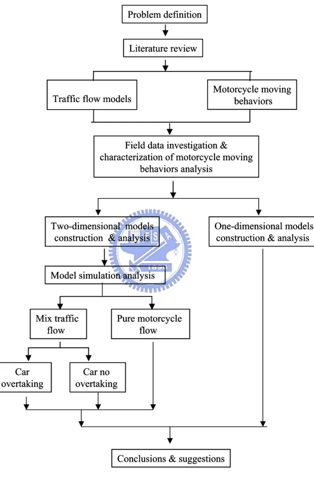
(15) (3) Field investigation and analysis This study conducts field observations and analyses on motorcycles’ moving characteristics. In order to capture the interactive behaviors between motorcycles and surrounding vehicles (including cars and motorcycles) and trajectories of vehicles, mixed traffic flow is photographed by a video camera fixed on a high building. The video camera is placed not to be obstructed by billboards or trees. From the field data, this study measures the detailed positions, speeds, accelerations and gaps between motorcycles and surrounding vehicles, etc. Statistical methodology such as correlation analysis will be used to analyze the characteristics of the field data. (4) Modeling the one-dimensional moving Significant factors affecting the motorcycle-following behaviors, based on the observation, will be selected to construct the fuzzy-based one-dimensional moving models that can properly reflect motorcycle’s acceleration rates associated with these factors. The comparison between GM car-following model and our proposed fuzzy-based model is presented. (5) Modeling the two-dimensional moving The CA model is capable of imitating the positions of vehicles over time and space, this study will further develop two-dimensional CA models in such a way that the speed of each vehicle (car or motorcycle) changes in discrete time steps as a consequence of its interactions with other vehicles. Each vehicle follows certain pre-assigned rules that govern the positions of the vehicle over time and space, depending on various circumstances. Moreover, we employ the CA models to simulate mixed traffic flow with various percentages of passenger cars under various lane width scenarios. (6) Conclusions and suggestions The major findings from field observation and from both one- and two-dimensional moving models are summarized and the directions for future studies will be suggested.. 4.

(16) Problem definition Literature review. Motorcycle moving behaviors. Traffic flow models. Field data investigation & characterization of motorcycle moving behaviors analysis. Two-dimensional models construction & analysis. One-dimensional models construction & analysis. Model simulation analysis. Mix traffic flow. Car overtaking. Pure motorcycle flow. Car no overtaking. Conclusions & suggestions. Figure 1-1 Research procedures 5.

(17) 1.4 Chapters Organization This study is organized as follows. Chapter one briefly points out the importance of motorcycle moving behavior study, particular in the mixed traffic contexts. Chapter two overviews the previous related works on traffic flow models and motorcycle flow studies. Chapter three elaborates our proposed research methodologies, including fuzzy-based and CA models. Chapter four carries out a field observation with detail analysis on the characteristics of motorcycle moving in mixed traffic. Chapter five constructs models for the one-dimensional motorcycle moving behaviors. A comparison of GM model and our proposed fuzzy-based model is performed. Chapter six further constructs models for the two-dimensional motorcycle moving behaviors. Both deterministic and stochastic CA models are attempted and validated. Chapter seven summarizes the conclusions and addresses issues for further studies.. 6.

(18) CHAPTER 2 AN OVERVIEW OF RELATED WORKS In this chapter, we overview the traffic flows modeling, including conventional flow models and recent cellular automaton (CA) models. Then we briefly investigate the works relating to motorcycles and then provide with some comments. 2.1 Traffic Flow Models (1) Conventional traffic flow models Conventional traffic flow models can be roughly separated into three branches: macroscopic models, mesoscopic models and microscopic models. The macroscopic models include traffic flow models and fluid-dynamical models. Traffic flow models, single-regime or multiple-regime, are mostly devoted to the relations between speed, density and volume (May, 1990). Fluid-dynamical models, on the other hand, analogize vehicular flow to fluids and assume the aggregate behavior of drivers depending on the traffic conditions. Lighthill and Whitham (1955) and Richard (1956) developed the most well-known one-order fluid-dynamical models; high-order fluid-dynamical models were derived by other researchers, for example, Payne (1971), Liu, et al. (1998) and Zhang (1998). Mesoscopic models aim to describe the behavior of small groups of vehicles. Examples of these models are the so-called cluster models and the gas-kinetic models. Prigogine & Herman (1971) summarized possible alternate forms of the relaxation term in their kinetic equation of vehicular traffic. They derived the Lighthill-Whitham situation as limiting case of the kinetic theory. Hoogendoorn and Bovy (1999) proposed a traffic flow model describing multilane heterogeneous (i.e. unconstrained and constrained) traffic flow. It was observed that these dynamic changes are causes by both continuum and noncontinuum processes. The former processes are caused by the flow of constrained and unconstrained vehicles in the phase space and the consequent changes. However, the latter processes are caused by vehicles decelerating after interacting, immediate lane changing, spontaneous lane changing and postponed lane changing. Alternate kinetic models that have been proposed to eliminate perceived. 7.

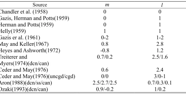
(19) deficiencies of the Prigogine & Herman model have subsequently been accepted by a number of researchers, most notably by Paveri-Fontana (1975) and Phillips (1979), and more recently by Nelson (1995), and Nelson and Sopasakis (1998). The microscopic models describe the behavior of an individual vehicle with respect to other vehicles in the traffic stream. Car-following theory is the pertinent model that describes microscopic behavior of any two vehicles traveling in a longitudinal lane such that the following vehicle adjusts its speed to maintain desirable or safe distance headway with the lead vehicle. Car-following models can be expressed as some mathematical equations that represent the interrelationship of motion between lead and following vehicles (May, 1990). The types of car-following models are in general divided into four categories: A. Stimulus-response This model is the most well-known model and dates from the late fifties and early sixties. It formulation is a n ( t ) = cv nm ( t ). ∆ v (t − T ). (2.1). ∆ x l (t − T ). where a n and v are the acceleration and speed of vehicle n implemented at time t by a driver; ∆x and ∆v are the relative spacing and speed between the n th and n − 1 th vehicle; T is the driver reaction time; and c, m, l are the constants to be determined. Several similar investigations occurred during the following 15 years, in the attempt to define the ‘best’ combination of m and l . A summary of the varying parameter combinations to emerge from research on the equation is given in Table 2.1. (Brackstone and McDonald, 1999). 8.

(20) Table 2.1 Summary of optimal parameter combinations for stimulus-response equation m Source l Chandler et al. (1958) 0 0 Gazis, Herman and Potts(1959) 0 1 Herman and Potts(1959) 0 1 Helly(1959) 1 1 Gazis er al. (1961) 0-2 1-2 May and Keller(1967) 0.8 2.8 Heyes and Ashworth(1972) -0.8 1.2 Treiterer and 0.7/0.2 2.5/1.6 Myers(1974)(dcn/can) Ceder and May(1976) 0.6 2.4 Ceder and May(1976)(uncgd/cgd) 0/0 3/0-1 Aron(1988)(dcn/ss/can) 2.5/2.7/2.5 0.7/0.3/0.1 Ozaki(1993)(dcn/can) 0.9/-0.2 1/0.2 Notes: dcn/can: deceleration/ acceleration; bek/no brk: deceleration with and without the use of brakes; uncgd/cgd: uncongested/congested; ss: steady state. Source: Brackstone and McDonald (1999). B. Safety distance The original formulation of this approach dates to Kometani and Sasaki (1959). The base relationship did not describe a stimulus-response type function, but sought to specify a safe following distance, within which a collision would be unavoidable, if the driver of the vehicle in front were to act ‘unpredictably’. The original formulation is as follows: ∆x(t − T ) = αv n2−1 (t − T ) + β 1v n2 (t ) + βv n (t ) + b0. (2.2). The next major model was made by Gipps (1981). He considered several mitigating factors that earlier formulation neglected. These were that drivers will allow an additional ‘safety’ reaction time to T/2, and that the kinetic terms in the above formula are related to braking rates of − 1 / 2bn , bn , the maximum braking rate that the driver of the n th vehicle wishes to use, and − 1 / 2b * , b * , the maximum braking rate of the n − 1 th vehicle that the n th driver believes is likely to be used. C. Action point The first discussion of the underlying factors that would eventually lead 9.

(21) to the construction of these models was given by Michaels and Cozan (1963), who raised the concept that drivers would initially be able to tell they were approaching a vehicle in-front, primarily due to changes in the apparent size of the vehicle, by perceiving relative velocity through changes on the visual angle subtended by the vehicle ahead θ . The threshold for this perception is well-known in perception literature and given as, d / dt (~ ∆v / ∆x 2 ) ~ 6 × 10 − 4 . Once this. threshold is. exceeded , drivers will chose to decelerate until they can no longer perceive any relative velocity, and provided the threshold is not then re-exceeded, will base all their actions on whether they can then perceive any changes in spacing. Evans and Rothery (1973) developed models through a series of perception-based experiments conducted in early seventies and aimed at quantifying the thresholds. A review of many investigations conducted in these areas at that time can be found in Evans and Rothery (1977), where it is shown that the wide body of research conducted on this topic during the seventies are all consistent from a statistical point of view. Hsu and Chiang (2002) developed MUMO-MISS (Multi-Mode Microscopic Simulation System) to simulate multi modes traffic based on action points. It is difficult to come to a firm conclusion as to the validity of these models, as although the entire system would seem to simulate behavior acceptably, calibration of the individual elements and thresholds has been less successful. D. Fuzzy logic based In the car following situation, one follows a set of driving rules built over time through experience. These models are a response to concern that drivers do not exercise the dichotomous decision criteria assumed in the traditional deterministic car following models. They have the following characteristics: Driver’s decision criteria are dealt with by fuzzy inference logic, which allows several decision rules to fire at the same time for a given set of input. As a result, the final output incorporates the ambiguity of the decision process. 10.

(22) The inference rules a collection of natural language based straightforward driving rules. The number of rules can be adjusted, and each rule can be independently modified to suit the decision criteria. The output is a fuzzy number that represents a range of possible acceleration (or deceleration) rates of the following vehicle. The result is realistic and consistent with the general expectation from a car following model: for the same final speed, the distance between leading vehicle and following vehicle eventually converges to the same value regardless of the initial condition. The “drift,” oscillation of the distance between leading vehicle and following vehicle, can also be captured. Chakroborty and Kikuchi (1999) proposed a model that used fuzzy inference system to predict the reaction of the driver of the following vehicle. A range of possible reaction is predicted and expressed by fuzzy membership function. The model is applied to analyze the traffic stability and speed-density relationship. Lan, et al. (1994) proposed the model based on the relative speed, distance and speed of following vehicle and found that the proposed model can improve the Chakroborty and Kikuchi’s mdoel. Lan and Yeh (2001) attempted design an adaptive neuro-fuzzy inference system which is characterized with learning ability to modify the membership functions of distance headways and relative speeds. It is found that a near stable distance headway will be obtained for each cluster of drivers. More aggressive drivers tend to have shorter distance headways and require less time to reach stable conditions. Chiou and Lan (2001) developed a genetic fuzzy logic controller model with iterative evolution of genetic algorithms to improve the parameter determinations of membership functions and found that the model can predict car following behaviors precisely. Among these four categories, perhaps the most pertinent model is the stimulus-response type that was developed in the 1950s and 1960s by the General Motors (GM) research group. Five generations of GM car-following models are recognized, and they are still applied in various aspects, including traffic stability and safety studies, level of service and capacity analyses, driver reaction times, etc.. 11.

(23) The lane-changing model for an individual vehicle is another microscopic model. According to motives of driver, lane-changing behaviors could be divided into optional lane changing and forced lane changing behaviors. The former behaviors expect to achieve a desired speed, and the latter behaviors expect to achieve the desired lane. Most of related researches focused on constructing a reasonable lane changing decision-making model. Gipps (1986) proposed a framework for the structure of lane changing decisions in urban driving situations including the influence of traffic signals, obstructions and different vehicle types such as heavy vehicles. The model concentrated on the decision-making process and described drivers’ lane changing maneuvers which assume that a lane changing maneuver takes place without interference with vehicles in the destination lane. The decision whether or not to change lane was based on the following factors in Gipps’ model: Whether it is physically possible and safe to change lanes without an unacceptable risk of collision; The location of permanent obstructions; The presence of special purpose lanes such as transit lanes; The driver’s intended turning movement; The presence of heavy vehicles; and The possibility of gaining a speed advantage.. However, lane changing could never occur in a congested situation according to the rules. While Gipps’ model provided a convenient starting point for the implementation of the lane changing algorithms in Simulation of Intelligent Transport Systems (SITRAS). As compared with the commonly rule-based methods, a different approach was taken by Hunt and Lyons (1994). They developed a driver decision-making model for lane changing using neural networks. Their model works by assessing simple visual pattern-based input describing the driving environment around the vehicle about to change lane; it did not consider possible cooperation between drivers during lane changing. Yang and Koutsopoulos (1996) proposed a simulation model which explicitly addressed cooperative lane changing with using a courtesy function to make space for a vehicle moving into the lane. The concept appeared to be similar to that implemented in 12.

(24) SITRAS. Van Winsum et al.(1999) presented evidence that drivers who are less able to perceive difference in the Time-to-Line-Crossing (TLC) to the lead vehicle compensate for this by following other vehicles at a larger distance. The results suggested that visual feedback is used during the lane change maneuver in order to adjust steering control actions to the outcome of a previous action in such a way that safety margins are controlled. Moreover, the results suggested that temporal information about the relation between the vehicle and the lane boundaries is used by the driver to control the motor response. Similar relations between perception and action have been demonstrated in other studies for the case of curve negotiation and for braking in response to a decelerating lead vehicle in car-following. Hashimoto et al. (2001) investigated the mechanism of drivers’ hazard judgment for lane change decision. Subjects were tested to determine a critical inter-vehicle gap by which the subject judges between safe and unsafe lane changes. Then, a regression equation to correlate the critical gap and relevant vehicle state variables was obtained. It is shown that the equation’s structure paralleled the subjects’ hazard perception mechanism and its parameters corresponded with their judgment criteria. Hidas (2002) introduced Simulation of Intelligent Transport Systems (SITRAS), a massive multi-agent simulation system in which driver-vehicle objects are modeled as autonomous agents, and presented the details of the lane changing and merging algorithms developed for SITRAS model. These models incorporated procedures for ‘forced’ and ‘co-operative’ lane changing which are essential for lane changing under congested traffic conditions. The results indicated that only the forced and cooperative lane changing models producing realistic flow-speed relationship during congested conditions. Tsao and Su (1994) investigated the characteristics of forced lane changes by off-ramp vehicles departing from an urban expressway and used the concept of lag to establish the criteria for an off-ramp vehicle to make a decision to change lane. A step-wise regression technique was used to derive the relationships between traffic flow variables after and before the forced lane change. Results showed that the accuracy of the proposed model was about 89%. Hwu (1993) studied the behavior about lane change of the vehicle on the freeway, including choice and track model of lane changing vehicles, and reaction of other drivers. Firstly, he established binary choice model according to the gap between lane changing vehicle and its leading vehicle, the gap between the leading vehicle of near lane and following vehicle of near lane, the distance between lane changing 13.

(25) vehicle and its following vehicle, the relative velocity between the lane changing vehicle and the following vehicle of near lane. Secondly, he established the track model with angle model and acceleration model. Chen (1997) constructed a traffic simulation model by artificial neural network learning driver’s car-following and lane-changing behaviors based on the traffic data which was obtained in virtual reality experiments on a prototype driving simulator. Summary major factors of related researches include speeds of vehicle, relative speeds, relative positions, acceptable gaps and obstacles. (2) Cellular automata (CA) models Recently, various types of micro-simulation models have been proposed to simulate the microscopic behaviors of a particle (vehicle) moving according to some pre-assigned cellular automata (CA) parallel update rules. A CA model has a number of identical cells, each interacting with a few nearby neighbors by simple rules. The rules can be deterministic or probabilistic (random). Each cell is in one of a small number of discrete states. Time advances in distinct steps and the cell states are updated either s synchronously (all at once) or asynchronously (either randomly or sequentially). Krug and Spohn (1988) derived a simultaneous moving model for all particles with maximum speed defaulted as 1 m/sec. This model is also called CA-184 rule because it corresponds to Rule 184 in Wolfram’s classification (Wolfram, 1986). If the particle-hopping model controls only one particle’s moving in random for each time step, it is called an asymmetric stochastic exclusion process (ASEP). The NcSch model, proposed by Nagel and Schreckenberg (1992), is perhaps the pioneering CA traffic model, which combines the behavior ASEP and CA-184.Nagel and Herrmann (1993) studied several one-dimensional deterministic traffic models. For integer positions and velocities, it found that the typical high and low density phases separated by a simple transition. Nagatani (1993) investigated the effect of two-level crossings on the traffic jam in CA model of traffic flow. It found that the dynamical jamming transition does not occur when the fraction c of the two-level crossings becomes larger than the percolation threshold; however, the dynamical jamming transition occurs at higher density of cars with increasing fraction c of the two-level crossings below the percolation threshold. Nagel (1994) investigated traffic jams which emerge in a natural way from a rule-based, cellular-automata-like 14.

(26) traffic model when operating the model near the maximum traffic throughput. The model includes strong driving by noise taking into account the strong fluctuations of traffic. The lifetime distribution of these jams showed a short scaling regime, which gets considerably longer if one reduces the fluctuations when driving at maximum speed but leaves the fluctuations for slowing down or accelerating unchanged. The outflow from traffic jam self-organized into this state of maximum throughput. A series of studies employ the stochastic traffic cellular automaton (STCA) by treating each particle with randomized integer speed between 0 and vmax (Nagel, 1996; 1998). The findings of these papers have some fairly far-reaching implication including robust numeric, universality, toward minimal models, traffic dynamics, for traffic simulation models. Nagel, et al. (1998) summarized different approaches to lane changing and their results for freeway traffic. This paper separated the lane changing principles into incentive part and traffic control strategies part. The former asks if there is enough space available in the target lane, and the latter is the observation with a default lane and a passing lane. Furthermore, this paper proposed a general scheme by applying it to several different lane changing rules, which, in spite of their differences, generate similar and realistic results. Besides, the findings of this paper also showed both velocity- and gap-based implementations of give satisfying results. Rickert, et al. (1996) examined a simple two-lane cellular automaton based upon the single-lane CA introduced by Nagel and Schreckenberg. They pointed out important parameters defining the shape of the fundamental diagram; moreover, they investigated the importance of stochastic elements with respect to real life traffic. Chowdhury, et al. (1997) developed a particle-hopping model of two-lane traffic with two different types of vehicles generalizing the NcSch stochastic CA model. Hermann and Kerner (1998) applied CA technique and self-organization process to explore the formation of traffic congestion. Wolf (1999) employed the modified NcSch model to discuss the meta-stable states at the jamming transition in detail. And this paper showed the interaction between cars is Galiliei-invariant. Schadschneider (2000) pointed out that CA models have big advantage of being ideally suited for large-scale computer simulations. It offers new perspectives for the planning and design of transportation networks. Wang, et al., (2000) introduced the NcSch model and the Fukui-Ishibashi (FI) model to discuss the asymptotic self-organization phenomena of one 15.

(27) dimension traffic flow. Pottmeier, et al., (2002) studied the impact of localized defects in a CA model for traffic flow which exhibits meta-stable states and phase separation. More recently, Bham and Benekohal (2004) develop a traffic simulation model based on CA and car-following concepts, which has been satisfactorily validated at the macroscopic and microscopic levels using two sets of field data. Validation at the macroscopic level has been performed for average speed, density and volume. Validation at the microscopic level has been conducted for trajectory and speed of individual vehicles. Daganzo (1994) develops cell transmission model in which the highway is partitioned into small cells and vehicles move in and out of these cells over time. However, it is not necessary to know where the vehicles are located within the cell, which is essentially different from the rationales for cellular automata. 2.2 Motorcycles’ Related Works (1) Driving behavior Ju (1999) undertook to explore the reaction of motorcyclists in facing traffic conflicts based on an established conceptual framework and experimental surveys. That study introduced the conceptual framework, which could apply to both motorcycles and cars, involving both psychology (reactions and decisions) and visible behaviors that could be observed and measured. We will indirectly explore the rules of decision making of motorcyclists based on these measures. (2) Characteristics of motorcycles’ moving Many researchers have described the specific characteristics of motorcycles’ moving behavior in Taiwan. These researches could be divided into three types: flow characteristics of motorcycle lanes, basic characteristics of motorcycles in mixed traffic flow, and traffic engineering and traffic management strategies. A. Flow Characteristics of Motorcycle Lanes Lin (1979) analyzed the characteristics of motorcycle flow and found the saturation flow rate of motorcycles was 0.5 sec/veh based on field data collected on Tientsin Street in Taipei City. Tang (1998) discussed 16.

(28) the characteristics of motorcycle lanes with different widths. He proposed that, according to the expected motorcycle speed, the width of the motorcycle lane should be designed differently. Tang (2001) investigated the discharging pattern of pure motorcycle flow in intersections. The results show that the discharging of motorcycle flow became steady from the green light to 12 seconds, and the saturation discharge rate for motorcycle lane with 3 m-widths was 4.22 veh/2sec/3m. B. Characteristics of Motorcycle in Mixed Traffic Flow Chiou (1995) defined the M.D.E (motorcycle delay equivalence), which takes the cars occupying the motorcycle stop location and extrapolates a value using the floating car method in order to apply it to irregular waiting configurations. By using the cumulative curve method to measure motorcycle delays under six conditions with different arrivals, departures and waiting configurations, Chen (1993) presented the concept of the behavioral threshold model. Moreover, he modeled the logic of interactive behavior for motorcycles based on field data, but did not conduct model validation. Hsu et al. (2001) defined the noise of motorcycles’ moving trajectories according to field observations and the characteristics of accidents. They also established a ‘Dummy Lane variation of motorcycles (△DL)’ as an index for measuring motorcycle traffic flow. Hsu et al. (1995) proposed a concept of lining the space of motorcycle movement, and elaborated the attributes of flow in motorcycle lanes. Hsu and Cheng (1999) compared the running speed, approaching speed and accepted gaps of motorcycles with those of cars. It was found that speeds of motorcycles are higher than cars, and accepted gaps between motorcycles are shorter than cars. Powell (2000) amended a first order macroscopic model tested against video data of motorcycles collected at intersections in Indonesia, Malaysia and Thailand to describe motorcycle behavior at intersections. The model predicted the number of QFLIER1 per cycle with a high degree of accuracy. Chiou and Sheu (1992) constructed a simulation model which used a 1. QFLIER – Motorcycle which sets off from the front of the queue before the end of the first 6 seconds of effective green time. 17.

(29) two dimensional coordinate to simulate vehicle movement. Based on the dynamic lengths and widths of the vehicle, movement is simulated by considering directional movement, road-width, the presence of front vehicles, and signal control. The simulation results showed that simulated trajectories of vehicles mesh reasonably well with observed characteristics. Hwang and Ho (1994) introduced fuzzy logic theory to model complicated driving behaviors on the road. They also proposed the concept of the “crisscross squares fuzzy moving forward method” to represent dimensions and movements of different vehicles. Lin (2002) tried to develop a motorcycle traffic flow model based on a field observation by using neural network method. After detailed data analyzing, the motorcycle progress path has been divided into two dimensions, i.e. longitudinal moving and transversal moving model. It found that longitudinal progress model performs better than the traversal progress model. C. Traffic Engineering and Traffic Management Strategies The Institute of Transportation (2001) conducted an investigation of their own field data, and proposed a procedure for the valuing of safety and efficiency. Because the results of the study have proven effective for the municipalities in executing motorcycle lane policy, they should then serve as good references in determining the locations of motorcycle lane. Hsu et al., (1998, 2001) found that setting up motorcycle stopping areas at intersections can increase the efficiency of motorcycle discharge, based on the comparisons of start delay, discharge rate and saturation flow rate of motorcycles.. 2.3 Some Comments The above-mentioned conventional macroscopic, mesoscopic and microscopic traffic flow models were developed mainly for depicting the moving behaviors of cars. Little was devoted to motorcycles moving in mixed traffic flow. As stated in chapter one, motorcycles do not necessarily move along a specified lane. Hence, conventional flow models may not accurately capture such motorcycles’ moving behaviors in mixed traffic. Previous CA traffic models define the cell unit as 7.5×7.5 meters square grid and assume that each particle 18.

(30) has identical size occupying one cell unit; namely, the space required for each vehicle is 7.5 meters both in length and in width. Because the definition of cell unit is too coarse, vehicles are modeled as particles with abrupt speed jumps or drops, which are too far apart from the real-world situations. Although these simple and well-understood particle models can generate the most phenomena of an individual particle, previous CA models were also developed mainly for depicting the moving behaviors of cars. None have been devoted to motorcycles moving in mixed traffic flow. Many researches in Taiwan have described the related characteristics of motorcycles’ for specific purposes. These researches could be divided into three areas: flow characteristics in motorcycle lanes, characteristics of motorcycles in mixed traffic, and traffic engineering and traffic management strategies. In the first area, they conclude that pure motorcycle flow can be interpreted by macroscopic concepts (or models). Other related works focus on specified traffic engineering management purposes and may not elaborate the moving behaviors for motorcycles. Little has dealt with both pure and mixed traffic flow with regards to motorcycles.. 19.

(31) 20.

(32) CHAPTER 3 PROPOSED METHODOLOGIES This chapter proposes methods for modeling the one-dimensional motorcycles’ longitudinal moving behaviors and two-dimensional motorcycles’ longitudinal moving and latitudinal shift behaviors. Section 3.1 presents the one-dimensional moving methodologies, including GM-based and fuzzy-based models. Section 3.2 introduces the CA models for describing the longitudinal moving and lateral displacement behaviors for motorcycles. 3.1 Methods for Modeling the One-dimensional Moving Behaviors Car-following is a major microscopic behavior for vehicles’ longitudinal motions, in which any two vehicles traveling in a longitudinal lane such that the following vehicle adjusts its velocity to maintain desirable or minimum safety distance headway with the lead vehicle. Previous GM based and fuzzy-based following models have mainly dealt with the motion of such vehicles as passenger cars, buses and trucks. These types of vehicles tend to travel within a longitudinal lane. Very little has been devoted to the motion of motorcycles. Motorcyclists tend to sneak among different longitudinal lanes with frequent lateral displacement; therefore, car-following models may not be appropriate to depict motorcycle behaviors. Nevertheless, there still exist some motorcycles in “following” manner that the following motorcycles interact with the lead vehicles at safety distance headway. Thus, it is worthy to construct appropriate models to gain insights of motorcycle-following behaviors. Hence, this study presents the methodologies of GM models and fuzzy-based following models for motorcycles in this section. 3.1.1 GM models Five generations of GM car-following models are well recognized and they take the common form as: response = sensitivity × stimulus. The response term is represented by the acceleration or deceleration of the following vehicle. The stimulus term is represented by relative velocity of the lead and following vehicles. The only difference in these five-generation models is the sensitivity term, which ranges from a constant (the first generation) to a combination of speed and distance headway of the following vehicle, both to some generalized exponents (the fifth generation).. 21.

(33) The fifth generation of GM car-following model takes the form as follows:. an +1 (t + ∆t ) =. α [Vn +1 (t + ∆t )]m ∆S l. [Vn (t ) − Vn +1 (t )]. (3.1). where. an +1 (t + ∆t ) = acceleration rate of the following vehicle at time t + ∆t. [Vn (t ) − Vn +1 (t )] = relative velocity of the lead vehicle and the following vehicle at time t ∆S = space headway between the lead vehicle and the following vehicle Vn +1 (t + ∆t ) = velocity of the following vehicle at time t + ∆t. α , m, l = parameters to be estimated. This model has the following characteristics: (1) The interaction between stimulus and reaction has a one-to-one correspondence. The notion that a driver’s reaction pattern is imprecise is not fully represented. Representation of a human behavioral pattern may be better explained by an approximate reasoning process than a deterministic model. (2) The following vehicle reacts even to minute changes in relative velocities between leading vehicle and following vehicle in a deterministic manner. (3) Sensitivities of the following vehicle to the positive and negative relative velocities are the same. The GM researchers have devoted to comprehensive field experiments and the discovery of the mathematical equations of motion has bridged between microscopic and macroscopic traffic flow theories. Through the mathematical equations, the trajectory of the following vehicle over space and time as a function of the trajectory of the lead vehicle can be tracked. Even today, such GM car-following theories are still widely applied in various aspects, including traffic stability and safety study, level of service and capacity analysis, driver’s reaction times, etc.. 22.

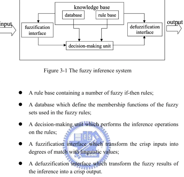
(34) 3.1.2 Proposed fuzzy- based models System modeling based on conventional mathematical tools is not well suited for dealing with ill-defined and uncertain systems. By contrast, a fuzzy inference system employing fuzzy if-then rules can model the qualitative aspects of human knowledge and reasoning processes without employing precise quantitative analyses. The fuzzy modeling, first explored systematically by Taksgi and Sugeno (1985), has found numerous practical applications in control, prediction and inference. However, there are some basic aspects of these approaches which are in need of better understanding. More specifically: No standard methods exist for transforming human knowledge or experience into the rule base and database of a fuzzy inference system. There is a need for effective methods for tuning the membership functions so as to minimize the output error measure or maximize performance index. In this perspective, the adaptive network based fuzzy inference system can serve as basis for constructing a set of fuzzy if-then rules with appropriate membership functions to generate the stipulated input-output pairs. The fuzzy inference systems and structure are introduced as follows. (1) Fuzzy inference systems Fuzzy inference systems are also knows as fuzzy-rule-based systems, fuzzy models, fuzzy associative memories, or fuzzy controllers when used as controllers. Basically a fuzzy inference system is composed of five functional blocks (see Figure 3-1). 23.

(35) knowledge base database. input. rule base defuzzification interface. fuzzification interface. output. decision-making unit. Figure 3-1 The fuzzy inference system. A rule base containing a number of fuzzy if-then rules; A database which define the membership functions of the fuzzy sets used in the fuzzy rules; A decision-making unit which performs the inference operations on the rules; A fuzzification interface which transform the crisp inputs into degrees of match with linguistic values; A defuzzification interface which transform the fuzzy results of the inference into a crisp output. Usually, the rule base and the database are jointly referred to as the knowledge base. The steps of fuzzy reasoning (inference operations upon fuzzy if-then rules) performed by fuzzy inference systems are: Compare the input variables with the membership function on the premise part to obtain the membership values (or compatibility measures) of each linguistic label. (This step is often called fuzzification). Combines (through a specific T-norm operator, usually multiplication or min.) the membership values on the premise part to get firing strength (weight) of each rule. Generate the qualified consequent (either fuzzy or crisp) of each rule depending on the firing strength.. 24.

(36) Aggregate the qualified consequents to produce a crisp output. (This step is called defuzzification.) Sugeno’s fuzzy if-then rules (1985) are used in this study. The output of each rule is a linear combination of input variables plus a constant term, and the final output is the weighted average of each rule’s output. A typical fuzzy rule in Sugeno fuzzy model has the form:. if x is A and y is B then. z = f ( x, y ) ,. where A and B are fuzzy sets in the antecedent, while z = f ( x, y ) is a crisp function in the consequent. Usually f ( x, y ) is a polynomial in the input variables x and y , but it can be any function as long as it can appropriately describe the output of the model within the fuzzy region specified by the antecedent of the rule. When the f ( x, y ) is a first-order polynomial, the resulting fuzzy inference system is called a first-order Sugeno fuzzy model. Figure 3-2 shows the fuzzy reasoning procedure for a first-order Sugeno fuzzy model. Since each the rule has a crisp output, the overall output is obtained via weighted average.. µ. A1. µ. B1. X. µ. A2. w1. z1 = p1x + q1 y + r1. w2. z2 = p2 x + q2 y + r2. Y. µ. B2. X. Y w z + w2 z2 z= 11 w1 + w2 = w1z1 + w2 z2. Figure 3-2 Reasoning of Sugeno fuzzy model. 25.

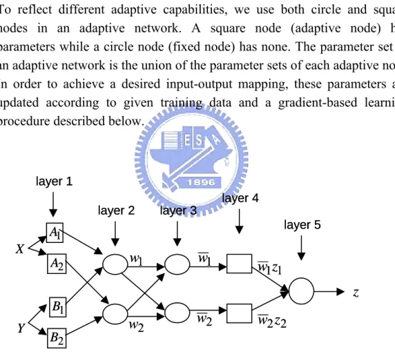
(37) (2) Architectures and learning algorithms An adaptive network is a multiplayer feed-forward network in which each node performs a particular function on incoming signals as well as a set of parameters pertaining to this node. (see Figure 3-3) The formulas for the node functions may vary from node to node, and the choice of each node function depends on the overall input-output function which the adaptive network is required to carry out. Note that the links in an adaptive network only indicate the flow direction of signals between nodes; no weights are associated with the links. To reflect different adaptive capabilities, we use both circle and square nodes in an adaptive network. A square node (adaptive node) has parameters while a circle node (fixed node) has none. The parameter set of an adaptive network is the union of the parameter sets of each adaptive node. In order to achieve a desired input-output mapping, these parameters are updated according to given training data and a gradient-based learning procedure described below.. layer 1 layer 4 layer 2. layer 3 layer 5. A1 X. w1. A2. w1. w1z1 z. B1 Y. w2. B2. w2. w2 z2. Figure 3-3 Adaptive network for fuzzy model. 3.1.3 A comparison GM car-following theories assume that all drivers are identical; namely, each driver takes the same actions (accelerates, decelerates, or remains constant velocity) once he or she perceives the same amount of stimulus. In the real. 26.

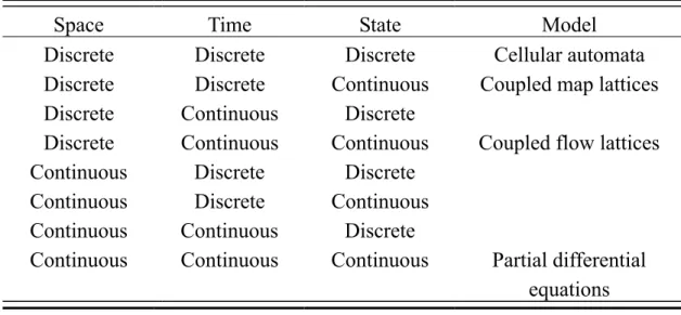
(38) world, unfortunately, this assumption may not be valid because one can easily find that some drivers (risk-taking) may follow the lead vehicle rather closely while the others (risk-aversion) are far apart from the lead vehicle. In other words, each driver may respond differently even perceiving the same amount of stimulus. To deal with the risk diversity of drivers’ reactions, recent researches have introduced fuzzy inference with neural network to the car-following models. Such fuzzy-based models have been proven more realistic than GM based models in capturing the risk heterogeneity over the whole driver population. 3.2 Methods for Modeling the Two-dimensional Moving Behaviors The modified CA models are introduced to describe the interaction between vehicles, including longitudinal moving and lateral displacement behaviors. The basic definition for CA models will be presented firstly; the proposed CA model follows. 3.2.1 Basic definition for CA models The CA model, in which everything is discrete, is the simplest model of spatiotemporal models. The various spatiotemporal models can be categorized according to whether space, time, and the state of the variables are quantified, as summarized in Table 2.2. (Sprott, 2003) Table 2.2 Summary of spatiotemproal models Space Discrete Discrete Discrete Discrete Continuous Continuous Continuous Continuous. Time Discrete Discrete Continuous Continuous Discrete Discrete Continuous Continuous. State Discrete Continuous Discrete Continuous Discrete Continuous Discrete Continuous. Source: Sprott, J. C. (2003).. 27. Model Cellular automata Coupled map lattices Coupled flow lattices. Partial differential equations.

(39) The common forms for one-dimension CA system with n cells and r interactive range are indicated as:. ai − r , ai −r +1 , … , ai ,…, ai +r −1 , ai + r the dynamic function is discrete on time as follows:. ai(t ) =[ ait−−1r , ait−−1r +1 , … , ait −1 , …, ait+−1r −1 , ait+−1r ] (3.2) where,. ai = the ith cellular value, i = 1 ~ n. t = t time step, r = interactive range.. a i = {0,1} , F：{0, 1}2r+1→{0, 1}. Based on a definite rule (i.e. Eq. (3.2)), the value of ai will be determined. At each time step t, every cell’s state depends on the states of its neighbors (cells in interactive range) at time step t − 1. The system can be very complex after a lot of time steps with propagation law. For example, in the NaSch model (1992), which is a one-dimension CA system, each cell can be empty or occupied by one car (i.e. a i = 0 indicates the cell is empty, a i = 1 indicates the cell is occupied). 3.2.2 Proposed CA models Considering the different particles in mixed traffic flow and both longitudinal moving and latitudinal shift behaviors, this study will employ a modified two-dimension CA model to model motorcycle’s moving behaviors in mixed traffic flow. The following key rules will be defined according to the field observation. time step; size of cell; 28.

(40) particles’ dimension (including motorcycles and cars, see Figure 3-4) maximum speed; y. x :motorcycle. :car. Figure 3-4 Two-dimension CA model for mixed traffic flow. position update for every time step according to following rules A. speeds update for every time step find the gap dX tf between the i. th. particle and front. particle at t time step，if a. dX tf is enough to accelerate or keep maximum speed then. new speeds are as follows: (i.e. dX tf > v × 1). [. Vi t +1 = Min Vi t + (1,0), (v max ,0). ]. where,. Vi t = (v,0) = vx + 0 y is speed of the i th particle at t time step in ( x, y ) two-dimension space;. Vi t +1 is speed of the i th particle at t + 1 time step;. v max is the maximum speed. b. dX tf is not enough to accelerate or keep maximum speed,. 29.

(41) and the spaces on lateral adjacent line are enough to move to, that is, the particle (vehicle) moves to the targeted lane and will not make any collision, new speeds are as follows:. Vi t +1 = Vi t + PC where, PC is the vector for changing lateral position,. while particle move left PC = (0,1) , and move right PC = (0,−1) . c. dX tf is not enough to accelerate or keep original speed, and the spaces on lateral adjacent line are to, then new speeds are as follows:. not enough to move. Vi t +1 = (dX tf ,0) B. movement, each vehicle is moved forward according to its new velocity.. Pi t +1 = Pi t + Vi t +1 where, Pi t is the position of the i th particle at t time. Pi. t +1. step; is the position of the i th particle at t + 1 time step.. 30.

(42)