模糊邏輯控制於語者調適及音訊事件偵測之參數調適

國

立

交

通

大

學

資訊科學與工程研究所

博 士 論 文

模糊邏輯控制於語者調適及

音訊事件偵測之參數調適

On the Use of Fuzzy Logic Control in Adaptive Parameter

Tuning for Speaker Adaptation and Audio Event Detection

研 究 生：丁英智

指導教授：林正中 教授

模糊邏輯控制於語者調適及音訊事件偵測之參數調適

On the Use of Fuzzy Logic Control in Adaptive Parameter

Tuning for Speaker Adaptation and Audio Event Detection

研 究 生：丁英智 Student：Ing-Jr Ding

指導教授：林正中 Advisor：Cheng-Chung Lin

國 立 交 通 大 學

資 訊 科 學 與 工 程 研 究 所

博 士 論 文

Submitted to Institute of Computer Science and Engineering College of Computer Science

National Chiao Tung University in partial Fulfillment of the Requirements

for the Degree of Doctor of Philosophy

in

Computer Science and Engineering

December 2008

Hsinchu, Taiwan, Republic of China

模糊邏輯控制於語者調適及音訊事件偵測之參數調適

學生：丁英智 指導教授：林正中 博士

國立交通大學 資訊科學與工程研究所

摘

要

本篇論文在語者調適(speaker adaptation, SA)領域及音訊事件偵測(audio event

detection)領域中導入了模糊邏輯控制(fuzzy logic control, FLC)機制以強化調適品 質，從而改善自動語音辨識(automatic speech recognition, ASR)系統及音訊事件辨 認(audio event recognition)系統的辨識性能。個人提出了數個結合模糊邏輯控制器 的方法以有效地掌控辨識系統中的不定參數，進而使系統在處於極為不利的辨識 情況時仍能保持令人滿意之辨識結果。對於語者調適領域，個人針對兩個廣為流 傳的調適技術範疇：貝氏調適(Bayesian-based)及轉換調適(transformation-based) 置入 FLC 調控機制。最大後機率(maximum a posteriori, MAP)估測調適是一種貝 氏調適的典型方法。根據 MAP 方法，個人提出了結合一適當的模糊控制器的

FCMAP 方法。所發展之 FCMAP 可以藉由所設計的模糊控制器依據調適語料量 之多寡有效地糾正隱藏式馬可夫模型(hidden Markov model, HMM)參數。然而，

MAP 僅針對調適語料所涉及的 HMM 參數進行調適的改善，對於絕大部份沒有 調適語料的 HMM 參數並無法提供有效的助益；FCMAP 亦承繼此一弱點。由於 向量場平滑化方法(vector field smoothing, VFS)可以填補 MAP 方法的此項弱點， 因此，個人延續 FCMAP 的設計概念而提出了在 VFS 調適程序中整合一個模糊 邏輯控制器的 FLC-VFS 調適方法以對較多無調適語料的 HMM 參數在調適上提 供有效的改善。目前廣為使用之最大可能性線性迴歸(maximum likelihood linear

個 FLC-MLLR 調適方法以確保傳統 MLLR 在遭遇調適語料稀少時的強健性。 FLC-MLLR 調適程序乃先建構一種像 MAP 方法的模型結合調適方式，而後再利 用所設計的 FLC 依據調適語料量之多寡以決定需參考語 者不相關(speaker independent, SI)模型之程度。再者，對於特定音訊事件的偵測，個人也提出了一 個在 FLC 的架構之下實現可變動長度之決定視窗的辨識方法。實驗結果顯示在 本篇論文中所提出各個整合 FLC 調控機制的方法之辨識精確度皆明顯優於傳統 的方法。

On the Use of Fuzzy Logic Control in Adaptive Parameter

Tuning for Speaker Adaptation and Audio Event Detection

student：Ing-Jr Ding Advisors：Dr. Cheng-Chung Lin

Institute of Computer Science and Engineering

National Chiao Tung University

ABSTRACT

In this dissertation, the exploitation of fuzzy logic control (FLC) mechanism in the

fields of speaker adaptation (SA) and audio event detection is thoroughly investigated,

specifically in the reliable determination of HMM acoustic parameters and in decision

window regulation for enhancing the system recognition performance, given ordinary

or adverse conditions in both training and operating stages.

For speaker adaptation against data scarcity, the author managed to engineer the

FLC mechanism into the MAP and VFS estimate of HMM parameters for

Bayesian-based adaptation; also into the MLLR estimate for transformation-based

adaptation.

For the detection of singular audio event detection, the author developed an

efficacious measure by varying the length of the decision window (DW) under the

framework of FLC operation such that, depending on audio-tension in the context, the

rate of decision making would adapt accordingly.

acoustic parameters for speaker adaptation and audio event detection has been rarely

attempted. Experiment results showed that the adaptation with the support of FLC do

have several edges on those without.

(1) better performance in ordinary case,

(2) robustness against the scarcity of training data,

(3) less computation in parameter estimation as compared to other propositions on

MLLR-enhancement.

And the detection with FLC support also demonstrates the capacity of self-adjustment in DW size depending on the context while achieving better recognition performance as compared to those running with fixed DW whose sizes are inappropriately selected.

Acknowledgement

I would like to express my sincere thanks to my advisor, Prof. Cheng-Chung Lin.

Without his supervision and perspicacious advice, I can not complete this dissertation.

Special thanks to my committee members, Prof. Hsiao-Chuan Wang, Prof. Hsin-Min

Wang, Prof. Ching-Kuen Lee, and Prof. Berlin Chen for their valuable comments.

I also express my appreciation to all the faculty, staff and colleagues in the

Department of Computer Science and Information Engineering, NCTU.

Finally, I am grateful to my family, my father, mother, brother and friends for their

Contents

1.1 Scope of the Dissertation…...…………...………..…….……..2

1.2 Speaker Adaptation………...………...………...……3

1.3 Audio Event Detection………….….………...……….8

2. Overview on Speech Recognition and Audio Event Detection....…....…...…..12

2.1 HMM Speech Modeling ……..………..……..……….14

2.1.1 HMM and Mandarin Syllable Modeling……..…..………..……..14

2.1.2 Estimation and Decoding of HMM……….….…………...16

2.2 Speaker Adaptation………..……….………..….………….18

2.2.1 Bayesian-based Adaptation……..……...………...……….20

2.2.2 Transformation-based Adaptation………….…..….….……...………...23

2.2.3 Speaker-clustering-based Adaptation……..…………...………...……..27

2.3 Audio Event Detection………..……….……….. …………..….….28

2.3.1 GMM Models and Classifiers……...……...………..……..30

2.3.1.1 GMMs Establishment…..….…....……....………..……..30

2.3.1.2 GMM Classifier……..…...…....………….………..……..32

2.3.2 Decision Window of the Classifier ……..…..……….……..……….33

3. Fuzzy Set Theory and Logic Control..…...…...….…...…..……...………..35

3.1 Fuzzy Schemes and Speech Recognition..………..….………...37

3.2 Fuzzy Logic Controller (FLC)…..……….………..….………….41

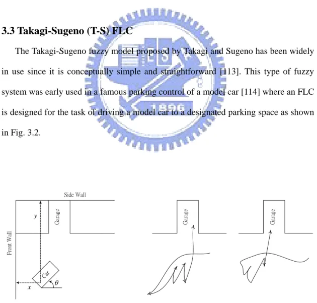
3.3 Takagi-Sugeno (T-S) FLC……....…..………...……….44

4. Speaker Adaptation Based on MAP Using a Fuzzy Controller..……...……...49

4.1 FCMAP Adaptation…………..…………..….………...……….51

4.2 Experiments…………..….………...………..…….……55

4.2.1 Database and Experiment Design………...….………...………55

4.2.2 Experiment Results………….….…..…………...………...58

5.1 FLC-VFS Adaptation.….………...………..…….……69

5.2 Experiments…………..….………...………..…….……73

5.2.1 Database and Experiment Design………….….………...………73

5.2.2 Experimental Results…………..………...………...75

6. Incremental MLLR Speaker Adaptation by Fuzzy Logic Control………...79

6.1 Incremental MLLR Adaptation (MAP-Like Adaptation)………....………….80

6.2 FLC-MLLR Adaptation (FCMAP-Like in Form)...………...85

6.3 Experiments…………..….………...………..…….…....90

6.3.1 Database and Experiment Design………...……....90

6.3.2 Experimental Results…………..….………..………...94

6.4 Fuzzy Mechanisms for the Context of Multiple Regression Classes…..……..98

7. Audio Event Detection Using Variable-Length Decision Windows…...…...100

7.1 Concepts of Short Timeslot Likelihood Difference (STLD)..……… .…....…101

7.2 Decision Windows Governed by an STLD-Driven FLC……..….….……….102

7.3 Experiments…………..….………...………..…….…..107

7.3.1 Experiment Designs…….…………..………..…………...………..107

7.3.2 Experiment Results…………....…..………...……….107

8. Conclusions and Future Works…..….……..……...………113

8.1 HMM Speaker Adaptation with FLC………..…………..…….…..113

8.2 DW and GMM Adaptation with FLC………..………..…….….115

8.3 Future Developments……..……….………..…….….115

List of Figures

Fig. 1.1 Speech/Audio information processing represented by a myriad

of branches……….………....3

Fig. 1.2 The operating structure of a typical speech recognition system………...4

Fig. 1.3 Three categories of speaker adaptation techniques in speech recognition……5

Fig. 1.4 Eigenvoice-based adaptation………..…...7

Fig. 1.5 Speaker adaptation scheme………...8

Fig. 2.1 The front-end processing procedure in preparation of subsequent audio analysis………..………..………..13

Fig. 2.2 3-state HMM model for the initial sub-syllable…………..……….………...16

Fig. 2.3 6-state HMM model for the final sub-syllable (i = 1 ~ 6)……..……...…….16

Fig. 2.4 Audio event detection system……….29

Fig. 2.5 The conventional fixed-length decision window (DW)………..33

Fig. 3.1 Architecture of a typical FLC……..………...41

Fig. 3.2 Sugeno’s FLC for car parking….……..……….………44

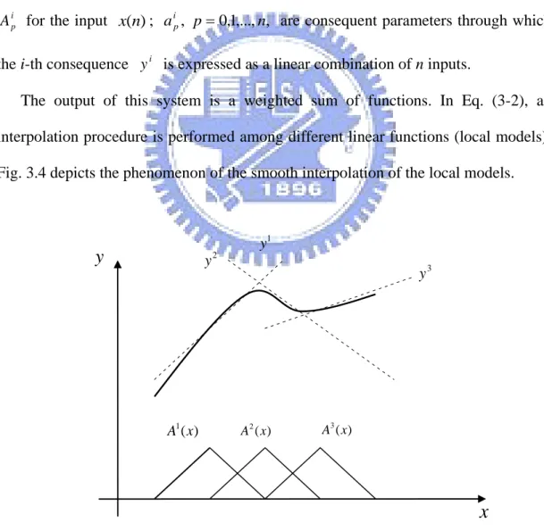
Fig. 3.3 Designs of Takagi-Sugeno (T-S) fuzzy model………..………..…...…46

Fig. 3.4 System output of T-S fuzzy model in an interpolation form...…….……..47

Fig. 4.1 Membership functions of fuzzy controllers for FCMAP adaptation…..……52

Fig. 4.2 Average recognition rates by 5 speakers using MAP with/without a fuzzy controller, using identical adaptation and testing data…..……..……...62

Fig. 4.3 Average recognition rates by 5 speakers using MAP with/without a fuzzy controller, using different adaptation and testing data…..……..……...62

Fig. 4.4 The number of adaptation utterances = 2 (MAP testing experiments)…...…63

Fig. 4.5 The number of adaptation utterances = 30 (MAP testing experiments)...…..64

Fig. 5.1 Rationale behind VFS adaptation………..……….67

Fig. 5.2 Membership functions of the FLC for FLC-VFS adaptation…….….…...69

Fig. 5.3 Average recognition rates of MAP, MAP-VFS and MAP-FLCVFS with f 20 for VFS and  30 for MAP………..76

Fig. 5.4 Numbers of adaptation utterances = 10 (VFS testing experiments)………...77

Fig. 5.5 Numbers of adaptation utterances = 100 (VFS testing experiments)……….78

Fig. 6.1 MLLR-adaptation under incremental  control (MAP-like adaptation)….82 Fig. 6.2 An investigating procedure on the role of  in incremental MLLR adaptation given a specific amount of adaptation data…….………...83

Fig. 6.3  required for holding back W_s transformation effect under various numbers of adaptation utterances………...84

Fig. 6.4 Moving toward s or Wss? And for how much?………..……….85

Fig. 6.5 Membership functions of the FLC for FLC-MLLR adaptation…..………...87

Fig. 6.6 The curve of the training values of  in FLC-MLLR adaptation…………95

Fig. 6.7 The performance curves of FLC-MLLR, MAPLR and conventional MLLR in the recognition testing experiments of the different amount of adaptation data...96

Fig. 6.8 Numbers of adaptation utterances = 2 (MLLR testing experiments)……....97

Fig. 6.9 Numbers of adaptation utterances = 10 (MLLR testing experiments)....…..97

Fig. 7.1 DW with fixed-length, each covering the same number of audio frames, n, over the time span..………..…………..………100

Fig. 7.2 DWs with variable length governed by STLD (Short Timeslot Likelihood Difference) indices………...102

Fig. 7.3 Membership functions of the STLD-driven FLC………..…………...104

Fig. 7.4 Living room audio event detection………..….111

Fig. 7.5 Parking lot audio event detection………..…112

List of Tables

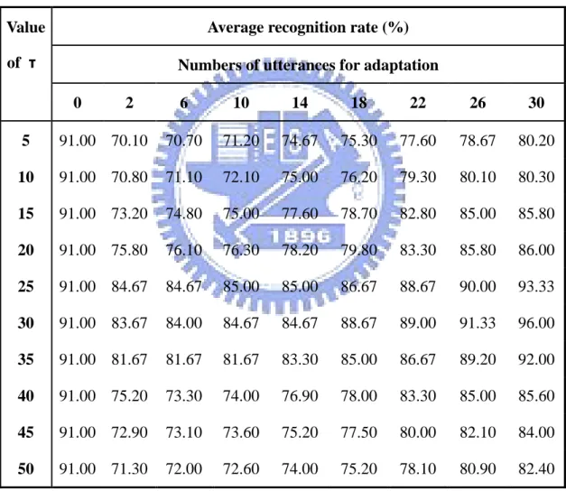
Table 1.1 A comparison between audio and visual media..……….………...2 Table 4.1 Average recognition rates (%) of the conventional MAP with

various τ ..………..60 Table 4.2 Recognition rates (%) of FCMAP and MAP (with a fixed τ

of 25 or 30)………....61 Table 5.1 Average recognition rates (%) by conventional MAP-VFS adaptation

with various f………..………..75 Table 6.1  inclination w.r.t. the variation in the quantity of adaptation data

in pursuit of recognition rate above baseline………..…….……..…………82 Table 7.1 Event detection by an FLC-regulated DW, using only LPC feature…..…109 Table 7.2 Event detection by fixed-length DW, using only LPC feature….……….109 Table 7.3 Event detection by an FLC-regulated DW, using only LPCC feature...110 Table 7.4 Event detection by fixed-length DW, using only LPCC feature..….…….110 Table 7.5 Event detection by an FLC-regulated DW, using only MFCC feature.….110 Table 7.6 Event detection by fixed-length DW, using only MFCC feature……..….111

Chapter 1

Introduction

Intelligent human-machine interaction stresses the use of vocal and visual

information as the communicating media such that the machines could interact with

people just the same as people do with one another. For the visual part, the

information process is afferent and the machine needs such device as CCD camera for

taking pictures or video sequences as the visual input from which the configuration of

the surroundings and even the status/situation reflected by the context have to be

figured out such that the machine is claimed to be able to SEE. Computer vision is the

discipline taking care of this portion of the job [1, 2].

However, the process of auditory information is both afferent and efferent. The

machine would require the microphone and recorder as the input devices for

collecting audio streams on which analysis is to be performed so that speech can be

recognized, speaker can be identified and types of audio events can be categorized,

etc; the machine also needs the synthesizer and speaker as the output devices for vocal

reactions to the people. Interestingly enough, as a counterpart of computer vision,

there is no such discipline as of “computer audition” in the realm of audio processing.

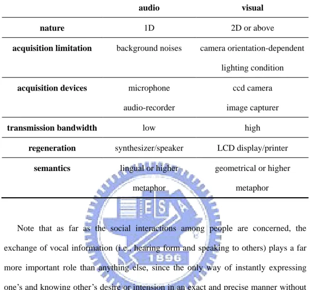
From the standpoint of signal processing, a comparison between the two media is

Table 1.1. A comparison between audio and visual media.

audio visual

nature 1D 2D or above

acquisition limitation background noises camera orientation-dependent lighting condition

acquisition devices microphone audio-recorder

ccd camera

image capturer

transmission bandwidth low high

regeneration synthesizer/speaker LCD display/printer

semantics lingual or higher

metaphor

geometrical or higher

metaphor

Note that as far as the social interactions among people are concerned, the

exchange of vocal information (i.e., hearing form and speaking to others) plays a far

more important role than anything else, since the only way of instantly expressing

one’s and knowing other’s desire or intension in an exact and precise manner without

ambiguity is through the exercise of conversation. This is true for the kids in the

preschool, as well as for various professionals in their serious careers.

The subjects in this dissertation concerns the computing techniques involved in

the process of vocal information rather than visual one, specifically speaker

adaptation schemes associated with MAP, VFS and MLLR, and audio event detection

with variable decision window, which are to be briefed in the following sections.

1.1 Scope of the Dissertation

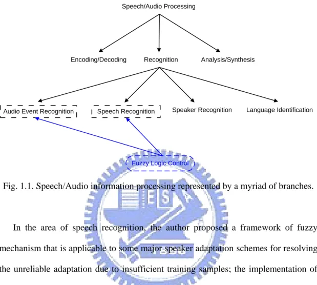
branches including, but not limited to, those shown in Fig. 1.1.

Fuzzy Logic Control Speech/Audio Processing

Encoding/Decoding Recognition Analysis/Synthesis

Speech Recognition Speaker Recognition Language Identification Audio Event Recognition

Fig. 1.1. Speech/Audio information processing represented by a myriad of branches.

In the area of speech recognition, the author proposed a framework of fuzzy

mechanism that is applicable to some major speaker adaptation schemes for resolving

the unreliable adaptation due to insufficient training samples; the implementation of

which, a series of fuzzy logic controllers embedded in MAP, VFS and MLLR

adaptations, has proven themselves by achieving far superior recognition rate at

extreme adverse conditions.

The same framework is also applied to the detection of female screaming against

different degree of background interferences, where the width of decision window

scanning through the input audio stream was adjusted by a context-driven fuzzy logic

controller.

1.2 Speaker Adaptation

and, with the ever growing maturity, have found more and more applications in

current daily life [4]. Nevertheless, the recognition performance of all speech

recognition systems ever built is undeniably inferior to a human listener as already

pointed out in [5].

Fig. 1.2. The operating structure of a typical speech recognition system.

Fig. 1.2 depicts the operating structure of a typical speech recognition system for

capturing specific short phrases or primitive statements only. Note that during the

operation any disturbances causing a mismatch between the pre-established reference

templates and the testing template would compromise the recognition performance

and the sources of disturbances may include

 speech from speakers strange to the system

 speech from speaker known to the system, only in poor “vocal shape”  various interferences in the background

 channel distortion induced in the acquisition process and so forth.

Countermeasures can be taken in two aspects:

Pre-processing -Framing -Pre-emphasis -Hamming window Signal input Feature extraction Reference templates Testing template Training Template matching Recognized result

(1) Signal filtering and normalization are deployed so that the operating condition is

in as much alignment with the referential condition as could be done.

(2) Internal tuning of the referential settings is undertaken so that the system adapts

toward the actual operating environment when new speakers appear.

Techniques in the first category work at the level of signal processing, and are

referred to as speech enhancement or feature-based adaptation through which noises

adhered to the signals are removed to make the speech signals as clean and thus

resemble to reference templates as possible. The cepstral mean normalization (CMN,

or cepstral mean subtraction CMS) [6] and signal bias removal (SBR) [7] fall into this

category too and are popular for their simplicity and effectiveness.

Approaches in the second category use sample utterances collected from the new

speaker (the end-user of the system) for adapting the system internal parameter

settings of the pre-established speech model. Consequently, they are referred to as

model-based adaptation or speaker adaptation.

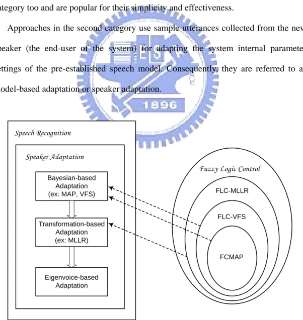
Speech Recognition Speaker Adaptation Bayesian-based Adaptation (ex: MAP, VFS) Transformation-based Adaptation (ex: MLLR) Eigenvoice-based Adaptation

Fuzzy Logic Control

FLC-VFS

FCMAP FLC-MLLR

Fig. 1.3 reveals the chronological development of the three major speaker

adaptation schemes. MAP adaptation, appearing around 1991 and the representative

of Bayesian-based adaptation, works better than the ML (maximum likelihood)

estimate of the adaptation by taking into account the information of prior means of the

model. By the nature of MAP computation, in the speech model only the portions

associated with the adaptation samples get updated, for which case VFS scheme came

into the play as a supplement to MAP by extending the coverage of adaptation in the

model space. The MAP-VFS adaptation in general offers more satisfaction in

recognition performance than MAP alone given the same adaptation data. MLLR

adaptation first appeared in 1995 and became the representative of

transformation-based adaptation, where linear regression was employed to derive the

transformation matrix using ML-estimate. Note that through the transformation by

matrix multiplication, the entire model space is adapted at one time despite the fact

that the sample utterances might convey very limited information for adaptation. In a

sense, MLLR adaptation provides with an overall but somewhat coarser speech model

adaptation, in contrast to MAP adaptation which brings about a local and yet specific

effects of adaptation, given the same adaptation samples.

One thing that is common to both MAP and MLLR is that the quality of

adaptation depends on the amount and adequacy of the adaptation samples: the more

the samples, the better the adaptation quality which in turn determines the recognition

performance. When the adaptation utterances from a new speaker are insufficient, the

effects of either MAP or MLLR adaptation would be questionable: the recognition

rate of which would fall below the baseline, i.e., worse than no adaptation at all as

shown by the author’s experiments [8, 9].

Eigenvoice-based adaptation [10-20] is a relatively young member in the speaker

speaker-clustering-based adaptation where a speaker dependent (SD) speech model is

established for every member in a group of speakers, from which feature vectors

called as eigenvoices are extracted through PCA for building the eigenvoice speech

model. The adaptation to the speech model (an eigenvoice vector space) then can be

undertaken when adaptation data is available, as shown in Fig. 1.4.

. . . . . . . . . . . . . . PCA ._. . ML Estimate . . . Adaptation Data . . . S pe ak er 1 S pe ak er N Speaker Adapted Model SD models SA model unused weights 11  11 12  12 13  13 1 N  N1 2 N  N2 3 N  _N3 1  2  3 

To summarize, speaker adaptation is a process that turn speaker-independent (SI)

speech models into speaker-adapted (SA) ones, as is clearly seen in Fig. 1.5.

SI models speech recognition system

SI models

speech recognition system

SA models shipping

from manufacturer to end user

adaptation data from end users

adaptation process

Fig. 1.5. Speaker adaptation scheme.

To ensure the quality of the adaptation at the scarcity of adaptation samples, the

author proposes a general framework for enhancing MAP, VFS and MLLR adaptation,

and the resultant implementations are named as FCMAP, FLC-VFS and FLC-MLLR

respectively where FLC stands for fuzzy logic control, indicating the underlying fuzzy

mechanism incorporated in the general system architecture.

1.3 Audio Event Detection

Conventional security, surveillance or remote homecare systems rely heavily, if

not exclusively, on the visual information (i.e. data captured by video camera) for

detecting specific events in considerations [21-24] through the use of motion tracking-

analysis techniques. The similar development is also seen in the field of multimedia

retrieval and indexing applications, where video information is the major concern and

detecting certain specific shot in a video sequence [25-27]. Depending solely on

visual data as the basis for capturing status/situation development in the context

inevitably would be confronted by the limitations inherent in the image acquiring

process:

 Video camera is an oriented-sighting device and views lying beyond the camera’s visual angle are therefore “unseen”.

 When the scene is in the darkness or over exposure, activities taking place wherein would become “unseen”.

 The scenario like two gangsters threatening of killing each other right in front of the video camera, both with smiling on the faces, is in fact “unaware of” through

“clearly seen”.

Note that in all these circumstances, acoustic data can act as a complementary source

of information for reflecting the auditory aspect of the reality in the context. A further

thought in that almost all living creatures that move around in their habitats are

equipped with organs for both visual and aural perception would remind us that any

security, surveillance or remote homecare system dismissing the use of audio

information is effectively a crippled one. And in fact species that can “hear” much

better that they can “see” are more than one would have expected; scotopic animals,

oceanic mammals and, of course, the moles are only a small group of examples of all.

As a result, audio event detection has been getting a lot more attentions in recent years,

and fundamental issues include

(1) Categorization of various kinds of sounds that are to be encountered in daily life,

of which the sources may be

 artificial: gun shots [28], door opening/closing and glass breaking [29].

 human activities: coughing [30], voices under different emotions [31], crying, talking, walking and running [32], female screaming to be addressed in this

dissertation (Chap. 7).

 nature: wildlife activities [33] and ordinary or catastrophic phenomena [34]. Note that the entities of the categorization are not limited to the above three and in

each category good and interesting subjects to be explored are virtually unlimited;

“detecting a tiny mouse blowing wind one mile away”, for instance, borrowing from the dialog in an old movie in the early 80’s “Blue Thunder” is just one if the

author is allowed.

(2) Internal representation and modeling of a designated type of sound, in order to be

differentiated from other sounds and the background acoustics as were done in [32]

and [28], where multi-level or hierarchical tree are utilized for more elaborated

audio representation of several human activities and different types of gunshots,

respectively.

(3) Representation and modeling of the background acoustics against which the

compasison can be done for audio event detection, as was done in [35] for

background noise analysis, and in [36] for online adaptation in background

modeling where the idea of acoustic background modeling is translated from a

precedent counterpart in video background modeling [37].

A typical audio event detection process starts with receiving a stream of audio

frames coming in the system at regular time intervals, on which analysis is to be

performed every time a fixed number of frames are collected (or equivalently an

elapse of a pre-determined time span called decision window, DW) so as to decide if

the designated audio event has occurred or not. The author proposes a variable-length

decision window of which the window length is governed by a fuzzy mechanism for

eliminating the deficiency suffered by the fixed-length DW approaches, as to be

detailed in Chap. 7.

automatic speech recognition based on hidden Markov models for Mandarin is given,

together with the mathematic backgrounds for the two speaker adaptation techniques

in popular use: MAP-VFS composite and MLLR. Also described in Chap. 2 is audio

event detection based on Gaussian mixture models. In Chap. 3, a general framework

of fuzzy logic control is described, where the problem formulation by fuzzification,

the establishment of fuzzy rule base and inference mechanism, and the defuzzification

for final quantitative outputs are provided.

The main theme of this dissertation concerns the enhancement of extant speaker

adaptation schemes by additional tuning according to the availability of adaptation

data and of audio event detection by scanning the audio stream with a variable-sized

decision window, both being govern by a general fuzzy mechanism; the formulation

and implementations of which are explained respectively in chapters 4, 5, 6 and 7.

Chapter 2

Overview on Speech Recognition and Audio

Event Detection

In the realm of man-machine interactions, audio processing no doubt receives far

less attention than it deserves when compared to the resources/efforts invested in its

counterpart of video processing. It has been so for over decades despite the fact that

for thousands of years in human history instant and precise communications among

individuals were mostly realized via the auditory channels: speak and listen (imagine

the age before the creation of characters in ancient civilization).

Though the ability to understand what others are talking about is indispensable in

social interactions, the auditory perceptual skill of differentiating one kind of sound

from others that may be heard in one’s living surroundings is far more important and

crucial; for instance, being able to tell other’s “HELLO” from the noises due to a

vehicle’s hard break, a gunshot from an explosion, a duck’s quack from a goose’s

honk and the Spanish from the Italian without really understanding both languages etc.

could be live-saving or at least useful or even amusing in one’s daily life.

Paradoxically enough, the development in audio process evolved in the opposite order:

speech recognition was addressed far ahead of audio event detection which was not

until recent years did it become visible on the stage.

Before the analysis on the audio information could commence, a pre-processing

on the input audio signals is generally required for extracting acoustic features in

preparation of any particular application under consideration, and in the case of this

several major steps in the front-end processing is briefly explained as follows [38,

39]:

Analog to digital conversion (A/D conversion)

Pre-emphasis Feature extraction

Framing processing Speech signals input Hamming windowing Feature vector output

Fig. 2.1. The front-end processing procedure in preparation of subsequent audio

analysis.

(1) A/D conversion:

The analog input data is converted into digital forms by sampling and A/D

conversion.

(2) Pre-emphasis:

Components in the high-frequency band are enhanced.

(3) Framing:

Samples of audio data are divided into frames, each consisting of a

pre-determined and same number of samples.

(4) Hamming windowing:

(5) Feature extraction:

From each frame, various parameters are extracted and a feature vector

representing acoustic characteristics of the audio input in the associated time

period is thus derived.

For the purpose of speech recognition and human voice related application, linear

predictive coefficient (LPC) parameters, LPC cepstrum (LPCC) parameters and mel

frequency cepstral coefficient (MFCC) parameters are the three most frequently seen

in practice, and are employed in the author’s research.

In this chapter, theoretical backgrounds for two fundamental technical issues in

speech recognition, namely HMM speech modeling and speaker adaptation, will be

given; also given in the final are certain primary issues pertaining to audio event

detection.

2.1 HMM Speech Modeling

The modeling of speech patterns can be implemented in the form of neural

networks (NN, [40-42]), by using support vector machine (SVM, [43, 44]) or by using

hidden Markov models (HMM) which to the author’s knowledge is by far the most

popular and widely used one.

2.1.1 HMM and Mandarin Syllable Modeling

HMM is basically a stochastic process operating on an underlying Markov chain

of a finite number of states and the same number of random functions: at any given

instance of time, the process stays at a certain state and the random function

associated with the current state determines what the next state will be. Such issues as

how an HMM is to be cast into a model for certain specific applications and how the

probability transition matrix is used to describe the probability of going from one state

to the other states, which in effect defines the Markov chain at work. The applications

of HMM to speech recognition can be found in many references. [48-51] are some of

the examples. The work by C. H. Lin et al. [50] is particularly note worthy, where a

framework for the recognition of syllables was established and later became a widely

accepted standard in the modeling of Mandarin syllables with tones. According to

which each Mandarin syllable consists of an initial part and a final ending part, each

being called as a sub-syllable. The HMM modeling of Mandarin syllables assumes

that the initial part is right dependent on the beginning phone of the following final

part and the final part is context independent. A Mandarin utterance may contain one

to several syllables; the HMM of an utterance thus includes HMMs of the constituent

syllables. In the actual implementation of the author’s work, the HMM of a syllable

consists of an HMM of 3 states for the initial part and an HMM of 6 states for the

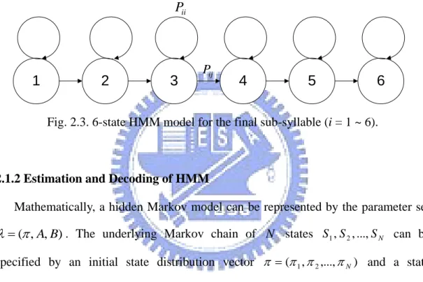
final part, and in total there are 440 states for all Mandarin sub-syllables. The HMM

modeling of the initial sub-syllable in 3 states and the final sub-syllable in 6 states are

respectively depicted in Fig. 2.2 and Fig. 2.3, where each circle represents a state and

ij

P represents the probability density function concerning the transition from state i to

state j. The HMM model employed in the author’s research is referred to as

left-to-right model since only left-to-right transitions are allowed; i.e. the transition

from each state is limited to only two alternatives: either moving toward the

1

2

3

Fig. 2.2. 3-state HMM model for the initial sub-syllable.

5

4

1

2

3

6

Fig. 2.3. 6-state HMM model for the final sub-syllable (i = 1 ~ 6).

2.1.2 Estimation and Decoding of HMM

Mathematically, a hidden Markov model can be represented by the parameter set

) , , ( A B

 . The underlying Markov chain of N states S1,S2,...,SN can be

specified by an initial state distribution vector  (1,2,...,N) and a state

transition probability matrix A





S at time t 0 and a is the state transition probability of going from state _ij Si

to state S . Moreover, if the observations composed of _j M discrete symbols

M o o

o₁, ₂,..., are considered, the finite set of probability distributions





B j( )|1  ,1  with bj(q) being the probability of observing o q

given the state S , represents the random processes associated with the states. _j

number of observation symbols M also should be taken into account besides

specifying the parameters , A and B.

In order to acquire an efficient estimation of HMM model during the training

phase and an optimal decoding procedure of the estimated HMM model during the

recognition phase, three problems need to be taken care of [51]:

(1) If the observation sequence O 





) | (O 

p is to be evaluated then?

(2) If an HMM model and an observation sequence are known, how the optimal (the

most likely) state sequence in the model that produces the observation is to be

decide?

(3) If a model and a set of observations are given, how the model parameter set

) , , ( A B

 to maximize p(O|) is to be estimated?

For the first problem, some methods such as the forward recursive algorithm and

backward recursive algorithm have been proven to be efficient [52]. For the third

problem, the Baum-Welch method [45-47] is proposed to offer a local maximum

solution although the computation for an explicit solution of the model  is difficult.

For the second problem, the Viterbi algorithm proposed in [53] has been proven to

be an effective one for acquiring an optimal state sequence. The score function _t(i)

is defined as in Eq. (2-1), given the observation sequence O





) | ,..., , , ,..., , ( max ) ( _{1 2 1 2} ,..., ,₂ 1   t i T s s s t i P s s s S o o o t   , (2-1)

where _t(i) has the largest probability at time t and at state S_i.

) (

1 i

t

 is computed as follows using t(i) by induction,

) ( ] ) ( max [ ) ( ₁ 1    t ij j t i t j  i a b o  . (2-2) This iterative procedure is essentially a dynamic programming and the state sequence

that has the maximum likelihood of generating the given observation sequence will be

searched if one keep track of all the states which maximize Eq. (2-1). An array t( j)

is used to store the predecessor state of the state j at t . The steps of the Viterbi

algorithm are as follows

(1) Initialization , 1 ), ( ) ( 1 1 i ibi o iN  (2-3) , 1 , 0 ) ( 1 j   j N  (2-4) (2) Recursion , 1 ), ( ] ) ( [ max ) ( ₁ 1 i a b o j N j _{t ij j t} N i t  _      (2-5) , 1 ], ) ( [ arg ) ( 1 1 N j a i j t ij N i t         (2-6) (3) End )], ( [ max 1 * i p _T N i    (2-7) )], ( [ arg 1 * i s _T N i T     (2-8) (4) Back-tracing 1 ,..., 2 , 1 ), ( *₁ *     t T T s s_t _{t t} . (2-9) During the recursive step of this algorithm, the optimal sequence of states is obtained

eventually.

2.2 Speaker Adaptation

Automatic speech recognition systems generally can be classified either as

speaker-independent type (SI) or speaker-dependent type (SD), depending on how

speech samples are colleted during system construction. An SI system typically

collects speech samples from an as large population of speakers as possible, whereas a

speaker. In general, a well-trained SD model achieves better performance than an SI

model on recognizing the speech of a specific speaker. However, when the amount of

training data available to acquire the SD model is not sufficient, such superiority

would no longer exist. This is where speaker-adaptive techniques (SA), sometimes

referred to as model-based adaptation techniques, get in to play, which would adapt a

full SI model into an SD one and achieves SD-like performance, requiring only a

small fraction of the speaker-specific training data. When a new speaker uses such an

adaptive system, the parameters of the HMMs are updated by speech data obtained

from this speaker. By speaker adaptation, the recognition performance can be

significantly improved for outlier speakers such as non-native speakers or others not

well represented in the SI training set.

Generally speaking, the operation for speaker adaptation can be carried out in

either supervised mode or in unsupervised mode respectively, depending on if the

transcription of the speaker-specific adaptation data has been known or not before

performing the adaptation procedure [54]; the speaker adaptation is said to operate in

batch mode if all adaptation data acquired from a new speaker is fed into the system

before the final adapted system is produced and then put to work, or incremental

mode if the adaptation data is continually fed for adaptation while the system is

already at work [54].

Currently there mainly three categories of speaker adaptation techniques:

(1) Maximum a posteriori (MAP) adaptation, representative of Bayesian-based

adaptation.

(2) Maximum likelihood linear regression (MLLR) adaptation, representative of

transformation-based adaptation.

(3) Eigenvoice adaptation.

are the most commonly used techniques for speaker adaptation, and practically are

still seen working in almost all speech recognition systems nowadays. The

schemes of the three speaker adaptation will be described in the following

subsections.

2.2.1 Bayesian-based Adaptation

In early 90s, Lee, Lin and Juang reported speaker adaptation for an HMM with

parameters of continuous density (CDHMM) [55], in which the parameter estimation

was accomplished by segmental k-means algorithm which was developed in their

earlier researches for HMM parameter estimation/training [56, 57]. In these works,

speaker adaptation of CDHMM parameters is formulated as a Bayesian learning

procedure, where prior information were involved in the computation of Bayes

theorem P(|O) where  is the model parameters and O is the sequence of observations. On this basis, Gauvain and Lee then released in 94 the MAP adaptation

by maximum a posteriori estimate of the HMM parameters [58]. MAP adaptation is

thus Bayesian-based and offers a framework of incorporating newly acquired

speaker-specific data into the existing models.

Assume that the CDHMM parameters are characterized by the parameter vector





 , ,

 , where wik, ik and ik are the mixture gain, mean vector and

covariance matrix of the k-th mixture component from the i-th state, respectively. The

parameter vector  is a random vector. A prior knowledge about the random vector is available and characterized by a prior probability density function p() where  is to be determined as the input sequence is observed. Let Y (y₁,...,y_T) be a given set of T observations. The MAP estimate for  is defined as

)]. | ( [ max arg p Y MAP     (2-10)

Then the MAP estimate for  is obtained by solving . 0 ) ,..., , | ( _{1 2}    T y y y p   (2-11) By using Bayes theorem,

. ) , . . . , , ( ) ( ) | , . . . , , ( ) , . . . , , | ( ) | ( 2 1 2 1 2 1 T T T y y y p p y y y p y y y p Y p       (2-12)

Then Eq. (2-10) can be rewritten as follows:

 a r gm a x[ ( |) () ] .

 p Y p

M A P (2-13)

To accomplish the estimation of the model parameter vector , the well-established segmental k-means algorithm can be used, and the execution is done in an iterative

process as follows:

(1) Obtain the optimal state segmentation of a given observation sequence Y, based on

a given model, i.e.,

) ( ) | , ( max arg ˆ P Y s  P  s s  , (2-14) where s(s₀,s₁,...,s_t,...,s_T)is a state sequence.

(2) Based on the optimal state sequence sˆ , find the MAP estimate

 a r gm a x ( ,ˆ|) ()

 P Y s P





. (2-15) (3) Iterates from (1) until some predefined equilibrium is reached.

Assume that the mean  is random with a prior distribution P₀() and the variance 2 is known and fixed, then the conjugate prior [59, 60] for  is also a Gaussian distribution with mean  and variance ~2, as already shown in [61]. And if the conjugate prior for the mean  is substituted into Eq. (2-13), the MAP estimate for the adapted parameter  as derived in [61] would appear as a weighted average of the prior mean  and the mean of the adaptation observation data yk:

       ˆ ₂ ~2_{~2 2} 2 _~2        k k k k k N y N N , (2-16)

where N_k is the total number of training samples observed for the corresponding

recognition unit with the k-th Gaussian and yk is the sample mean with the k-th

Gaussian.

Let  2/~2 and the prior mean  be replaced by the mean parameter of the initial model with the k-th Gaussian, _k, Eq. (2-16) could be reformed as

_k k k k k k N y N N          ˆ , (2-17) where  is a parameter which gives the bias between the maximum likelihood estimate of the mean from the data and the prior mean. That is,  is a prior density parameter that controls the balance between the prior knowledge and the adaptation

data.

Note that, however, the data available for adaptation is often quite limited and

most likely could cover a small portion of speech patterns in HMMs, which implies

that many HMM parameters will not be adjusted by the nature of Bayesian-based

adaptation. As a result, vector field smoothing (VFS) was proposed as a supplement

for broadening the extent of adaptation in the HMM parameter vector space [62-65].

The rationale behind VFS adaptation is that, by exploiting the spatial coherence of

vector distributions in HMM, the unadapted HMM parameter vector might be

“purposely” adjusted in accordance with the MAP adapted vectors nearby.

To be specific, consider an unadjusted parameter vector _j and k of MAP adapted vectors ˆk’s with initial counterparts k’s lying in the vicinity of j in the

HMM vector space. The amount of MAP adaptation to k is referred to as the

transfer vector k,

k k

k  

  ˆ  . (2-18) Given the adapted vectors around, how much adaptation to _j should be

expected? A weighted average of _k’s as shown in Eq. (2-19) would be a quite natural choice. j j N k k j j N k k k j j        





) ( j

N indicates the set of K-nearest neighbor mean vectors, k’s, to j; k

j,

 represents the weighting coefficient determined by the distance d_j,k

between _j and k, and

f denotes the weight control parameter.

A typical VFS adaptation thus comprises three steps:

(1) transfer vectors calculation for all MAP adapted parameter vectors by Eq. (2-18),

(2) interpolation of transfer vectors for adapting the unadjusted vector by Eq. (2-19),

(3) smoothing.

The composite of MAP-VFS adaptation has been proven to be more robust than

MAP adaptation in recognition performance when given the same limited amount of

adaptation data. Still there are rooms for MAP-VFS enhancement when the quality of

MAP adaptation is in question, which is an issue to be addressed in Chap. 5.

2.2.2 Transformation-based Adaptation

In the transformation-based model adaptation, certain appropriate transformations

have to be derived from a set of adaptation utterances acquired from a new speaker

cepstral bias for model adaptation is the simplest form of transformation, which is

easy to estimate and perform, as was done in [66]. Usually, adding a bias alone could

not take care of the variations in test environments or among different speakers. An

affine transformation (linear transformation) over HMM parameters in general offers

a more appropriate model and there have been numerous adaptation schemes using

affine transformations. In the work by Leggetter et al. [67], MLLR adaptation was

firstly proposed under the framework of affine transformation, which has become

quite popular and successful for its rapid adaptation. However, it is necessary to have

sufficient adaptation data to ensure the estimate of the MLLR transformation, and

various solutions have been suggested for further reinforcement. For instance, instead

of using the maximum likelihood (ML) estimate in the MLLR scheme, the maximum

a posteriori estimate is used to estimate the transformation parameters by maximizing

the posterior density [68, 69]. In addition, it is suggested in [70, 71] that a prior

distribution for calculating the mean transformation matrix parameters is used, which

is generally dubbed as the MAPLR technique. Besides using the estimate of MAP

style for acquiring transformation parameters, an alternative using a variant of the

Expectation-Maximization (E-M) algorithm [72] to optimize a discounted likelihood

criterion, the so-called discounted likelihood estimation, was proposed in [73].

Theoretical formulations of classic transformation-based adaptation schemes, MLLR

and MAPLR, are briefly described as follows.

Under the framework of the transformation-based speaker adaptation, it generally

starts with a set of SI HMMs,  to which certain transformation F with _

parameters  derived from adaptation data, Y, of a new speaker is to be applied such that the transformed model F_() would recognize the incoming speech better than

usually assumed to be fixed and then be estimated via statistical measures under

specific criteria such as ML or MAP, as were done in [67] and [70] respectively.

MLLR makes use of the simplicity of ML criterion, which states that the

transformed model ˆML should maximize the likelihood of the adaptation data

) , | (Y  p , i.e. ˆ a r gm a x ( | ,)    p Y ML . (2-20)

Consider the Gaussian mean vector of the model at state s, s, and the associated

affine transformation action as follows

, ˆ_s  A_s _s b_s

 (2-21) which sometimes is written as

, ˆ_s W_s _s

   (2-22) and s is the extended mean vector in the form

, ]' , , , [ 1 sn s s       (2-23) where  is the offset term of the regression, usually being set as 1.

The transformation matrix Ws is to be estimated such that the likelihood of the

adaptation data is maximized, for which a closed form solution is available in [67] by

solving the following equation,

, ) ( ) ( 1 1 ' 1 1 1 ' 1





 is the total occupation probability for the state s at time _r t given the

observation vectors of adaptation data ot at time t;

1 

s_r is the covariance matrix of the output probability distribution, and

R is the number of states.

Apart from MLLR, Chesta et al. [70] suggests that the prior density can be taken

maximum a posteriori criterion: ), , | ( max arg ˆ_MAP  p Y    (2-25)

which is proportional to argmax ( |, ) ().

 p Y  p According to this criterion, the

maximum a posterior linear regression (MAPLR) technique for adaptation is thus

derived, where the transformation matrix W_s appears in the form of p(p1) linear equations as follows [70]

, 1 1 1 2 1 2 1 ) ( ) , ( 2 1 2 1 ) , ( , 1 1 1 1 1 1 1 1 1 1 1 1                                  

  

 



 is the probability of the mixture m in state n at time t, given the observation o(t), and

i

 is the i component of the mean vectorth nm.

Note that Rnm is the precision matrix and M ,  and  are hyperparameter

matrices associated with the prior density. Solving the system of equations in Eq.

(2-26) for Ws is obviously much more time-consuming than standard MLLR due to

the use of additional hyperparameters









A fuzzy control mechanism reinforced MLLR, called FLC-MLLR, will be

presented in this dissertation to perform at a much lower computing cost than

MAPLR and still be able to ensure the quality of MLLR adaptation when

2.2.3 Speaker-clustering-based Adaptation

The basic idea of the speaker-clustering-based adaptation is that a number of

speaker clusters can be built up in advance, and the model of the current speaker is

then represented as an interpolated form of the weighted sum of the speaker clusters.

Such a speaker-clustering-based adaptation is also called as speaker-space-based

adaptation. Mathematically, the estimated parameters of the sets of cluster models

form the axes of speaker spaces and by estimating an appropriate point for the speaker

in the speaker space, the mean vectors for the speaker is then determined. The

eigenvoice approach can be regarded as the generalization of speaker-clustering

adaptation techniques.

R. Kuhn, et al. [10] firstly proposed the eigenvoice adaptation where a priori

knowledge concerning the variations among all training speakers was represented as

the set of SD model parameters in the form of eigenvectors named eigenvoices; a new

speaker model was then expressed as the linear combination of the set of eigenvoices.

By the eigenvoice approach, the number of parameters required to be estimated would

be reduced greatly but still capable of retaining the overall system characteristics to

capture the variance between speakers.

Typically, the eigenvoice approach needs to take care of two things, namely

eigenvoice construction and coefficient estimation. In the eigenvoice construction

phase, referring to Fig. 1.4, a set of N well-trained SD models must be established

first. Then, the model parameters of each SD model are “vectorized”, forming a set of

N “supervectors”. Space dimension reduction techniques, such as principal

components analysis (PCA), are then applied to the set of N supervectors to obtain N

eigenvectors with dimension D, also called as “eigenvoices”. In general, only the first

K eigenvoices are kept which are significant as they possess most information from

Finally, by these K eigenvoices, an accurate speaker space “K-space” will be spanned

and acquired. In the coefficient estimation phase, adaptation is then performed using

the maximum likelihood eigen-decomposition (MLED) algorithm proposed in [10],

which estimates a set of weights to find a weighted combination of eigenvoices.

Following the eigenvoice representation, the eigenvoice-versioned MLLR and

MAPLR adaptation have been reported in [11] and [12] respectively where effective

hybrids of MLLR-/MAPLR-eigenvoice adaptation are conceived. For the time being,

the eigenvoice-based approach has received intensive attentions and various

extensions of eigenvoice adaptation have been developed [13-20].

2.3 Audio Event Detection

The audio event detection system is designed for picking up a designated acoustic

phenomenon when it appears in a certain acoustic background, and consequently the

operations basically involve the comparison of the input audio signals against two

acoustic models (the singular and the normal) and the decision about whether an

audio event has occurred or not. Fig. 2.4 shows the architecture of a typical audio

event detection system associated with two sound models where the input audio

stream is segmented into the frame sequence, from which acoustic features are to be

extracted for estimating the likelihood scores of both the normal and the singular

situation via the classifier operation. When collecting the likelihood estimates to the

Feature Extraction

Likelihood scores for the normal class Frame 1

Likelihood scores for the singular class

Feature Extraction

Likelihood scores for the normal class Frame 2

Likelihood scores for the singular class

Feature Extraction

Likelihood scores for the normal class Frame n

Likelihood scores for the singular class

Input audio frames

.

.

.

.

.

.

.

.

.

.

.

.

.

.

.

.

.

GMM classifiers (Event models)

Pre-established database for the normal class

Database for the singular class DW: covering n feature vectors

Fig. 2.4. Audio event detection system.

For constructing such a system as in Fig. 2.4, several issues have to be resolved.  acoustic features to be extracted:

LPC, LPCC and MFCC, for example, are good candidates to be considered.  acoustic/sound models:

In what kind of representations and how the model parameters are to be

determined are the primary concerns. For the representation, alternatives like GMM

[75], HMM [76] or Bayesian network [77] are available. GMM is in relatively

density distributions [78]; GMM is also frequently seen employed in the field of

speaker identification for its capacity in categorizing voice patterns.  the criteria for decision making:

How the likelihood estimates are to be calculated and accumulated, how

frequently the decision should be made, and the possibility of making decision not

at regular time intervals but being situation driven are all interesting subjects to be

explored.

2.3.1 GMM Models and Classifiers

In this dissertation, GMM models are adopted in the development of an audio

event detection system for female screaming in the contexts of office space, parking

lot and living room. The setting up of models during the training phase and the

operation of the GMM classifier during the recognition phase are described in the

following.

2.3.1.1 GMMs Establishment

Mathematically, a GMM is a weighted sum of M Gaussians, denoted as







To determine the GMM model parameters for a certain sound class, the E-M

algorithm as suggested in [72] is readily applicable. It is noted that before running the

E-M algorithm, a crucial job is to initialize the model first, i.e., to assign starting

values to the parameters, which can be realized by a binary splitting vector

quantization algorithm [79]. With the initial model parameter settings, the E-M

adjusting the initial model parameters; specifically, the expectation and the

maximization steps in the E-M process are repeated so that the parameter set





 

 of the GMM converges to an equilibrium state. The

E-M algorithm implemented in the system to establish a GMM model, given a set of

acoustic feature vectors {x_n |n1,2,...,N}, is detailed below:

(1)  initialization is performed by a binary splitting vector quantization algorithm [79]; _i is in diagonal form for computational consideration; M is determined by the Bayesian Information Criterion as suggested in [80].

(2) The computation for GMM parameters is, as suggested by the name E-M,

basically an iterative process through which GMM parameters are progressively

updated for maximizing the expectation value of the acoustic data.

REPEAT {Expectation computation:



-update for f() maximization:

1 ( | , ) 1 





