不動產評價之空間計量與地理統計 - 政大學術集成

全文

(1)國立政治大學商學院金融學系博士論文指導教授：廖四郎博士. Spatial Econometrics and Geostatistics for Real Estate 治政 Valuation. 大. 立不動產評價之空間計量與地理統計 ‧. ‧ 國. 學. n. er. io. sit. y. Nat. al. Ch. engchi. i n U. v. 研究生：陳靜宜中華民國. 一○二. 年. 七. 月.

(2) Abstract In recent years, spatial data analysis has received significant awareness and played an important role in social science because of the rapid development of Geographic Information System (GIS). Although classic statistical methods are attractive in traditional data analysis, they cannot be executed seriously for spatial data. Standard statistical techniques didn’t sufficiently deal with spatial dependence or spatial heterogeneity issues. Generally, the model-driven method and the data-driven method. 政治大 to apply spatial statistics methods including geostatistical methods (kriging and 立. are mainly the two branches of the spatial data analysis. The purpose of this paper is. cokiging), geographically weighted regression, and spatial hedonic price models to. ‧ 國. 學. real estate analysis. It seems to be completely reasonable and sufficient. The real. ‧. estate data in Taichung city (Taiwan) is used to carry out our exploration. These. sit. y. Nat. techniques give better insight in the field of real estate assessment. They can apply a. io. er. good instrument in mass appraisal and decision concerning real estate investment.. al. n. v i n Cautocorrelation, Keywords: house prices, spatial U econometrics, geostatistics, h e n g c h ispatial kriging, cokriging, geographically weighted regression. I .

(3) 摘要近年來由於地理資訊系統（GIS）的快速發展發，空間資料分析開始受到重視並在社會科學領域中逐漸扮演重要的角色。雖然一般的統計方法已在傳統資料分析上發展已久，然而它們卻不能有效地說明空間性資料，並且無法充分處理空間相依或空間異質性問題。一般而言，空間資料分析主要有兩個分派:模型導向學派與資料導向學派。本文研究目的在於應用空間統計方法合理且充分地評估房地產價值，研究方法包含地理統計(克利金和共克利金)、地理加權迴歸與空間特徵價格模型等，並且以台中市不動產資料進行實證探究。這項新的研究技術在不. 政治大. 動產評價領域中將可提供更好的解析能力，使其在評價過程中或是不動產投資決. 立. 策時，成為一個更強而有力的分析工具。. ‧ 國. 學. 關鍵字: 房價、空間自相關、空間計量學、地理統計學、克利金、共克力金、地. ‧. 理加權迴歸. n. er. io. sit. y. Nat. al. Ch. engchi. II . i n U. v.

(4) 致謝在博士論文寫作的日子裡，無論其過程如何艱辛，但由於有朋友、師長與家人的陪伴與支持，使我在這寫作過程中最終得以順利完成。首先我要感謝的是，廖四郎老師的指導，其給予我在論文的寫作上擁有相當大地發揮空間，並且在於研究方向上的提點與指正，使得本篇論文得以進行。同時也要感謝論文口試時，承蒙各位口試委員林左裕老師、林士貴老師、張光第老師、江淑玲老師與陳芬英老師不吝給予指正與建議，使得本篇論文能更加精進與完整，在此深表謝意。接著我要感謝我的同窗好友們，宏銘、信豪、俊凱、典霖，因為有你們的陪. 政治大在我失意遇挫時能重新站起堅持下去。另外，特別是宏銘在課業上的幫助與指導，立伴，讓我在隻身前往台北的日子裡增添無數的色彩與回憶，也因為有你們的支持. ‧ 國. 學. 使得在數學理論推導上得以解惑，由衷感謝。還有安琪的熱情與好客，常常帶著營養補給給我加油打氣;此外謝謝淑芳助教在求學期間的協助，使得在相關行政. ‧. 處理上得以簡要從容，感謝之情無以言喻。. sit. y. Nat. 最後，我要感謝我的家人，感謝父母辛苦的撫育與栽培，使我在求學期間能. al. er. io. 無後顧之憂，並且感謝子桓的陪伴與開導，使我在這些年，心境得以轉換與成長，. v. n. 因為有你們讓我可以順利獲得博士學位，謹將此份榮譽獻給我所感謝的每一位，在此獻上由衷的感激。. Ch. engchi. i n U. 陳靜宜謹誌於國立政治大學金融系中華民國 102 年. III .

(5) Contents Chapter1 RESEARCH MOTIVATION AND PURPOSE . 1 . Chapter 2 RELATED LITERATURE . 5 . Chapter 3 STUDY AREA DESCRIPTION . 8 . Chapter 4 GEOGRAPHICALLY WEIGHTED REGRESSION APPROACH . 15 . 4.1 Linear Regression (Global Model) . 15 . 4.2 Geographically Weighted Regression (Local Model) . 16 . 4.3 Empirical Analysis . 20 21 . 4.3.1. Results of Global (OLS) Model . 政治大. 22 . 4.3.2. Results of Local (GWR) Model . 立. 4.4 Summary . 24 . ‧ 國. 學. Chapter 5 MEASUREMENTS OF SPATIAL AUTOCORRELATION AND SPATIAL MODELS 25 25 . 5.1 Spatial Autocorrelation . ‧. 5.2 Spatial Lag Model (SLM or SAR) . sit. y. Nat. 5.3 Spatial Error Model (SEM) . io. al. n. 5.5 Summary . er. 5.4 Empirical Analysis . Ch. n U engchi. Chapter 6 GEOSTATISTICAL APPROACH 6.1. Semi-Variogram . iv. 27 27 28 34 35 36 . 6.2. Ordinary Kriging . 38 . 6.3 Cokriging . 40 . 6.4 Understanding the Dynamical Changes in House Price in the Study Area . 41 . 6.5 Predict House Price in 2012 . 42 . 6.6 Empirical Analysis . 42 . 6.7 Summary . 56 . Chapter7 CONCLUSIONS . 58 . REFERENCES . 62 . APPENDIX 1 . 66 IV . .

(6) APPENDIX 2 . 70 . APPENDIX 3 . 71 . 立. 政治大. ‧. ‧ 國. 學. n. er. io. sit. y. Nat. al. Ch. engchi. V . i n U. v.

(7) Figure 4 . Figure 1. 1 Research Organization Chart . 10 12 . Figure 3. 1 Geographic Area of Study City Figure 3. 2 Average House Price for Taichung City by Year . Figure 3. 3 Geographical Locations of the Observed House Prices in 2002 (Starting Year of Study) 13 Figure 3. 4 Geographical Locations of the Observed House Prices in 2011 (Ending Year of Study) 13 Figure 3. 5 Yearly Average House Price for Each District in the Study Area 14 . 政治大. Figure 4. 1 The Kernel with Fixed Bandwidth Figure 4. 2 The Kernel with Adaptive Bandwidth Figure 4. 3 Spatial Variation of the DCTSP Coefficient Figure 5. 1 Changes in Spatial Autocorrelation Along with the Distance . 立. 學. ‧ 國. 17 17 24 29 . ‧. Figure 5. 2 Graphical Summary of Spatial Autocorrelation Reports in 2011 (ID_0.04) 30 Figure 5. 3Moran Scatter Plot for OLS_Residue 33 Figure 5. 4Moran Scatter Plot for Lag_Residue 33 Figure 5. 5Moran Scatter Plot for Error_Residue 34 Figure 6. 1 Directional Semi-Variograms of House Prices in 2011 43 Figure 6. 2 Experimental and Fitted Semi-Variograms for Anisotropy in 2011 44 Figure 6. 3 Contour Maps Obtained through Kriging of House Prices 46 Figure 6. 4 Contour Maps Obtained through Kriging of Estimation Variance 48 Figure 6. 5 Scatter plot of Predicted (kriged) Versus Measurement House Prices 50 . n. er. io. sit. y. Nat. al. Ch. engchi. i n U. v. Figure 6. 6 Correlation between Measurement House Prices and Associated Estimation Error Figure 6. 7 Yearly Increment Value of Interpolated House Price Figure 6. 8 Yearly Average Mortgage Rate . 51 52 53 . Figure 6. 9 Changes in Yearly Average House Price Return Rate for Phase VII Area and Taichung City 54 Figure 6. 10 Map of Price Predicted by Cokriging 55 Figure 6. 11 Scatter plot of Predicted (Cokriged) Versus Measurement House Prices 55 Figure 6. 12 Correlation between Measurement House Prices and Associated Estimation Error VI . 55 .

(8) Table Table 3. 1 Description of Variables Table 3. 2 Descriptive Statistics of Variables from 2002 to 2011 Table 4. 1 Correlation Matrix of Variables used in Estimations Table 4. 2 Results of the Global Regression Model Table 4. 3 Results of the Local Regression Model Table 5. 1 Values of Moran’s I Statistics for Different Threshold Distance in 2011 Table 5. 2 The Results form Estimation OLS, SLM and SEM Models in 2011 Table 6. 1 Changes in Parameters of Semi-Variogram in Our Study Area Table 6. 2 Cross-Validation between Different Models . 立. 政治大. ‧. ‧ 國. 學. n. er. io. sit. y. Nat. al. Ch. engchi. VII . i n U. v. 10 11 22 22 23 29 32 45 56 .

(9) Chapter1 RESEARCH MOTIVATION AND PURPOSE Hedonic price models have been widely used to analyze real estate prices (Rosen, 1974). The main purpose of hedonic price modeling is the estimation of the house price of each explanatory variable via statistical methods. One of the most commonly used methods for estimating the coefficient is ordinary least squares (OLS). However OLS optimality is based on the assumption of independence and homoscedasticity of model errors, which may not work in most empirical studies. Hedonic price model. 政治大. may suffer from unreliable and biased estimation with model parameters due to the. 立. omission of relevant neighborhood characteristics, which are often associated with. ‧ 國. 學. unmeasurable or qualitative neighborhood qualities of a house. In addition to the omitted variable, spatial effects in housing prices may also contribute to errors in the. ‧. interpretation of regression diagnostics, such as tests for heteroskedasticity (Yoo and. Nat. sit. y. Kyriakidis, 2009). Spatial effects can be regarded as spatial dependence (or. n. al. er. io. autocorrelation) or spatial heterogeneity. Spatial dependence refers to the existence of. i n U. v. covariance in the errors of hedonic price estimation for residential property. Spatial. Ch. engchi. heterogeneity implies that parameters are varied with location and not homogeneous throughout the data set. Spatial means each observation has a geographical reference, hence the position of each item on a map can be recognized. Spatial analysis is to symbolize a collection of techniques and models. It clearly uses the spatial referencing associated with each data value and specified within the system under study (Calderón, 2009). In recent years, a lot of spatial theories and models have been developed, which have gradually circulated into the application of urban and regional policy or real estate valuation. In general, most literature of spatial data analysis can be divided into two branches: the 1 .

(10) model-driven method and the data-driven method. The model-driven method and data-driven method are orientated in spatial econometrics and geostatistics, respectively. Spatial econometrics is primarily applied to investigation of spatial hedonic price models (or spatial autoregressive models). The basis of geostatistical analysis is the characterization of spatial variation, and this information can be used to investigate spatial prediction or spatial simulation. A typical geostatistical problem is where there are samples at discrete locations and there is a need to predict the property at other, unsampled, locations (Lloyd, 2011).. 政治大 a spatially correlated error structure with advanced statistical techniques. There are 立 Some spatial hedonic price models account for spatial dependence by incorporating. empirical studies presents that the spatial error structure modeling method is flexible. ‧ 國. 學. and offers improved predictions to deal with the problem of spatial error dependencies. ‧. (Anselin, 2003; LeSage and Pace 2004). Additionally, hedonic price models with. sit. y. Nat. spatial effects also include a spatial lag model, where the price of house is determined. io. and explanatory variables of housing (Anselin, 2003).. al. er. by a combination of spatially weighted average of housing prices in a neighborhood. n. v i n C h the spatial structure Another approach is used to illustrate underlying observed data. engchi U. The geostatistical technique of kriging is a minimum mean square error statistical procedure for spatial prediction that assigns a differential weight to observations close to the location of the dependent variable (Dubin et al., 1999). In real estate analysis, the kriging method is used to create interpolated maps or continuous maps. It is. important for the appraisal companies, bureaus, investment banking, and administration to speed up mass appraisals and to draw up continuous price maps. These maps reflect patterns in the spatial distribution of location price within a city. The kriging method is used in GIS as a stand-alone analytical tool to predict residential property values (Chica-Olmo, 2007). 2 .

(11) The main objective of this paper is to illustrate how spatial effects can be viewed as spatial econometrics models, which refines the inadequacy of traditional hedonic price models in spatial aspect. Then the geostatistical approach is used to evaluate house prices. The first procedure of this study is to investigate the spatial effects of house price using the example of the residence transactions in Taichung city. The geographically weighted regression is used to tell if the spatial is non-stationary or not. The second procedure of this study is to demonstrate an analysis of spatial autocorrelation using spatial hedonic price models. By analyzing the integrated spatial. 政治大 the spatial heterogeneity and spatial dependence show the influence on the observed 立. effects between geographically weighted regression and spatial hedonic price models,. data. Finally, house prices are interpolated by geostatistical approaches (kriging and. ‧ 國. 學. cokriging) and the dynamical changes in the house prices are presented. The impact of. ‧. spatial heterogeneity and spatial dependence yielding contributes to the assessment. io. er. on the assessment accuracy via spatial statistics.. sit. y. Nat. accuracy. This study attempts to deal with the question of the impact of spatial effects. The following content of this paper is organized as below (Fig. 1.1). Section 2. al. n. v i n C h and summarizes states the review of related literature the theoretical background. engchi U Section 3 introduces the study area, and then describes the details of the house price data. Section 4 detects whether there is spatial heterogeneity (non-stationary) by geographically weighted regression. In Section 5, house price models are constructed by employing the existing methods of spatial hedonic price models (spatial lag model and spatial error model) for exploring the spatial dependence. In Section 6, the house price is measured by geostatistical approaches. Section 7 gives the main conclusions of this paper.. 3 .

(12) Research Motivation and Purpose  The development of spatial data analysis  Spatial effect phenomenon: spatial dependence and spatial heterogeneity  Using spatial statistic methods to deal with spatial effect problems. RELATED LITERATURE  Reviews related literature.  Illustrates the theoretical background. 政治大 立 Real estate status in Taichung city Study Area Description.  Data source.  Background information. Spatial Statistics . ‧. ‧ 國.  Variable introduction. 學. . SLM and SEM. y. Nat. GWR                              .  Examine spatial autocorrelation: Moran’s I.  Compare models.  Compare models. er. io. sit.  Detect spatial non-stationary: GWR.  Visual local regression coefficients.  Explore spatial effect problems. n. al. Ch. engchi. i n U. v. Geostatistics  Investigate spatial effects: Semi-variogram  Evaluate house prices by ordinary kriging  Contour mapping of housing price  Prediction of housing location price by cokriging. Conclusions Note: OLS: Ordinary Least Squares; GWR: Geographically Weighted Regression; SLM: Spatial Lag Model; SEM: Spatial Error Model. Figure 1. 1 Research Organization Chart 4 .

(13) Chapter 2 RELATED LITERATURE The hedonic price approach, which developed by Rosen (1974), to real estate valuation has been used for many years. It allows for the house price into multiple characteristics. Hedonic prices can be obtained from multivariate regression between house price and the characteristics associated with them. Although there is no consensus in the literature concerning the variables included in the hedonic function, characteristics in the three basic categories are structural characteristics such as. 政治大. dwelling size and age; neighborhood characteristics such as environmental attribution. 立. of the dwelling; and accessibility or location characteristics such as accessibility to. ‧ 國. 學. employment, services and recreational facilities (Long et al., 2007). For the analysis of spatial data, the feasibility of the assumptions (independence and homoscedasticity. ‧. of model errors) is doubtful not only from the theoretical point of view, but also. Nat. sit. y. discussed by many empirical studies which often express dependence among. n. al. er. io. observations (spatial autocorrelation), and spatial variations of regression parameters. i n U. v. (spatial heterogeneity) (Basu and Thibodeau, 1998; Long et al., 2007; Osland, 2010;. Ch. engchi. Pace, 1998). House prices are spatially autocorrelation for two reasons. First, neighborhoods tend to be developed at the same time, thus the neighborhood properties have similar structural characteristics. Second, neighborhood residential properties share location amenities (Basu and Thibodeau, 1998). Spatial heterogeneity refers to the systematic variation in the behavior of a given process across space, and usually leads to heteroskedastic error terms (Osland, 2010). Based on the technical limitations of spatial analysis, spatial autocorrelation and spatial heterogeneity were not taken into account in the early evaluation models. In recent years, applying spatial statistics methods to spatial data (such as real estate data) 5 .

(14) attracts a great interest due to rapid development of GIS software (Kulczycki and Ligas, 2007; Tsutsumi and Seya, 2008). In the study of variables related to property prices, the spatial component is playing a more and more important role. In order to quantify the variability of property value due to related location, it is necessary to resort the spatial statistics (Fregonara et al., 2012). The current spatial issue contains a number of papers that have some interesting insights and applications on spatial statistical methodology in real estate research (Pace and LeSage, 2004). Gelfand et al. (2004) provides a flexible method for examining temporal and spatial. 政治大 house price. From the competition on modeling spatial and temporal component of 立. effects on price. They address the importance of the spatial component in explaining. house prices (Clapp et al., 2004), the results deliver the importance of nearest. ‧ 國. 學. neighbor transactions for out-of-sample predictions. Militino et al. (2004) compares. ‧. various spatial statistics techniques to analyze the behavior of dwelling selling prices. sit. y. Nat. and offers an application using standard techniques from both spatial statistics and. io. er. econometrics. Tsutsumi and Seya (2008) use spatial statistical models to determine the impact of large-scare transportation projects on land price. They illustrate dynamic. al. n. v i n Cuse changes in land price through the interpolation techniques (kring). Then, U h eofnspatial i h gc they construct various types of land price models by employing the existing methods of spatial econometrics and geostatistics. Their estimation and project benefits are. compared and discussed. LeSage and Pace (2004) set an estimation approach to predict the missing values of the dependent variable when the sample data exhibit spatial dependence. Using the spatial statistical relationship between sold and unsold properties and the characteristics of unsold properties create significant advantages in predictive accuracy. Brunsdon et al., (1996) illustrates spatial nonstationarity is a condition in which a simple global model cannot explain the relationships between some sets of variables. They use a technique (geographical weighted regression) to 6 .

(15) capture the variation by calibrating a multiple regression model which allows different relationships to exist at different points in space. Chun and Griffith (2013) illustrate one of the first treatments of spatial heterogeneous by Cliff and Ord (1975). But they analyze the spatial case of non-coterminous regions, which simplifies the problem by allowing two distinct spatial autocorrelation parameters. Another popular treatment is for directional differences, either in lattice structures (Besag, 1974) or in semi-variogram model specifications (Cressie, 1991). According to the aforementioned, the previous literature of real estate valuation. 政治大 approaches, the integrated analysis and the presentation of the large number of 立. has focused on either model explanation of spatial econometrics or geostatistical. mappable results that are generated by geostatistics models have rarely been. ‧ 國. 學. systematically investigated. In this paper, an easy-to-use mapping approach is. ‧. described. The real estate data in Taichung city is used to carry out our exploration. In. sit. y. Nat. order to make more and more precise spatial prediction in the real estate valuation, it. io. er. is necessary to use the spatial statistics techniques. Appraisers use large databases of houses and the GIS to provide complete analysis results and create practical models in. n. al. the mass valuation process.. Ch. engchi. 7 . i n U. v.

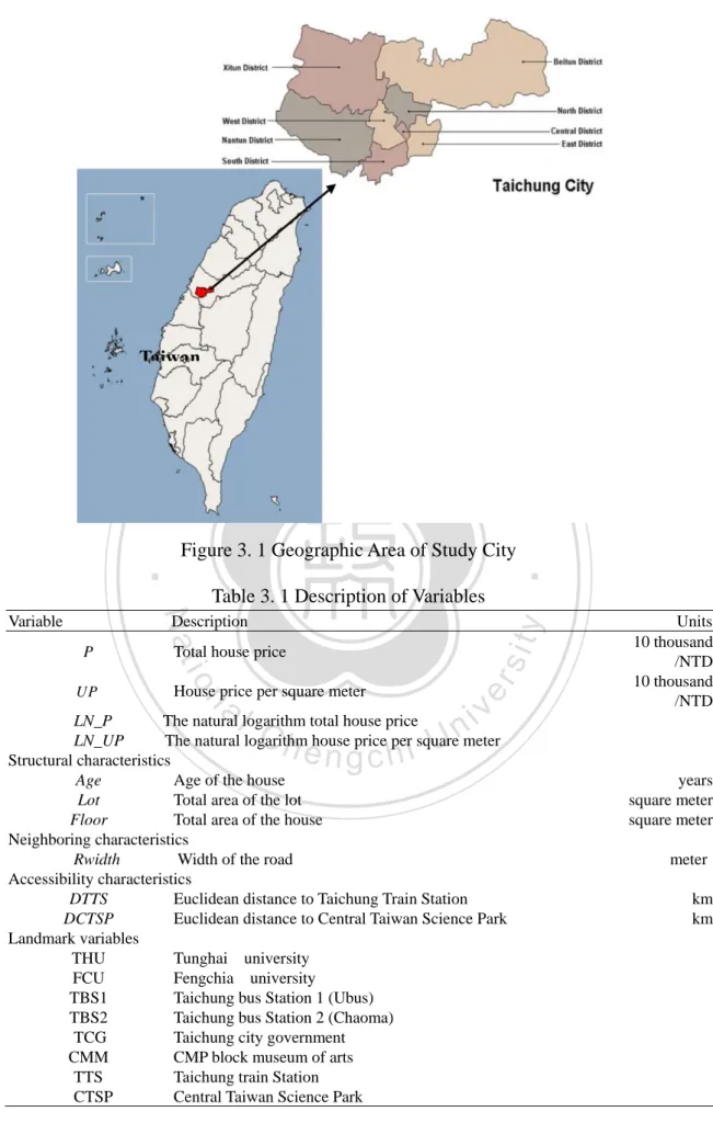
(16) Chapter 3 STUDY AREA DESCRIPTION In recent years, spatial data analysis has received significant awareness and played an important role in social science because of the rapid development of GIS. Although classical statistical methods are attractive in traditional data analysis, they cannot be applied for spatial data. However, spatial statistics methods can give us more specific estimators in structures and processes appearing on real estate market than before. Thus, application of spatial statistics method to real estate analysis seems to be necessary.. 治政 The study area is Taichung city, which is located in 大 the middle part of Taiwan (Fig. 立 3.1). This exhibit shows the city divided into eight districts. The Taichung city center ‧ 國. 學. is in Xitun District. Xitun District is the most popular district in the city. It is located. ‧. in the north-western part of the city. It is also the location of many universities and shopping sites. The Taichung Industrial Park, World Trade Center, and some major. y. Nat. io. sit. transportation stations are also located in the district. Xitun District is the most. n. al. er. popular area with greatest growth in Taichung. Nantun District occupies the. Ch. i n U. v. southwestern-most portions of the city. There is still considerable farmland in this area,. engchi. but since the High Speed Rail 1 (Taichung Station) has started operation in the adjacent Wuri District and there is a growing number of residents. Currently, Nantun is most well known for high property values and expensive, luxurious cottages, which have in turn attracted many large department stores into adjacent areas in Xitun District. Beitun District is the largest district in the city geographically, cover from north to the northeastern of the city. Central District is the smallest and most densely                                                         1. Taiwan High-Speed Rail (HSR) started to serve in early 2007. The total length of Taiwan’s HSR line is 345km. The new rail link is mainly designed to promote balanced regional development. Currently, Taiwan HSR has eight stations, from north to south, Taipei, Banciao, Taoyuan, Hsinchu, Taichung, Chiayi, Tainan and Zuoying (Kaohsiung), respectively. 8 .

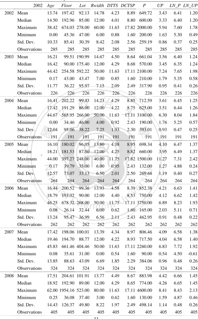
(17) populated district in the city. The Taichung Train Station, Taichung Park, and a large number of traditional businesses are located in this area. This district was used to be regarded as important location of Taichung's major businesses. South District located in the most southern part of the city. East District is on the other side of the tracks from the main part of the downtown area. North District is sited between Central and Beitun Districts, which is one of the well known shopping belt in the city. The national science museum and some department stores are located in this area. West District is famous for the National Taiwan Museum of Fine Arts. A lot of cultural. 政治大 The analytical dataset includes 2,729 duplex residence transactions in Taichung 立. activities are held here.. City from Q1, 2002 to Q4, 2011. The data after 2011 is not available now. The data is. ‧ 國. 學. obtained from Dept of Land Administration, M. O. I. (Official Cadastre Agency) of. ‧. Taiwan. The department provides information for all housing transactions that. sit. y. Nat. occurred during this period and it included the structural characteristics of each. io. er. property such as transaction price, age of house, size of floor and lot, and road width. Through the GIS address matching procedure, all properties are geo-coded; i.e., a. al. n. v i n C his calculated for each latitude and longitude coordinate house. GIS is then used to engchi U calculate Euclidean distances from each house to the Taichung Train Station (TTS). and Central Taiwan Science Park (CTSP) in our empirical analysis. In the estimations, the distances are measured in km and labeled as DTT and DCTSP, respectively. The detail description of the property characteristics is provided in Table 3.1. The descriptive statistics for property characteristics are summarized in Table 3.2. From graphical appearance in Fig. 3.2, the average house price in Taichung city increased almost continuously from 2002 to 2006. After 2007, the house price continued to rise until 2010, and then fell in 2011. 9 .

(18) Taiwan. 立. 政治大. ‧ 國. 學 Table 3. 1 Description of Variables. Nat. Total house price. io. House price per square meter. al. n. UP. sit. P. y. Description. Ch. er. Variable. ‧. Figure 3. 1 Geographic Area of Study City. i n U. v. LN_P The natural logarithm total house price LN_UP The natural logarithm house price per square meter Structural characteristics Age Age of the house Lot Total area of the lot Floor Total area of the house Neighboring characteristics Rwidth Width of the road Accessibility characteristics DTTS Euclidean distance to Taichung Train Station DCTSP Euclidean distance to Central Taiwan Science Park Landmark variables THU Tunghai university FCU Fengchia university TBS1 Taichung bus Station 1 (Ubus) TBS2 Taichung bus Station 2 (Chaoma) TCG Taichung city government CMM CMP block museum of arts TTS Taichung train Station CTSP Central Taiwan Science Park. engchi. 10 . Units 10 thousand /NTD 10 thousand /NTD. years square meter square meter meter km km.

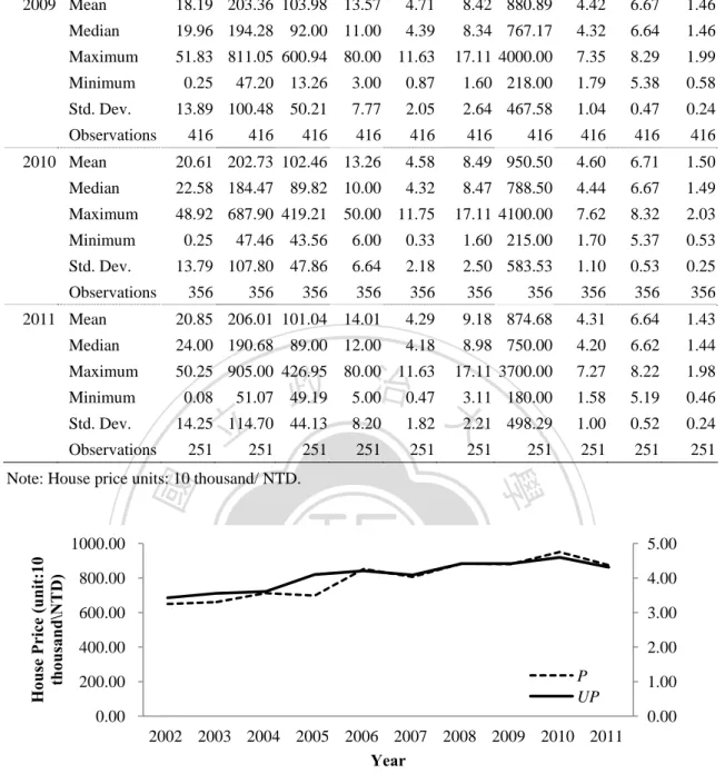
(19) Table 3. 2 Descriptive Statistics of Variables from 2002 to 2011 2002 Age 2002 Mean. Lot. Rwidth DTTS DCTSP. P. UP. LN_P LN_UP. 13.74 197.42 92.13 14.78. 4.23. 8.89 649.72. 3.43. 6.41. 1.20. Median. 14.50 192.96 85.00 12.00. 4.01. 8.80 600.00. 3.33. 6.40. 1.20. Maximum. 38.42 674.03 278.00 60.00 11.63. 17.82 2000.00. 5.94. 7.60. 1.78. Minimum. 0.00. 45.36 47.00. 6.00. 0.88. 1.60 200.00. 1.63. 5.30. 0.49. Std. Dev.. 10.33. 85.41 30.39. 8.42. 2.08. 2.56 259.19. 0.86. 0.37. 0.25. 285. 285. 285. 285. 285. 285. 285. 16.21. 99.51 190.99 14.67. 4.50. 8.64 661.04. 3.56. 6.40. 1.24. Median. 16.42. 90.00 175.40 12.00. 4.29. 8.68 570.00. 3.45. 6.35. 1.24. Maximum. 44.42 254.58 592.22 50.00 11.63. 17.11 2100.00. 7.24. 7.65. 1.98. Observations 2003 Mean. 285. 285. 285. Minimum. 0.17. 43.00 43.47. 7.00. 0.85. 1.60 210.00. 1.79. 5.35. 0.58. Std. Dev.. 11.77. 36.22 95.97. 7.15. 2.09. 2.49 317.90. 0.95. 0.41. 0.26. 226. 226. 226. 226. 226. 226. 3.61. 6.45. 1.25. 3.51. 6.44. 1.26. 6.30. 8.04. 1.84. 1.76. 5.25. 0.57. Observations. 226. 226. 226. 226. Minimum. 4.29 8.85 712.59 治政 17.42 191.29 86.00 12.00 4.22 8.75 625.00 大 44.67 565.95 266.00 50.00 11.63 17.11 3100.00 立 0.00 34.46 46.00 4.00 0.92 2.43 190.00. Std. Dev.. 12.04. 2004 Mean. 16.41 202.22 99.43 14.23. Median. 2.30 393.01. 0.93. 0.47. 0.25. 191. 191. 191. 191. 191. 191. 191. 16.10 180.02 96.05 13.80. 4.38. 8.95 698.34. 4.10. 6.47. 1.37. 18.21 181.53 87.50 12.00. 4.25. 8.82 660.00. 3.95. 6.49. 1.37. Maximum. 17.82 1500.00 11.27. 7.31. 2.42. 191. 191. 44.00 397.27 248.00 40.00 11.75 39.79 35.00. 6.00. 0.95. 2.43 132.00. 1.27. 4.88. 0.24. 73.07 33.13. 6.50. 2.01. 2.50 269.68. 1.19. 0.40. 0.27. 264. 264. 264. 264. 264. 264. 264. 4.21. 6.63. 1.41. 4.12. 6.62. 1.42. 6.89. 8.23. 1.93. Minimum. 4.58 8.39 852.38 a 18.79 193.02 l C 90.00 12.00 4.40 n8.53i v 750.00 46.25 678.32 268.00 11.75 U17.11 3750.00 h e n50.00 i h c g 0.08 26.14 32.44 6.00 0.62 1.60 165.00. 2.03. 5.11. 0.71. Std. Dev.. 13.24. Median Maximum. 16.44 200.52 99.36 13.93. 6.56. 2.11. 2.43 462.95. 0.91. 0.48. 0.22. 262. 262. 262. 262. 262. 262. 262. 17.42 198.06 100.01 13.39. 4.34. 8.97 806.46. 4.09. 6.58. 1.38. Median. 19.46 194.70 88.77 12.00. 4.22. 8.93 717.50. 4.04. 6.58. 1.40. Maximum. 45.83 661.46 404.46 50.00 11.63. 17.11 2260.00. 6.83. 7.72. 1.92. Observations 2007 Mean. 262. 95.47 36.99. sit. 264. er. 264. n. 2006 Mean. 264. io. Observations. y. 0.17. 12.57. Std. Dev.. Nat. Minimum. 191. 95.06 38.22. ‧. Median. 1.93. 學. Observations 2005 Mean. 7.25. ‧ 國. Maximum. 262. 262. Minimum. 0.08. 35.61 31.00. 0.00. 0.54. 1.60. 90.00. 0.54. 4.50. -0.61. Std. Dev.. 13.85. 88.63 43.09. 6.69. 1.85. 2.29 384.06. 0.96. 0.48. 0.26. 324. 324. 324. 324. 324. 324. 324. 17.51 204.61 101.91 13.77. 4.49. 8.67 883.98. 4.42. 6.66. 1.45. Median. 18.92 192.90 89.00 12.00. 4.29. 8.65 774.00. 4.26. 6.65. 1.45. Maximum. 62.00 1954.16 523.00 80.00 11.63. 17.11 4600.00. 8.41. 8.43. 2.13. Observations 2008 Mean. Minimum Std. Dev. Observations . Floor. 324. 0.25. 324. 324. 36.08 37.40. 3.00. 0.62. 1.60 130.00. 1.59. 4.87. 0.46. 14.43 126.37 49.80. 8.22. 1.97. 2.49 498.14. 1.14. 0.48. 0.26. 405 11 . 405. 405. 405. 405. 405. 405. 405. 405. 405.

(20) 2009 Mean. 18.19 203.36 103.98 13.57. 4.71. 8.42 880.89. 4.42. 6.67. 1.46. Median. 19.96 194.28 92.00 11.00. 4.39. 8.34 767.17. 4.32. 6.64. 1.46. Maximum. 51.83 811.05 600.94 80.00 11.63. 17.11 4000.00. 7.35. 8.29. 1.99. Minimum. 0.25. 47.20 13.26. 3.00. 0.87. 1.60 218.00. 1.79. 5.38. 0.58. 13.89 100.48 50.21. 7.77. 2.05. 2.64 467.58. 1.04. 0.47. 0.24. 416. 416. 416. 416. 416. 416. 416. 20.61 202.73 102.46 13.26. 4.58. 8.49 950.50. 4.60. 6.71. 1.50. Median. 22.58 184.47 89.82 10.00. 4.32. 8.47 788.50. 4.44. 6.67. 1.49. Maximum. 48.92 687.90 419.21 50.00 11.75. 17.11 4100.00. 7.62. 8.32. 2.03. Std. Dev. Observations 2010 Mean. 416. 0.25. 416. 47.46 43.56. 6.00. 0.33. 1.60 215.00. 1.70. 5.37. 0.53. 13.79 107.80 47.86. 6.64. 2.18. 2.50 583.53. 1.10. 0.53. 0.25. 356. 356. 356. 356. 356. 356. 356. 20.85 206.01 101.04 14.01. 4.29. 9.18 874.68. 4.31. 6.64. 1.43. Median. 24.00 190.68 89.00 12.00. 4.18. 8.98 750.00. 4.20. 6.62. 1.44. Maximum. 50.25 905.00 426.95 80.00 11.63. 17.11 3700.00 政 5.00治0.47 大3.11 180.00 44.13 8.20 1.82 2.21 498.29. 7.27. 8.22. 1.98. 1.58. 5.19. 0.46. 1.00. 0.52. 0.24. 251. 251. 251. Observations 2011 Mean. Minimum. 356. 356. 0.08. Std. Dev.. 51.07 49.19. 立251 251. 14.25 114.70. Observations. 356. 251. 251. 400.00. ‧ 國. io. 200.00. al. n 0.00. 5.00. 2002 2003. 4.00 3.00 2.00. er. 600.00. Nat. House Price (unit:10 thousand\NTD). 800.00. 251. ‧. 1000.00. 251. 學. Note: House price units: 10 thousand/ NTD.. 251. y. Std. Dev.. sit. Minimum. 416. v i n C h2005 2006 2007 U2008 2009 2004 e n g Year chi. P UP. 1.00 0.00. 2010 2011. Note: The trend of Taichung city house price is shown as UP and P. For UP and P, the trend of the house price is similar (except for 2005). In 2005, average total lot area decreased resulting total house price reduction.. Figure 3. 2 Average House Price for Taichung City by Year. 12 .

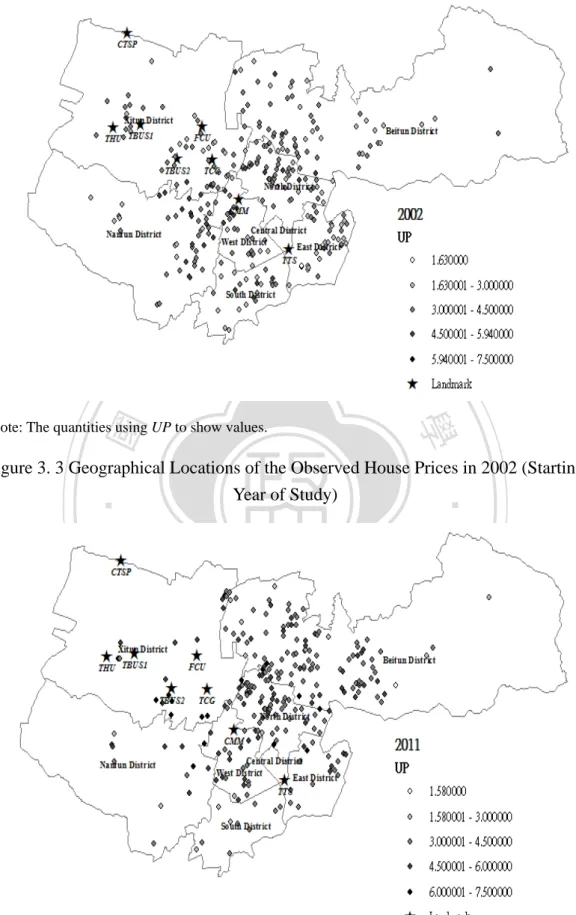
(21) . 學. ‧ 國. 立. 政治大. Note: The quantities using UP to show values.. ‧. Figure 3. 3 Geographical Locations of the Observed House Prices in 2002 (Starting Year of Study). n. er. io. sit. y. Nat. al. Ch. engchi. i n U. v. Note: The quantities using UP to show values.. . Figure 3. 4 Geographical Locations of the Observed House Prices in 2011 (Ending Year of Study) 13 .

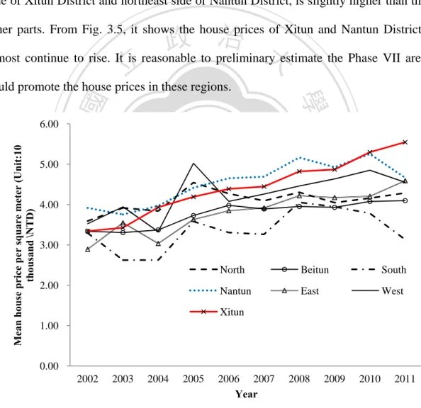
(22) Fig. 3.3 and 3.4 show the geographical locations of observed house prices in 2002 and 2011, respectively. From the initiatory information, the western part of the area has experienced relatively higher in house price. It should be noted that the HuiLai Urban Land Consolidation Area (Phase VII), which is located at the new city center in Taichung city, crowded with the new city hall, residential buildings, and department stores. It is speculated that the Phase VII would drive the surrounding house prices. As shown in Fig. 3.3 and 3.4, the house price in Phase VII area, which contains south side of Xitun District and northeast side of Nantun District, is slightly higher than the. 政治大 almost continue to rise. It is reasonable to preliminary estimate the Phase VII area 立 other parts. From Fig. 3.5, it shows the house prices of Xitun and Nantun Districts. could promote the house prices in these regions.. ‧ 國. y. sit. n. al. er. io. Mean house price per square meter (Unit:10 thousand \NTD). Nat. 4.00. ‧. 5.00. 學. 6.00. 3.00. Ch. 2.00. e n g cNorth hi. i n U. Nantun. v. Beitun. South. East. West. Xitun 1.00. 0.00 2002. 2003. 2004. 2005. 2006 2007 Year. 2008. 2009. 2010. 2011. Note: UP is used to illustrate the trend of different district house price. In central districts, there are no residential transactions in some years.. Figure 3. 5 Yearly Average House Price for Each District in the Study Area. 14 .

(23) Chapter 4 GEOGRAPHICALLY WEIGHTED REGRESSION APPROACH Using global model to the empirical analyses of spatial data is the conventional approach. The expression ‘global’ means that all the spatial data are used to estimate an equation that is an average of the circumstances that occur throughout the study area in which the data have been measured (Matthews and Yang, 2012). The primary assumption in a global model is that the relationships between the dependent variable. 政治大. and explanatory variables are stationary across space. However, in some cases, the. 立. relationships between variables might be non-stationary and variable spatially. ‧ 國. 學. (Brunsdon et al., 1996; Lloyd, 2011). Spatial non-stationary exists when the equal incentive triggers a different reaction in different locations of the study area. If. ‧. non-stationary exists within the study area, then there is a proposition, special. Nat. sit. y. procedures, to deal with the phenomenon. The geographically weighted regression is. n. a. l C Model) 4.1 Linear Regression (Global. hengchi. er. io. introduced for investigating this problem.. i n U. v. The linear regression is a general technique for investigating the linkage between dependent variable and explanatory variables, and has been widely used in real estate assessment. However, in some previous studies, the technique ignores location in its analysis of relationships between variables. The elements of a regression model, X and y , are a matrix including a set of independent variables and. a vector of. dependent variables, respectively. The relationship between these is written as:. yi   0   X ir  r   i. (4.1). r 1.   N (0,  2 I ) where  is a vector of regression coefficients and  is a vector of error terms. This 15 .

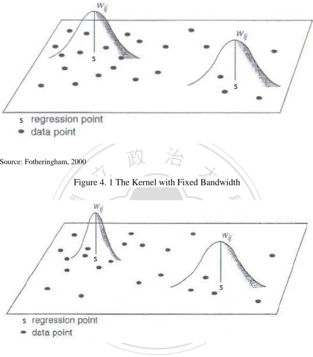
(24) would produce (Ordinary Least Squares method, OLS) estimation for the parameter.  r in the model equal to: ˆ  ( X T X ) 1 X T y. (4.2). In this way, it doesn’t consider the geographical data with each observation corresponds to a geographical location. This implies spatial characteristic doesn’t play a role in this model. However, there may be phenomena when the character of such models is not fixed over space. Several precise techniques of incorporating space have been explored. This situation is considered as spatial non-stationary (Brunsdon et al.,. 政治大 In next section, the Geographically Weighted Regression is used for a particular 立. 1998).. technique of detecting whether there is spatial variability. Besides this methodology,. ‧ 國. 學. one example of the technique will be given.. ‧. 4.2 Geographically Weighted Regression (Local Model). Nat. sit. y. In geography and other related science, Geographically Weighted Regression (GWR). n. al. er. io. is one of spatial regression techniques. Applying GWR to real estate analysis allows. i n U. v. further spatial distribution of prices by including spatial heterogeneity of phenomenon.. Ch. engchi. When GWR is applied, key decisions concerns the choice of weighting function (the shape of the kernel) and the bandwidth of the kernel (Lloyd, 2011). Based on kernel analysis, the kernel function is distributed across the study area and the kernel weights observations within its sphere of function. The kernel function can be used as the weight allocated to observations is a function of distance from the centre of the kernel. A kernel function is showed in Fig. 4.1 (fixed bandwidth)2and Fig 4.2 (adaptive.                                                         2. The spatial context (the Gaussian kernel) used to solve each local regression analysis is a fixed distance. 16 .

(25) bandwidth)3.. Source: Fotheringham, 2000. 立. 政治大. Figure 4. 1 The Kernel with Fixed Bandwidth. ‧. ‧ 國. 學. n. er. io. sit. y. Nat. al. Ch. engchi. i n U. v. Source: Fotheringham, 2000. Figure 4. 2 The Kernel with Adaptive Bandwidth Through incorporating the dependence and explanatory variables of features within the bandwidth of each target feature, GWR can create these separate equations.                                                         3. The spatial context is a function of a specified number of neighbors. Where feature distribution is. dense, the spatial context is smaller; where feature distribution is sparse, the spatial context is larger.. 17 .

(26) Particularly, the result of GWR is local models matching a particular location rather than one global model for the whole market. It means every single location obtains its own regression parameters (Kulczycki and Ligas, 2007). GWR model can be written as follows: y ( si )   0 ( si )    r ( si )  xir   ( si ) ,. i  1,..., n. (4.3). r 1. where si is the location of i-th observation point,  r ( si ) is the r -th regression parameter in point i-th ,  (si ) is error term, and xir is the r -th characteristic of. 政治大 depending on locations to estimate local parameters  ( s ) of GWR model. 立. i-th observation point. Using weighted least squares method with weighting matrix r. i. ‧ 國. 學. For such defined model, the parameters for GWR may be estimated by solving:. ˆ ( si )  ( ΧT W( si ) Χ)1  ΧT W( si )y. (4.4). ‧. where weighting matrix W( si ) is an n by n matrix, the diagonal elements of. sit. y. Nat. io.  wi1 0 0 w i2 W( si )      0 0. n. al. Ch.  0   0      win . engchi. er. which are the geographical weightings of observations around point i :. i n U. v. (4.5). From the assumption, locations closer to i have greater weight than these ones further away. Several weighting function have been used. A widely used weighting scheme is Gaussian function. With this function, a weight at observation i is obtained with: wij  exp  0.5( d ij /  ) 2 . (4.6). where d ij is the Euclidean distance between the location of i and j ;  is the bandwidth of the kernel. Alternative weighting function could be 18 .

(27)  1  (d /  )2  2 if d   ij ij  wij    otherwise 0. (4.7). Based on Brunsdon et al. (1998), this function will be referred to as kernel function (denoted as  ( d ij ) ). In each situation, the constant  supplies some control of the range of influence of the geographical observation point. However, the value of weight would decay gradually with distance rather than suddenly falling to zero when a certain distance is reached. Generally, desirable features of a kernel function  are.  (0)  1,  lim d   ( d )  0  is a monotone decreasing function for positive numders. . 政治大. 立. (4.8). 學. ‧ 國. For each location si , the fitted values of y is obtained from the formula:. ‧. yˆ ( si )  xi  β( si ). Nat. y. (4.9). er. io. sit. And a set of residuals at all locations si :. al. n. v i n  (s C y ( s )  yˆ ( s )  y ( s )U ) h e n g c h i  x  β( s ) i. i. i. i. i. i. (4.10). Through appropriate statistical test, a basis of determined parameters and other quantities to describe the model is constructed. The detail procedure test is mentioned in Brunsdon et al. (1998). GWR is deliberated to detect the problem, “Do relationships vary across space?” It is important to note that GWR approach does not assume that relationships vary across space but is a means to identify whether or not they do (Matthews and Yang, 2012). GWR can be applied as a diagnostic tool to recognize the phenomenon of spatial variation. If the relationships do not vary across space, the global (OLS) model 19 .

(28) is an appropriate measurement for the data. Furthermore, the Akaike Information Criterion (AIC) index is used to compare the fitted results from the global (OLS) model with those from the local (GWR) model. The AIC index would disclose whether the spatial viewpoint will significantly improve the model fitted effect.. 4.3 Empirical Analysis In this section, a practical example of GWR will be given. The GeoDa software and GIS software package (ArcGIS) are integrated for model parameter estimation and mapping. This will be based on data taken from Dept of Land Administration, M. O. I.. 政治大. (Official Cadastre Agency) of Taiwan. The analytical dataset consists of 251 duplex. 立. residence transactions in Taichung city during 2011. The geographic area of this study. ‧ 國. 學. is shown in Fig.3.1 (Chapter 3). The Dept of Land Administration provides information for all housing transactions that occurred during this period and it. ‧. included the structural characteristics of each property such as transaction price, age. Nat. sit. y. of house and size of lot and floor, and road width. The detail description of the. n. al. er. io. property characteristics is provided in Table 3.1.. i n U. v. In this case, LN_P is the natural logarithm total transaction price of the house. Ch. engchi. which is used as the dependent variable in the hedonic regression estimations. “Age” means the age of house which is one of the negative effects affecting house price. Thus it is expected to have a negative coefficient for Age. Lot and Floor are the total areas of the lot and house, respectively, which measured in square meter. The size of Lot and Floor are expected to positively affect the Price. Rwidth is the width of the road, and it is expected to contribute to a higher house value since this would indicate more convenient of communication. DTTS and DCTSP represent the distance to Taichung Train Station (TTS) and Central Taiwan Science Park (CTSP), respectively, and estimate the effect of nearby amenities on house prices. However, the nearby 20 .

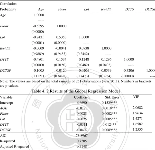
(29) amenities may increase or decrease housing prices. Hence the direction of price effects is not assumed. 4.3.1. Results of Global (OLS) Model. Firstly, in order to understand how the independent variables impact on price, the multicollinearity is worthy of further investigation. Therefore, the multicollinearity between these independent variables in this model is tested with the correlations matrix in Table 4.1. As the results, all absolute values of the correlation coefficient are almost less than 0.5. The largest correlation is between Floor and Lot and this is quite. 政治大 might be a phenomenon of luxury as compared to the past. Then the multicollinearity 立. intuitive. The maximum negative correlation is between Floor and Age, and this. diagnostics are conducted by VIF (Variance Inflation Factor) of the predictor variables. ‧ 國. 學. for further determination. In general, VIF values above 10 suggest a mulitcollinearity. sit. y. Nat. had no significant problems with collinearity.. ‧. problem. Table 4.2 shows the VIF value for each variable and indicates that the data. io. er. Second, the OLS regression model will be measured. Based on the principle of best fit, Rwidth is less statistically significant, and then it is excluded from the initial. al. n. v i n model. From the results shown C in Table be seen that, at global OLS model, h e n4.2,gitccan hi U. every variable has a statistically significant coefficient. About 73.8967% of the variations in house prices are explained by the variations in the selected explanatory variables indicated by the R-squared statistic. As expected, Age decreases the house price by about 0.0123%. Both Lot and Floor positively affect the house price. Then, the accessibility variables (DTTS and DCTSP) are statistically significant for distances to Taichung Train Station and Central Taiwan Science Park, respectively. The coefficients for DTTS and DCTSP are both negative.. 21 .

(30) Table 4. 1 Correlation Matrix of Variables used in Estimations Correlation Probability Age. Age. Floor. Lot. Rwidth. DTTS. DCTSP. 1.0000 -----. Floor Lot Rwidth DTTS DCTSP. -0.5395. 1.0000. (0.0000). -----. -0.2431. 0.5353. (0.0001). (0.0000). -----. -0.0009. -0.0041. 0.0738. 1.0000. (0.9889). (0.9483). (0.2442). -----. -0.4801. 0.1534. 0.1248. 0.1296. 1.0000. (0.0000). (0.0150). (0.0482). (0.0402). -----. -0.1005. 0.0120. 0.0204. -0.0539. -0.3206. 1.0000. 1.0000. (0.1121) (0.8498) (0.7473) (0.3954) (0.0000) ----Note: The values are based on the total samples of 251 observations (year 2011). Numbers in brackets are p-values.. 0.1529*** 0.0018*** 0.0002*** 0.0005*** 0.0124** 0.0089***. y. ‧. ‧ 國. 學. 6.6690 -0.0123 0.0023 0.0025 -0.0311 -0.0409. Nat. Variable Intercept AGE Floor Lot DTTS DCTSP. 政治大 Table 4. 2立 Results of the Global Regression Model Coefficient Std. Error. VIF 2.0682 1.9634 1.4271 1.6582 1.2555. sit. n. al. er. io. AIC 73.8967 R-squared 0.7205 Adjusted R-squared 0.7148 Note: Number of included observations=251. The dependent variable is the natural logarithm total house price (LN_P). Large Variance Inflation Factor, VIF (> 7.5, for example) indicates explanatory variable redundancy. ** Denotes 5% statistical significance; *** Denotes 1% statistical significance. Ch. engchi. i n U. v. 4.3.2. Results of Local (GWR) Model. In this section, the results of using a GWR model for the house price data are discussed. Firstly, 4-indicator summary of parameter estimation describes the degree of variability in the parameter estimation (the 4-indicator summary is based on the maximum, minimum, median, and mean local parameter estimates reported in the GWR model). Next, in order to know the heterogeneity in individual parameters, GWR technique can visualize the local parameter estimates. Each parameter can be mapped as surface illustration of the spatial variation (Matthews and Yang, 2012). In 22 .

(31) GWR, the regression is re-centered many times (on each observation) to generate locally GWR parameter results. These local GWR results generate a complete map of the spatial variation of the parameter estimates. The local statistics can take on different values at each location. GWR results is unlike global model results, it is mappable and given a very large number of potential parameters estimation. It is almost essential to map the potential parameters in order to make some sense of the patterns they display (Matthews and Yang, 2012). There is a short summary of results obtained from application GWR to house price. 政治大 entire study area, and they change along with location. Furthermore, AIC index also 立. assessment (Table 4.3). The regression parameters seem not to be constant over the. shows slight decline (from 73.8967 to 67.5369). The R-squared (Adjusted R-squared). ‧ 國. 學. value increases when GWR tool are considered in the model. Comparing the GWR. ‧. diagnostics to the OLS diagnostics, the GWR performs better model fitting.. Lot DTTS DCTSP AIC R-squared. (39.0464). (39.4201). -0.0126. -0.0131. Ch. y. n. Floor. al. 6.8192. sit. io. AGE. 6.7975. GWR MEAN. 6.7691. 6.6757. (38.2937). (39.0262). -0.0122. -0.0120. er. Intercept. Nat. Table 4. 3 Results of the Local Regression Model GWR MAX GWR MIN GWR MEDIAN. v ni. (-6.9180). (-7.1202). (-6.6844). (-6.5163). 0.0023. 0.0022. 0.0023. 0.0023. (10.7481). (10.2338). (10.8866). (10.7041). 0.0026. 0.0026. 0.0026. 0.0028. (5.4094). (5.3724). (5.4700). (5.7121). -0.0386. -0.0447. -0.0348. -0.0364. (-2.6948). (-3.1202). (-2.3916). (-2.5382). -0.0511. -0.0492. -0.0508. -0.0424. (-4.9624). (-4.8380). (-4.8423). (-4.1761). engchi U. 67.5369 0.7347. Adjusted R-squared 0.7255 Note: In this case, adaptive kernel type (Gaussian kernel) is used. The spatial context is a function of a specified number of neighbors. Where feature distribution is dense, the spatial context is smaller; where feature distribution is sparse, the spatial context is larger. The dependent variable is the natural logarithm total house price (LN_P). Numbers in brackets are t-values.. 23 .

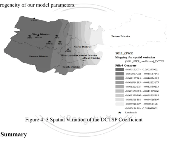
(32) Next, to give a brief display of the spatial variation, Fig.4.3 is taken into consideration. This is interesting when the coefficient takes both high and low values. In particular, in Nantun district and Xitun district, there are strong negative relationship (the house prices decrease as the distance to the CTSP increases) whereas in other areas the relationship is reduced gradually. After statistical detection and schema description, the direct evidence indicates that the characteristic influence isn’t the same in all regions. Thus, GWR model can help to analyze the spatial heterogeneity of our model parameters.. 立. 政治大. ‧. ‧ 國. 學. n. er. io. sit. y. Nat. al. Ch. engchi. i n U. v. Figure 4. 3 Spatial Variation of the DCTSP Coefficient. 4.4 Summary In this chapter, the technique for producing visual local regression coefficients is discussed. In the past, the coefficients for a global regression may fail to notice geographical features in the relationships between variables. However, the GWR technique has provided a straight and reasonable approach to deal with the problem. GWR is a helpful tool for investigation that produces a set of location-specific parameter estimates which can be analyzed and mapped to offer information on spatial non-stationary in regression parameters. 24 .

(33) Chapter 5 MEASUREMENTS OF SPATIAL AUTOCORRELATION AND SPATIAL MODELS Generally, classical statistical theory assumes that observations are independent and identically distributed ( i.i.d.), usually following a normal distribution. The covariance term is set to zero in this assumption that simplifies the mathematical statistical theory. However, correlated sample violated the first i.i.d. assumption. On the basis of this opinion, statisticians began to search situations in which the independence assumption.. 政治大. Recently, attention is paid to spatial statistics in real estate research.. 立. Spatial statistics contains spatial autoregression and geostatistics. These two. ‧ 國. 學. branches are developed separately over a number of decades. In a very general sense, spatial statistics is concerned with the statistical analysis of geo-referenced data.. ‧. These observations are correlated strictly owing to their relative locations. In other. y. Nat. io. sit. words, spatial autocorrelation means data located relatively close together. n. al. er. geographically and tend to be correlated. In this chapter, the spatial autocorrelation is. Ch. i n U. v. addressed and spatial econometrics (autoregressive) models are illustrated.. 5.1 Spatial Autocorrelation. engchi. Moran’s I statistic (Moran, 1948) is the most widely used index of spatial. After more than half century, it is still typical in examination of spatial autocorrelation. The Moran’s I statistic for spatial autocorrelation is given as:. 25 .

(34) n. I. n. n. i 1 j 1. i 1 j 1. n.  ( y  y) n. n. 2. /n.  ( y  y) i 1. n. i 1 j 1. n. ij. 2. i.  w ( y  y )( y. n. (5.1). n. i. i 1. . n.  wij ( yi  y )( y j  y ) /  wij. i. j. /n.  y). n.  wij.  ( y  y). i 1 j 1. i 1. 2. i. Where wij is a binary (i.e., 0 or 1) indicator variable signifying whether location i and j are nearby or not. It means an element of a matrix of spatial weights. Then, n is equal to the total number of features.. 政治大. The zI  score for the statistic is computed as:. zI . 學. I  EI  VI . (5.2). ‧. io. y. V  I   E  I 2   E  I . 2. al. sit. Nat. E  I   1/(n  1). er. where:. ‧ 國. 立. (5.3). n. v i n C h are either bothUlarger than the mean or both When values for adjacent attributes engchi smaller than the mean, the cross-product will be positive. On the contrary, one value is less than the mean and the other is larger than the mean, the cross-product will be negative. If the values are cluster spatially, the Moran's Index will be positive (high values cluster near other high values; low values cluster near other low values). If the high values tend to near low values, the Moran's Index will be negative. When positive cross-product values are equal to the amplitude of negative cross-product values, the Moran's Index will be near zero. In general, the Moran's Index is bounded by -1 and +1. After the Index value is obtained from spatial autocorrelation tool, the 26 .

(35) expectation and variance of the Index value are calculated. Then, the zI  score and p  value indicate whether this spatial autocorrelation is statistically significant or not. (Mitchell, 2005).. 5.2 Spatial Lag Model (SLM or SAR) This section illustrates the estimation by means of maximum likelihood of spatial hedonic price model (or spatial autoregressive model) that contains a spatially lagged dependent variable. Unlike the traditional approach, which uses eigenvalues of the weighting matrix, this method is well suited to the estimation in situations with very large data sets.. 立. 政治大. 學. y  Wy  X   .   N (0,  2 I ). (5.4). ‧. ‧ 國. Formally, spatial lag model is expressed as (Anselin, 2003):. Nat. sit. y. where y is a vector of dependent variable, W is spatial weights matrix, and  is a. n. al. er. io. coefficient on the spatially lagged dependent variable, Wy . Then, X is a matrix of. v. explanatory variables,  is estimated parameter, and  is a vector of error terms (i.i.d.).. Ch. engchi. i n U. 5.3 Spatial Error Model (SEM) Next, this part shows the estimation by means of maximum likelihood of spatial hedonic price model (or spatial autoregressive model) that contains a spatial autoregressive error term. Formally, spatial error model is expressed as (Anselin, 2003):. y  X    W   u. (5.5). u  N (0,  I ) 2. 27 .

(36) where y is a vector of dependent variable, X is a matrix of the explanatory variables, W is the spatial weight matrix, and  is a coefficient on the spatially correlated errors. Then,  is a vector of spatially autocorrelated error terms, u is a vector of error terms (i.i.d.), and  is estimated parameters.. 5.4 Empirical Analysis The case study is concerned with the analysis of the spatial autocorrelation using the data described in chapter 3. The GeoDa software and GIS software package (ArcGIS) are integrated for model parameter estimation and mapping. The hedonic price model. 政治大. is considered over the study area. However, hedonic price parameters (OLS model). 立. are usually estimated using procedures that assume independent observations. If. ‧ 國. 學. hedonic residuals are spatially autocorrelated, the resulting parameter estimation will be inefficient and will be biased (Basu and Thibodeau, 1998). The treatment which. ‧. considers and expresses such a correlation in set of market information is spatial. Nat. sit. n. al. er. io. spatial issues.. y. hedonic price models which are generalizations of OLS model with reference to. i n U. v. In our empirical analysis, with the SLM and SEM model, the parameter of a. Ch. engchi. hedonic price model may be made functions of other attributes including Age, Floor, Lot, DTTS and DCTSP in parameter estimation. LN_P is used as the dependent variable in the hedonic regression. For example, the analytical dataset consists of 251 duplex residence transactions in Taichung city during 2011. In addition, in order to identify which model is suitable, some tests are used on model specification to identify by Lagrange multiplier test: LM (lag) , Robust LM (lag) , LM (error) and Robust LM (error) .. According to spatial autocorrelation coefficient (Moran’s I) that is a measurement 28 .

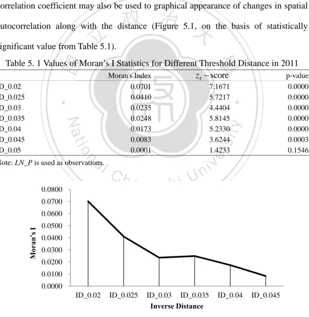
(37) of cluster, the values of distinguished characteristic are determined by other surrounded values of the characteristics. On the basis of Moran’s I statistics, the significance tests of spatial autocorrelation may be created for the null hypothesis H 0 is no significant spatial autocorrelation and alternative hypothesis H 1 is spatial autocorrelation occurrence. Table 5.1 presents values of Moran’s I statistics based on spatial weight matrix constructed on the basis of inverse distance based on criterion and the significance level of the statistics, for different distance thresholds. Moran’s I correlation coefficient may also be used to graphical appearance of changes in spatial. 政治大. autocorrelation along with the distance (Figure 5.1, on the basis of statistically. 立. significant value from Table 5.1).. ‧ 國. 學. Table 5. 1 Values of Moran’s I Statistics for Different Threshold Distance in 2011 zI  score Moran's Index p-value. n. 0.0800. Ch. engchi. 0.0000 0.0000 0.0000 0.0000 0.0000 0.0003 0.1546. y. sit. er. io. al. Note: LN_P is used as observations.. 7.1671 5.7217 4.4404 5.8145 5.2330 3.6244 1.4233. ‧. 0.0701 0.0410 0.0235 0.0248 0.0173 0.0083 0.0001. Nat. ID_0.02 ID_0.025 ID_0.03 ID_0.035 ID_0.04 ID_0.045 ID_0.05. i n U. v. 0.0700. Moran's I. 0.0600 0.0500 0.0400 0.0300 0.0200 0.0100 0.0000 ID_0.02. ID_0.025. ID_0.03 ID_0.035 Inverse Distance. ID_0.04. ID_0.045. Note: Graphical appearances are based on Moran’s I ( z I  score ) that are statistically significant at least 1% level (Table 5.1).. Figure 5. 1 Changes in Spatial Autocorrelation Along with the Distance 29 .

(38) The Spatial Autocorrelation (Moran’s I) tool returns five values: the Moran's Index, Expected Index, Variance, zI  score , and p-value. The results of graphical summary are shown as a figure (Fig.5.2).. 立. 政治大. ‧. ‧ 國. 學. n. er. io. sit. y. Nat. al. i n U. v. Figure 5. 2 Graphical Summary of Spatial Autocorrelation Reports in 2011 (ID_0.04). Ch. engchi. Table 5.2 shows the results from the estimation conventional OLS, SLM and SEM models. The OLS regression diagnostics reveal considerable and heteroskedasticity (Koenker-Bassett statistic)4 and spatial autocorrelation (Moran’s I¸ Table 5.1). By comparing the values for SLM to those for OLS, an increase in the Log-Likelihood is noticed from -30.9484 to -29.1570. The improved fitting for the added variable (the spatially lagged dependent variable), the AIC (from 73.8967 to 72.3139) decreases relative to OLS, suggesting an improvement for the spatial lag                                                         4. The Koenker-Bassett statistic (Koenker's studentized Bruesch-Pagan statistic) is a test to determine whether the explanatory variables in the model have a consistent relationship to the dependent variable both in geographic space and in data space. 30 .

(39) specification. There are some minor differences in the significance of the other regression coefficients between the SLM model and the OLS model: more importantly, the significance of DTTS changes from p < 0.05 to p < 0.01. The magnitude of all the estimated coefficients is also affected. To some extent, the explanatory power of these variables that is attributed to their neighboring locations. This is picked up by the coefficient of the spatially lagged dependent variable. By comparing the values of SEM to those for OLS, an increase in the Log-Likelihood is noticed from -30.9484 (for OLS) to -27.1359. The improved fit for. 政治大 66.2718) decreases relative to OLS, suggesting an improvement of fit for the spatial 立. the added variable (the spatially correlated error variable), the AIC (from 73.8967 to. error specification.. ‧ 國. 學. Next is the comparison between Spatial Error and Spatial Lag Models. Following. ‧. the comparison steps, both LM (lag) and LM (error) are significant, but of the robust. Nat. io. sit. y. forms, the Robust LM (error) statistic is highly significant (p < 0.01), while the Robust. er. LM (lag) statistic is not (p>0.1). In 2011, the SEM appeared to be more appropriate. al. n. v i n model (residuals from the OLSC model highly correlated), h e n g c h i U and it gets better fit to the empirical data measured by Log Likelihood and AIC.. From Moran Scatter Plot (Fig. 5.3 to Fig. 5.5), the Moran’s I are 0.0422, 0.0098 and -0.0037, respectively. This indicates that including the spatially autoregressive error term in the model has eliminated mostly spatial autocorrelation. In other annual results, all of spatial models show better fit. There are some minor differences in the significance of the other regression coefficients. Such as in 2006, DTTS changes from p < 0.05 (OLS) to p > 0.1(SEM); DCTSP changes from p < 0.01(OLS) to p < 0.1(SEM). Comparison between SLM and SEM, except for 2002, 2005 and 2011, the SLM provides better fit. The annual results from the estimation 31 .

(40) OLS, SLM and SEM models are shown in appendix3. The SLM and SEM models are closely related to each other mathematically, but their economic interpretations are slightly different. The relevance of one model versus another depends on the particular application at hand. For example, a SEM is preferred over a SLM if the spatial pattern of residuals is considered as potentially valuable information (Yoo and Kyriakidis, 2009). The SLM differs from the spatial SEM. The spatial SEM is based on the assumption that there are omitted variables in the hedonic price equation and the spatial dependence of the error term is due to those. 政治大. spatially varying omitted variable(s) (Anselin, 1998).. 立. DTTS. R-squared Log Likelihood. 0.0022. 0.0002***. -0.0125. 0.0017***. 0.0023. 0.0002***. 0.0023. 0.0002***. 0.0025. 0.0005***. 0.0026. 0.0005***. 0.0029. 0.0005***. -0.0311. 0.0124**. -0.0411. 0.0137***. -0.0340. 0.0147**. 0.0089***. -0.0381. 0.0088***. -0.0353. 0.0119***. 0.6438. 0.2160***. -0.0409. al. 0.7205 -30.9484. VALUE. LM (error). 0.0017***. 0.0018***. TEST. Robust LM (lag). -0.0133. -0.0123. 73.8967. LM (lag). 0.1853***. 1.6764***. AIC Koenker-Bassett. 6.6648. 4.4845. n. . 0.2537. Std. Error. 0.1529***. io. DCTSP. 0.3325. Coefficient. Ch. 0.7248. e n g-29.1570 chi 72.3139. y. Lot. Std. Error. 6.6690. Nat. Floor. Coefficient. sit. Age. Std .Error. SEM. ‧. Intercept. Coefficient. SLM. er. . OLS. 學. Variable. ‧ 國. Table 5. 2 The Results form Estimation OLS, SLM and SEM Models in 2011. i n U. v. 0.7303 -27.1359 66.2718. 46.4380*** 9.5198*** 0.0002 21.8941***. 12.3744*** Robust LM (error) Note: Number of included observations=251. The dependent variable is the natural logarithm total house price (LN_P). Spatial weight matrix with threshold distance is 0.04 m. * Denotes 10% statistical significance; ** Denotes 5% statistical significance; *** Denotes 1% statistical significance. 32 .

(41) 政治大 Figure 5. 3Moran Scatter Plot for OLS_Residue 立 ‧. ‧ 國. 學. n. er. io. sit. y. Nat. al. Ch. engchi. i n U. v. Figure 5. 4Moran Scatter Plot for Lag_Residue. 33 .

(42) 政治大 Figure 5. 5Moran Scatter Plot for Error_Residue 立. ‧ 國. 學. 5.5 Summary. In this chapter, two real estate questions are explored (i) whether our analysis data are. ‧. spatial autocorrelation and (ii) whether spatial hedonic price models increase. Nat. sit. y. traditional hedonic (OLS) price model prediction precision. After empirical analysis,. n. al. er. io. the datasets are found to be spatially autocorrelated. Compared to OLS model, spatial. i n U. v. hedonic price models (SLM and SEM) get better fit to the empirical data.. Ch. engchi. Results from classical regression are only reliable when the model and data meet the assumption (i.i.d.). If spatial autocorrelation is statistically significant, it means the model is not specific. This may be missing an important explanatory variable. If the key missing variables can’t be identified, regression results are inefficient. However, the spatial autoregression approach can be used to deal with spatial autocorrelation problems and offers improved predictions.. 34 .

(43) Chapter 6 GEOSTATISTICAL APPROACH The efficacious modeling of housing prices through the use of numerical methods relies on knowledge of the spatial variation of the observed variables. Estimation of housing prices on a regular mesh of grid points, from its measurement at random points, containing the area of interest is necessary to implement various house price simulation models for sustainable monitoring of housing price volatility. Geostatistics relies on both statistical and mathematical methods, which can be. 政治大. used to create surfaces and assess the uncertainty of predictions (Johnston et al., 2003).. 立. These techniques have the ability of producing a prediction surface and they can also. ‧ 國. 學. provide some measurement of the accuracy of the predictions. Geostatistics originated from the mining industry with the estimation of gold mines and the African engineer. ‧. D.G. Krige gave his name to the famous methods of kriging. This domain was then. Nat. sit. y. developed by G. Matheron in 1963.. n. al. er. io. In recent years, geostatistics is used in real estate (Tsutsumi and Seya, 2008;. i n U. v. Chica-Olmo, 2007; Bourassa et al., 2007; Dubin, 1998; Basu and Thibodeau, 1998).. Ch. engchi. The geostatistical technique of kriging allows for the estimation of the interested variable at a specific location based on data about the variable itself. This ability is an important advantage when the sample size for the interested variable is small or shortage. As this information of housing prices is available at limited and irregularly spaced points, estimation of house prices at the regular grid points is necessary to understand the spatial and temporal behavior of house price in study area. Kriging can obtain the most accurate estimation and enables the quantification of corresponding estimation errors, thus it is more suitable for the above purpose. House prices are spatially autocorrelated because properties in close proximity tend 35 .

(44) to have similar structural characteristics. This is a natural effect of the actuality that spatially adjacent properties tend to be developed at about the same time. Besides, properties within the same area share main region amenities. House price are likely to be spatially autocorrelated in neighborhoods where dwellers follow alike patterns. Spatial autocorrelation in house prices has assumed that the correlation structure is isotropic in most studies. The correlation of pairs of observations is only a function of the distance between properties while the direction separating the properties is ignored. However, some studies have found that the intensity of spatial correlation. 政治大 et al., 2011). Hence, this assumption is reckless if spatial dependence changes with 立 often decreases differently in different directions (such as Gillen et al., 2001 and Zhu. the distance and the direction separating points in space.. 學. ‧ 國. direction. Spatial data is anisotropic when spatial autocorrelation is a function of both. ‧. In this chapter, it is attempt to measure the effect of location on residential house. sit. y. Nat. prices and endeavor to integrate spatial and a spatial data in terms of developing a. io. er. dynamical exploration. Firstly, the spatial variation of the observations using the semi-variogram is quantified and fitted with the experimental semi-variograms in. al. n. v i n C h parametric model. (spherical) Then, engchi U. different directions by. utilizing the fitted. semi-variogram function, ordinary kriging on the house prices based on the model and produced a set of contour maps is performed for further investigation. Finally, the prediction of local housing price is made by a multivariate spatial method: cokriging.. 6.1. Semi-Variogram The semi-variogram  ( h ) is necessary to solve the ordinary kriging system and defined as the expected squared increment of the values between a pair of locations at distance h . It summarizes the relationship between differences in pairs of measurements and the distance of the corresponding points from each other. The 36 .

(45) empirical semi-variogram examines how the spatial autocorrelation between observations. Let y(si ) denotes the house price of observed sit si . For a stationary5 process y(si ) , the variogram is defined or named as semi-variogram. The method of estimation for an empirical semi-variogram (Matheron, 1963) is.  y (h) . NP ( h ) 1 2  y ( si  h)  y ( si )   2 NP ( h ) i 1. (6.1). where y ( si ), y ( si  h) are the house prices at locations si and si  h , respectively. It. 立. means that each variable y(si ). 政治大 takes different value and correlates to its spatial. ‧ 國. 學. location. NP( h) means the number of h distant pairs.. Furthermore, experimental calculation can reveal a very different behavior of the. ‧. experimental semi-variogram in different directions. This is called an anisotropic. sit. y. Nat. behavior. Spatial data is anisotropic when spatial autocorrelation is a function of both. n. al. er. io. the distance and the direction separating points in space. As semi-variogram models. i n U. v. are defined for the isotropic case, it is needed to examine transformations of the. Ch. engchi. coordinates which allow obtaining anisotropic random functions from the isotropic models. In practice, anisotropies are detected by inspecting experimental semi-variograms in different directions and are included into the model by rotating predefined anisotropy parameter (Wackernagel, 1995). Anisotropic semi-variograms have been examined such as Gillen et al., 2001 and Zhu et al., 2011, provided an exact test for anisotropic spatial autocorrelation. In order to calculate the experimental semi-variogram in different directions,.                                                         5. The autocorrelation function exist only if the random function is second-order stationary, and the variogram is used when intrinsic stationarity only can be assumed (Lloyd, 2011). 37 .

(46)  y ( h ) , the anisotropic case of spatial variables (6.2), is used:.  y (h ) . NP ( h ) 1 2  y(si  h )  y(si )  2 NP(h ) i 1. (6.2). where  is direction on the map.. 6.2. Ordinary Kriging Kriging is a geostatistical technique to interpolate the value of a random function at an unobserved location from observations of its value at nearby locations. It estimates the value at a point of region for which a semi-variogram is known, using data in the. 政治大. neighborhood of the estimation location.. 立. Kriging can be classified into simple kriging, ordinary kriging and universal kriging. ‧ 國. 學. by the dependence of random variable processing methods. Ordinary kriging is the most suitable estimation method, since condition for the random function is. ‧. second-order or intrinsically stationary, with an unknown mean.. Nat. io. sit. y. To estimate y ( s0 ) , a value of the random variable in any location s0 out of the. n. al. er. sample, the kriging estimator is: n. y ( s0 )   i y ( si ). Ch i 1. engchi. i n U. v. (6.3). a weighted average of the variable’s vales in the sampling locations si , i  1,, n . Kriging technique is an exact interpolation estimator used to find the best linear unbiased estimate. The best linear unbiased estimator must have minimum variance of estimation error. If the random function is second-order stationary or intrinsically stationary, the variance of the estimation error can be expressed in semi-variogram terms (Calderón, 2009).. 38 .