適用 3-D 互動人機圖形介面系統的雙核心 Java 處理器設計

i

國 立 交 通 大 學

資訊科學與工程研究所

碩

士

論

文

適用 3-D 互動人機圖形介面系統的雙核心

Java 處理器設計

Design of Dual-Core Java Processor for Interactive 3-D GUI

Platform

研 究 生：黃建峰

指導教授：蔡淳仁 教授

適用 3-D 互動人機圖形介面系統的雙核心 Java 處理器設計 Design of Dual-Core Java Processor for Interactive 3-D GUI Platform

研 究 生：黃建峰 Student：Chien-Fong Huang

指導教授：蔡淳仁 Advisor：Chun-Jen Tsai

國 立 交 通 大 學

資 訊 科 學 與 工 程 研 究 所

碩 士 論 文

Submitted to Institute of Computer Science and Engineering College of Computer Science

National Chiao Tung University in partial Fulfillment of the Requirements

for the Degree of Master

in

Computer Science

June 2010

Hsinchu, Taiwan, Republic of China

Abstract

Java is becoming a more popular language for embedded systems. Modem embedded systems do not only execute single task, but often execute many interactive multimedia applications simultaneously. For example, complex UIs based on touch screen are very popular today. The goal of this thesis is to design a heterogeneous dual-core Java platform that can support complex 3-D virtual man-machine interaction. The Java platform is derived from previously published work. In this thesis, hardware and software components are added into existing platform to enable dynamic class loading so that the proposed dual-core Java platform can support large-scale Java programs. In addition, a camera calibration process is also developed in this thesis so that a pair of stereo cameras can be used to capture the 3-D motion of the human operator. With 3-D motion input capability, the proposed platform will be capable of efficient execution of 3-D interactive GUI systems.

The proposed dynamic class loading mechanism has been implemented on the Xilinx Virtex-5 ML507 FPGA development board, and verified the proposed design with a subset of Embedded Caffeine Mark. The performance of our design (without data cache) is about 3~ 9 times faster than CVM running on RISC processor with data cache at the same clock rate. We also verified the camera calibration algorithm using simulated image sequences and the errors of camera calibration process is about 5~10 mm for a virtual object located about 700 mm away from the camera.

Acknowledgement

Content

Introduction 1

1.1. Motivation for Proposed Java Runtime Platform ... 1

1.2. Camera Calibration Process ... 2

Chapter 2.

Previous Work ... 4

2.1. Dynamic Class Loading in Java Runtime Environment ... 4

2.2. 3-D MMI based on Stereo Cameras... 8

2.2.1. 3-D and Image Coordinates Systems ... 8

2.2.2. Overview of Camera Calibration ... 11

Chapter 3.

Overview of Java Processor . 13

3.2. Bytecode Execution Core ... 14

3.2.1. Translate Stage ... 14

3.2.2. Fetch Stage ... 16

3.2.3. Decode Stage ... 17

3.2.4. Execute Stage ... 18

3.2.5. Stack Structure. ... 19

3.3. Cache Management Unit... 21

Chapter 4.

Design of Java Dynamic Class

Loading Mechanism ... 22

4.1. Overview of Proposed Dynamic Class Loading ... 22

4.2. Class Loader of Proposed Dynamic Class Loading Mechanism on RISC Core 25 4.3. Cross Reference Table with Memory Management ... 27

4.4. Runtime Image Format and Resolution ... 29

4.5. Method Invocation Mechanism ... 30

4.6. Field Data Access Mechanism ... 37

Chapter 5.

Camera Calibration ... 39

5.1. Camera Calibration Algorithm ... 39

5.1.1. Calibration Algorithm ... 39

5.1.3. Computation of Effective Focal Length, Len Distortion, Z-Position .. 41

5.1.4. Basic Concepts of Landmark Points Arrangement for Calibration ... 42

5.2. Simulation Environment Setup with Blender Tool ... 42

5.3. Landmark Points Image Process ... 45

5.4. Implementation Flow for Calibration Process from Roger Tsai‟s Calibration Algorithm ... 47

Chapter 6.

Experimental Results ... 49

6.1. Performance Analysis of Java Core Platform ... 49

6.1.1. Development Platform and Tools ... 49

6.1.2. Benchmark of Java Core ... 50

6.2. Experimental Results on Camera Calibration ... 54

Chapter 7.

Conclusions and Discussions 57

Appendix Pseudo-code of Class Loader .... 59

Reference 64

List of Figures

FIG.1.FLOW CHART FOR CLASS LOADING OF JVM. ... 5

FIG.2.SYSTEM LIFE CYCLE OF PREVIOUS JAVA PLATFORM. ... 6

FIG.3.PREVIOUS JAVA EXECUTION ENGINE [4]. ... 7

FIG.4.ORIGINAL CONTROLLER STATE MACHINE FOR METHOD INVOCATION RESOLUTION. ... 8

FIG.5.PIN-HOLE CAMERA MODEL. ... 9

FIG.6.COMPUTE ORIGINAL 3-D COORDINATE FROM TWO VIEWS. ... 11

FIG.7.OVERALL ARCHITECTURE OF JAVA CORE. ... 14

FIG.8.ARCHITECTURE OF TRANSLATE STAGE. ... 15

FIG.9.ARCHITECTURE OF FETCH STAGE ... 16

FIG.10.SOME SPECIAL CONDITIONS FOR INSTRUCTION PACKAGES. ... 17

FIG.11.ARCHITECTURE OF DECODE STAGE. ... 18

FIG.12.ARCHITECTURE OF EXECUTE STAGE. ... 19

FIG.13.BASIC OPERATIONS OF INTERLEAVING STACK MEMORY. ... 20

FIG.14.TWO LOADS AND AN ALU OPERATION... 20

FIG.15.RUNTIME DYNAMIC CLASS LOADING MECHANISM. ... 23

FIG.16.OVERVIEW FOR THE FLOW OF CLASS LOADER... 26

FIG.17.IMAGE FORMAT AND MEMORY ALLOCATION. ... 29

FIG.18.STATE MACHINE OF METHOD INVOCATION MECHANISM. ... 31

FIG.19.METHOD INVOCATION RESOLUTION STEPS FLOW. ... 31

FIG.20.REFERENCE POINTER AND METHOD INFORMATION ACCESS ... 32

FIG.21.THE CACHE MECHANISM OF THIRD STAGE ... 33

FIG.22.ADJUST JAVA CORE TO ACCESS REFERENCED METHOD BYTECODE ... 34

FIG.23.METHOD INVOCATION STACK VARIATION – NO ARGUMENTS,2 LOCAL VARIABLES. ... 35

FIG.24.METHOD INVOCATION STACK VARIATION –1 ARGUMENT,2 LOCALS. ... 35

FIG.25.METHOD INVOCATION STACK VARIATION –METHOD RETURN WITHOUT VALUE (VOID). ... 36

FIG.26.METHOD INVOCATION STACK VARIATION –METHOD RETURN WITH VALUE “IRETURN.” ... 36

FIG.27.DYNAMIC RESOLUTION STATE FOR FIELD ACCESS MECHANISM. ... 37

FIG.28.STEP FLOW FOR FIELD DATA ACCESS MECHANISM. ... 38

FIG.29.PERSPECTIVE PROJECTION MODEL WITH LENS DISTORTION ... 39

FIG.30.CALIBRATION CUBE FOR DIFFERENT MODELS ... 42

FIG.31.VIRTUAL CUBE WITH LANDMARK POINTS FOR CALIBRATION ... 43

FIG.32.CAMERAL FOVMODEL AND THE OPTIONS OF CAMERA ... 44

FIG.33.RENDER IMAGE OF CAPTURED CUBE FROM CAMERA OF BLENDER TOOL ... 45

FIG.34.IMAGE PROCESSING FLOW FOR LANDMARK POINTS CENTER ... 46

FIG.35.THE EDGE PIXELS COMPONENT FOR ELLIPSE DETECTION ... 47

FIG.37.EMULATION PLATFORM OF THE PROPOSED JAVA SYSTEM. ... 50

FIG.38.SIEVE BENCHMARK ANALYSIS ... 53

FIG.39.LOGIC BENCHMARK ANALYSIS ... 53

FIG.40.METHOD BENCHMARK ANALYSIS ... 53

FIG.41.LOOP BENCHMARK ANALYSIS ... 54

FIG.42.VIRTUAL CONFIGURATIONS OF EXPERIMENT ENVIRONMENT. ... 55

FIG.43.RENDER IMAGE AND RESULT OF IMAGE PROCESS... 55

List of Table

TABLE 1.MANAGEMENT TABLE OF CACHE MANAGEMENT UNIT ... 21

TABLE 2.CROSS REFERENCE TABLE WITH DATA FIELD FEATURES ... 27

TABLE 3.SYNTHESIS REPORT OF THE DESIGN ON AN XC5VF70T DEVICE. ... 50

TABLE 4.BENCHMARK BETWEEN CVM AND THE PROPOSED PLATFORM ... 51

Introduction

In this chapter, the motivation behind the work in this thesis is presented. With the application platforms for embedded systems converging towards Java Runtime Environment (JRE), we try to design a heterogeneous dual-core SoC that can support 3-D interactive man-machine interface efficiently. The work done in this thesis is part of the ultimate goal. In the following sections, we will give an overview to the proposed JRE and the derivation of the camera calibration process.

1.1. Motivation for Proposed Java Runtime Platform

JRE (Java Runtime Environment) is well known for Java platform today especially for embedded systems such as mobile phones and set-top boxes. Sun Microsystems had defined Java 2 Micro Edition (J2ME) [5] framework and had different configurations and profiles depending on different embedded applications and devices such as Connected Limited Device Configuration (CLDC) [6] and Mobile Information Device Profile (MIDP), etc.

Traditional JRE is composed of a software-based Java Virtual Machine (JVM) [10] running on a full-blown operating system. The JVM must execute the bytecodes and provide system interface or dynamic linked library interface for method execution. For object-oriented Java language, there are many performance issues for embedded systems with a RISC CPU, For example, operations such as simulation of a stack-machine, dynamic symbol resolutions, and heavy dynamic memory allocations, are expensive for embedded processors. There are many solutions for improving the performance of JRE for embedded systems. Just-in-Time (JIT) compilers or the hardware-based co-processors are common approaches for embedded Java platform.

However, JIT requires extra memory and imposes extra compilation overhead for class loading. Architechture exetension such as ARM Jazella [10] are tied to specific processor architecture and are not generally available for any host processors.

The Java platform in this thesis is a heterogeneous dual-core system, which is composed of a generic RISC processor and a hardwired Java bytecode execution engine. The generic RISC processor works for tasks, such as I/O and control, which are inefficient for stack-based processors to execute. The Java core execution engine is responsible for general bytecode execution.

The dual-core Java application processor adopted in this thesis is based on the work done in [2][4]. However, previous implementations of the architecture only support statically linked classes. That is, all Java classes must be loaded into the on-chip memory blocks and all dynamic linking information is parsed and resolved before execution. In this thesis, full dynamic class loading and symbol resolution mechanism is proposed to enhance the function of previous system. The design is based on a software-hardware co-design principle such that one-time complex symbol resolution tasks are partitioned and assigned to the RISC core while repeated bytecode execution tasks are completely handled within the Java core. With this partition rule, the impact of inter-processor communication (IPC) cost is highly reduced and the overall performance is improved significantly, compare to a software-based JVM.

1.2. Camera Calibration Process

Since the proposed JRE is targeted for interactive multimedia applications with virtual 3-D man-machine interface, we have to design a subsystem within the dual-core Java SoC to capture human operator 3-D (hand) actions. When combined with a 3-D display device, the proposed system will enable virtual 3-D touch screen

order to produce of 3-D visual effects for viewer a general approach is to generate two views In front of the views, one for each eye. The viewer may need to ware either red-cyan, polarized, or LCD shutter glasses [22] in order to see different images in each eye. The viewer is then able to have a synthetic feel of the depth of objects from 2-D frame images. The two views of a scene can be generated directly from two cameras or synthesized from only one view and a depth map. There are also new technologies based on lenticular or barrier screens that can display multi-views at simultaneously such that multiple viewers can all watch 3-D video together without wearing glasses.

In order to capture the hand operations of the human operator in front of the 3-D display, one approach is to adopt the techniques in stereo computational vision research. In short, a pair of stereo cameras can be used to estimate the 3-D position and motion of the operating hand by triangulation. The first step towards this goal is to set up a pair of calibrated cameras connected to the dual-core Java platform. The second part of this thesis is to design a simple camera calibration process for the proposed platform so that camera parameters can be estimated for the purpose of triangulation of 3-D objects.

The organization of the thesis is as follows. Previous work on Java processors and camera calibration process is presented in Chapter 2. Details of the dual-core Java application processor architecture is described in Chapter 3. The new hardware-software codesigned dynamic class loading mechanism is proposed in Chapter 4. Chapter 5 discusses the implementation of the camera calibration process. Chapter 6 shows experimental results of the dynamic class loading mechanism and the camera calibration process and finally, some conclusions and discussions are given in chapter 7.

Chapter 2. Previous Work

The work done in this thesis is part of a project that designs a Java-based interactive 3-D man-machine interface (MMI) system. Two of the key components implemented in this thesis are the dynamic class loader for a Java processor and the camera calibration algorithm for stereo cameras used in MMI.

2.1. Dynamic Class Loading in Java Runtime Environment

We have presented the motivation of the proposed dual core Java application processor in chapter 1. In this thesis, we propose a design of dynamic class loading mechanism for Java processors. Class loader is an important feature of Java environment. Class loader loads the class files which produced by Java compilers from Java program sources. Class file format defines the organization of Java method bytecodes, constant pool data, and method argument flags, etc., in an executable file. Java virtual machines execute bytecode and use class loaders to load class files. Through dynamic class loaders, a Java system can download new Java applications from the Internet or storage spaces. A Java system with dynamic class loading is more powerful and flexible.

The JVM provide several modes for class loading such as Lazy Loading or User-definable class loading policy[12][13]. JVM has an embedded default class loader in Lazy Loading mode. The class loader in Lazy mode loads class files on demand. There are usually two cases for JVM to do class loading. One creates the class object reference and the other one is for method invocation reference. The class loader is a very complex module in JVM. In the beginning of the class loading

process, a JVM resolves the class name in constant pool from bytecode and follows the class loading flow as shown in Fig. 1.

Fig. 1 describes general class loading flow of JVM. The class loader searches the class method area, jar archives, and class paths for the target classes first. Then it computes new resolution information of the newly loaded class to the resolution structure and cache table. There are also verification steps for namespaces, method invocations, and security issues during class loading process. The class loading process is too complex for embedded systems. There are some approaches for optimization such as adjusting the search hash mapping function, collect runtime information of environment for static method acceleration, etc.

Fig. 1. Flow chart for class loading of JVM.

For the proposed embedded multimedia Java runtime execution environment, we adopt a heterogeneous dual-core SoC system with a Java bytecode execution engine and a RISC processor. In this thesis, we implement dynamic class loader for the proposed system. The implementation in this thesis is based on a previous Java system, which has a static class loader [2][4]. In the old system, the class loader

Verify class information

Check Class cache Loaded or not?

Resolved class

yes no

Return class

Find unloaded class ( class path, archive or

internet…Etc)

Resolve class

Return class Define class yes

Find System Class from local file system no Resolve class Return class Define class yes Not Found Exception Dynamic data resolution

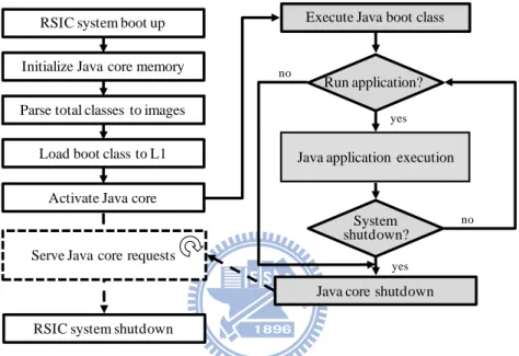
parses all class files and convert them into runtime information images and reserves all resolution information in the constant pool of the image. Fig. 2 shows the system life cycle of the previous platform. After system boot up, host RISC processor initializes system memory and parses all class files before execution. After all class files are parsed into information images, the system loads the boot class into Java method area and enables the Java execution engine.

Fig. 2. System life cycle of previous Java platform.

Fig. 3 describes the architecture of previous version of Java core [4]. The Java core execution engine is composed of four pipeline stages which fetch, translate, decode, and execute bytecode and micro-instructions. There are some issues with previous system which will be described later.

RSIC system boot up Initialize Java core memory Parse total classes to images

Load boot class to L1

Activate Java core

Run application?

System shutdown?

Java core shutdown RSIC system shutdown

yes

yes no

no

Serve Java core requests

Java application execution Execute Java boot class

Fig. 3. Previous Java execution engine [4].

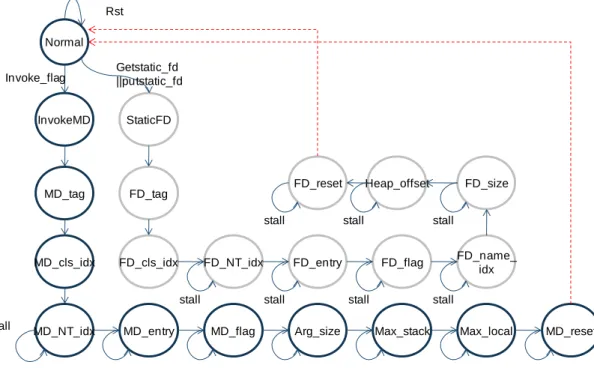
Some behaviors of Java bytecode are too complex for hard-wired implementation such as method invocation or field data access, etc. These behaviors require string resolution, which is too expensive for hardware execution. Previous design provides a dynamic resolution state machine to control the status of Java core execution engine. The main task of dynamic resolution controller is to handle symbol resolution of constant pool data. For example, the states of method invocation do resolution and get information which produced by class loader before execution as shown in Fig. 4. This state machine also controls and changes the program counter for referenced method bytecode.

Method Area Bytecode cache Management Unit _In iti a l P C

Bytecode Execution Engine

Execute Stage S ta c k D a ta st a ll a d d re ss wr d a ta rd d a ta pc B y te -c o d e s In te rr u p t External Memory Access Unit Translate Stage Fetch Stage Decode Stage T OS D at a R egs . Par am et er R egs .

Fig. 4. Original controller state machine for method invocation resolution. Finally, previous design does not reference to dynamic data information at run time and all essential information at runtime must be stored in runtime information image of a class. Previous design parses all class files before Java program execution. To make the Java SoC more flexible and stable, we redesign some subsystems and added the function of dynamic class loading. In chapter 4 I will present the design for dynamic class loading and discuss some additions to improve the Java execution engine.

2.2. 3-D MMI based on Stereo Cameras

2.2.1. 3-D and Image Coordinates Systems

We have presented the motivation of integration between the 3-D MMI and the proposed Java platform in chapter 1. A 3-D GUI system interacts with human operators‟ 3-D hand motions, captured by stereo cameras. The proposed MMI system computes the 3-D coordinates of the target object using the projection of the target

Normal Rst

InvokeMD StaticFD Invoke_flag Getstatic_fd_{||putstatic_fd}

MD_tag

MD_NT_idx

stall _{MD_entry MD_flag Arg_size Max_stack Max_local MD_reset} FD_tag

MD_cls_idx FD_cls_idx FD_NT_idx

stall FD_entry stall FD_flag stall FD_name_ idx stall FD_size stall Heap_offset stall FD_reset stall

camera intrinsic parameters such as effective focal length and sensor size, etc., and extrinsic parameters such as orientation and translation parameters. These parameters can be obtained by calibrating the camera using known landmark points. In this thesis, we use the camera calibration algorithm proposed by Tsai [15]. The camera model used here is the pinhole camera model. There are other camera models such as the orthographic projection model or the affine projection model.

Fig. 5. Pin-hole camera model.

Fig. 5 illustrates the pin-hole camera model. There are two 3-D coordinate systems shown in Fig. 5, the camera coordinate system and the world coordinate system. Traditional pinhole camera model converts the world coordinate system (WCS) into camera coordinate system (CCS) first, then projects 3-D objects to image plane and computes its 2-D positions w.r.t. image coordinates system (ICS) of the computer.

The first step in 3-D WCS to 2-D ICS projection is the rigid body transformation from (X, Y, Z) WCS to (X, Y, Z) CCS with 33 Rotation matrix R and 31 Translation

vector T. That is,

𝑋 𝑌 𝑍 𝐶𝐶𝑆 = 𝑹 ∗ 𝑋 𝑌 𝑍 𝑊𝐶𝑆 + 𝑻 (1) Cx Cy Cz Wx Wy Wz Pw( Xw , Yw , Zw ) / Pc( Xc , Yc , Zc ) Zc F Projection plane Pi( Xi , Yi)

𝑹 = 𝑟₁ 𝑟₂ 𝑟₃ 𝑟₄ 𝑟₅ 𝑟₆ 𝑟₇ 𝑟₈ 𝑟₉ 𝑻 = 𝑇_𝑥 𝑇𝑦 𝑇𝑧 (2)

The second step is to project the object, denoted in CCS, to ideal undistorted image coordinate (X, Y) Ideal using perspective projection of pinhole camera model as

follows:

𝑋_𝑖 = 𝑓 ∗ 𝑋𝑐

𝑍𝑐

(3)

The variable f is the focal length of the camera.

Thirdly, the effect of lens distortion is taken into account and compute the coordinate of image plane with lens distortion (X, Y) Distortion

𝑋_𝑑 + 𝐷_𝑥 = 𝑋_𝑢, 𝐷_𝑥 = 𝑋_𝑑 𝐾1𝑟2+ 𝐾2𝑟4 + ⋯ (4)

Fourth, we scale the image plain into computer image (X, Y) frame which is pixel

based frame image by some scale factor.

𝑋_𝑓 = 𝑆_𝑥𝑑_𝑥′−1𝑋_𝑑 + 𝐶_𝑥 𝑌_𝑓 = 𝑑_𝑥′−1𝑌_𝑑 + 𝐶_𝑦

𝑑_𝑥′ = 𝑑_𝑥 𝑁𝑐𝑥

𝑁𝑓𝑥 (5)

After below steps, the 3-D real objects are projected onto the 2-D image plane. We can adopt these images from different viewpoints to compute the 3-D coordinates through triangulation as shown in Fig. 6. Note that we need at least two views in order to perform triangulation.

Fig. 6. Compute original 3-D coordinate from two views.

The triangulation process requires camera parameters, which can be obtained through camera calibration. Next sub-section describes the basic concept of camera calibration.

2.2.2. Overview of Camera Calibration

Camera calibration can be divided into two categories. One is photogrammetric calibration and the other one is self-calibration. Basic photogrammetric calibration approaches use a camera to observe a set of known patterns called calibration landmark points and use the known 3-D to 2-D correspondence of these landmark points to calculate the camera parameters. Self-Calibration can calibrate the camera without any calibration landmark points [21]. Self-Calibration captures the static scene and generates image sequence by moving the camera. This technology estimates the calibration parameters from image sequence which captured by the same camera. The former is more accurate and more efficient then letter. But the former is also much more expensive. However the interaction interface between human and machine needs more reliable information especially for the motion of hand. There are also other approaches for specialized environment. We give an overview of another algorithm of photogrammetric calibration.

The camera calibration technology developed by Z. Zhang is also well-known [20]. This algorithm provides a flexible calibration process without specialized 3-D geometry. The camera only captures the planar pattern from anywhere. However some parameters such as lens distortion should be modeled. This calibration technology adopts a nonlinear approach based on the maximum likelihood criterion to solve the matrix derived from homograph between pattern and image. Even though technology of Z. Zhang is flexible and accurate, the calculation is too complex for embedded systems to do nonlinear optimization. Therefore, we adopts the camera calibration

algorithm by Tsai [15], which only use linear equations and general least square optimization which can easily be implement for embedded systems. The details of this algorithm will be presented in chapter 5.

Chapter 3. Overview of Java Processor

3.1. Overview

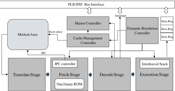
The dual-core Java application processor in this thesis is based on the architecture described in [2][4], which is a double-issue four-stage pipeline stack processor. The stages are Translate, Fetch, Decode, and Execute as shown in Fig. 7. The Java core also contains a method area and a cache management unit. Furthermore, Java core also supports three communication interfaces. One is the internal processor communication (IPC: interrupt) interface between RISC core and Java core. Java core request RISC for services through IPC interface. Another interface is bus master interface of Processor Local Bus (PLB v4.6). Java core can access other devices such as DDR memory through master bus interface. The third interface is a set of data registers. These data registers are used for information exchange with RISC processor. There is a thin kernel running on RISC processor and this kernel provides several services such as I/O, dynamic class loading or native function invocations. The IPC transmit function parameters to the RISC core through data registers and an interrupt service ID register. The system bus protocol is based on the Processor Local Bus (PLB) bus of the IBM CoreConnect bus [24]. The remaining sections of this chapter describe some details of the previous architecture. Some controller design and implementation flaws that lead to stable issues of existing Java core will also be discussed. The design and integration of dynamic class loading mechanism into existing architecture will be described in next chapter.

Fig. 7. Overall architecture of Java core.

3.2. Bytecode Execution Core

Fig. 7 shows the overall architecture of previous Java core. This Java core has a dynamic resolution controller unit which controls the status of Java core. Java core executes bytecode in normal mode. If a bytecode invokes dynamic resolution for data access in class runtime information image, the Java core will leave the normal mode and enters simple dynamic data resolution mode. The following sections describe the details for each component of Java core.

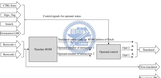
3.2.1. Translate Stage

This section describes the first stage of proposed pipeline architecture. Because the Java bytecode adopt variable code lengths and some bytecode behaviors are too complex to execute in one cycle, the proposed design achieves the same behavior of complex bytecode with simple instructions sequence. System separates the bytecode into two types in this stage. One type is one-to-one mapping type which the simple task can be done in one cycle. The other type is one-to-many mapping which complex task can only be done with a sequence of simple instructions. Simple type bytecode

Translate Stage Fetch Stage Decode Stage Execution Stage

Method Area One2many ROM Dynamic Resolution Controller Master Controller JPC controller JPC Cache Management Controller Ra m select Interrupt Interleaved Stack Da ta Reg Da ta Reg Da ta Reg

will directly be translated into one simple instruction for Java core. Then complex type bytecode will be translated into an ROM address mapping to an instruction sequence at Fetch stage.

This stage also determinates whether the bytecode are operands or not. If the bytecode are operands, these bytecode should not be translated and will be pushed into operands buffer at next stage. In order to follows double-issue, system fetch two bytecode at a time. Then system need to exactly know which one of the two bytecode should be executed, especially after jump, branch, and a data resolution for JPC variation. More details are described in [2].

Fig. 8. Architecture of translate stage.

CTRL State Stjpc_flag branch Destination LSB Translate ROM Bytecode 1 Bytecode 2

Translated micro code or ROM address of Fetch Operand number of instruction 1

Operand number of instruction 2 Operand control _{Opd 1} Opd 2 &

&

Translated

Non-translated

Pass restore JPC Control signals for operand status

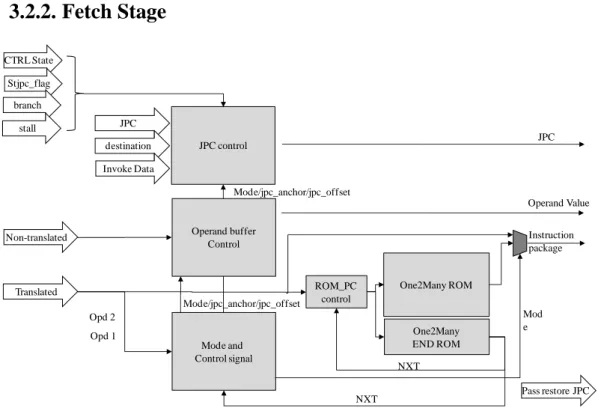
3.2.2. Fetch Stage

Fig. 9. Architecture of fetch stage

The Fetch stage is a most complex module as shown in Fig. 9. This stage has many important tasks such as Java core program counter (JPC) control, operands buffer control, and mode control (Complex bytecode execution mode/Simple bytecode execution mode), etc. Main purpose of Fetch stage is to generate correct instructions package for decode stage.

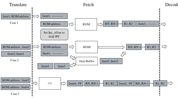
There are two cases of the instruction packages which transferred to Decode stage. First case, the bytecode of Translate stage is simple and the simple instructions package is obtained directly from former stage. Second case, the bytecode of Translate stage is complex bytecode and the instructions package is fetched from the one-to-many ROM by translated ROM address. Unfortunately, the former statge sometimes put the ROM address and the simple bytecode into the same package. Then the mode translation between passing simple bytecode or fetching bytecode from one-to-many ROM becomes a difficult problem as shown in Fig. 10.

Translated Non-translated CTRL State Stjpc_flag branch stall One2Many ROM ROM_PC control JPC control Operand buffer Control JPC destination Invoke Data Mode and Control signal Opd 1 Opd 2 One2Many END ROM NXT NXT Mode/jpc_anchor/jpc_offset Mode/jpc_anchor/jpc_offset Operand Value Mod e Instruction package JPC Pass restore JPC

Fig. 10. Some special conditions for instruction packages.

As Fig. 10 shows, this stage holds JPC in order to fetch instructions from One2Many ROM. At the same time, system also stalls the Translate stage for complex bytecode execution. System packages the instructions from ROM or directly from last stage at complex bytecode execution mode. Moreover, the packages from last stage also can be one or more operands. Finally, this stage should package instructions and operands correctly no matter for any combinations. This stage handles more JPC operations from above reasons, so we directly put JPC control module into Fetch stage.

3.2.3. Decode Stage

Decode stage generate control signals from instruction packages from Fetch stage. And the Fetch stage ensures all packages transferred to Decode stage which must be composed of only simple instructions. This stage would focus on generating appropriate data paths for different behaviors of instructions packages. In the beginning, system classes the data paths with instruction package types. The details and data paths of instructions pair types can be found in [2]. This stage not only generates the data path control signals but also picks correct value from immROM or

Fetch

Translate Decode

Instr1, ROM address Instr1,

---ROM address ROM

Set Jpc_offset to hold JPC

Instr1, ---R1, R2

RN, RN-1

ROM address , Instr2

Instr1,

---ROM address ROM RN, RN-1 R1, R2

Instr Buffer Instr3, Instr4

Instr3 Instr4

Instr2, Instr3

ROM address , Instr2

ROM address , Instr4

??? Instr4, FF RN, RN-1 R1, R2 Instr2, FF RN, RN-1 R1, R2 Case 1

Case 2

operands buffer for operations or stack access. The interrupt control module and bus data master access control module are also included in the stage. Some instructions like “new” or method invocation will invoke the interrupt signal at this stage. And the bus master access modules only control the target address and R/W request signal. The data transferred from the bus will handle at Execute stage.

Fig. 11. Architecture of decode stage.

3.2.4. Execute Stage

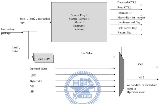
Fig. 12 shows the execute stage of the Java core. This stage is for the execution of ALU operations, stack operations, and external data accesses. The control signals of data paths control data sources, operations, multiplexers, and interleaved stack operations. The control signals of decode stage handle stack operation and stack pointers, where the interleaving stack structure makes things very complex for operations. The stack structure will be described in next section. Execute stage executes operations indicated by the control signal. Moreover, this stage has the critical path here from many levels of multiplexers and the multiply operations.

Special Flag / Control signals / Master / Interrupt / control Operand Value Instruction package JPC imm ROM imm ROM Bytecodes Instr1 , Instr2 , instruction type Instr1 , Instr2 ImmValue VP SP Val 1 Val 2

val : address or immediate value or Operation value Data path CTRL Read CTRL Interrupt ID Master Rd / Wr request

Field access flag Return flag Invoke method flag

Fig. 12. Architecture of execute stage.

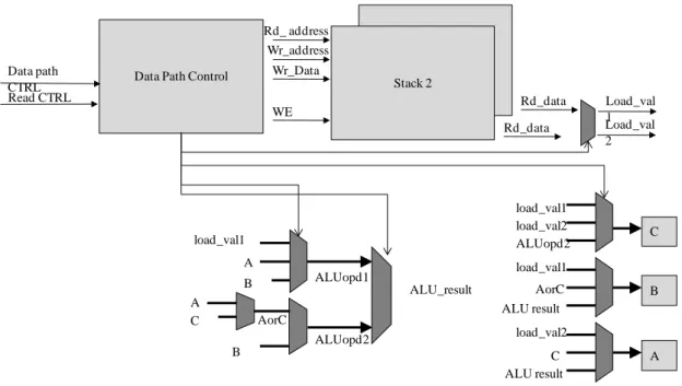
3.2.5. Stack Structure.

In this section, the interleaved stacks structure is resented, as shown in Fig. 13. In order to support double-issue, the stack memory is composed of two SRAM banks. And the two SRAM banks are interleaved together to enable simultaneous access of consecutive words of memory cells. All operations express with three top registers A, B, and C. The stack status can be expressed by two register SP and VP. The register SP is the stack pointer that points to the top of stack. The register VP points to the base address of local variables and arguments of current stack frame of the invoked method. The initial SP of each class should be placed after all local variables and method arguments from VP as shown in Fig. 13. The push and pop stack operations are described as follows.

 Push Operation: Load type instruction pushes data into top stack register

and the original data of bottom register C will be pushed back into the stack base on SP pointer.

 Pop Operation: Store type instruction or ALU operations pop data from Stack 1 Stack 2 Rd_ address Wr_address Wr_Data Rd_data WE Rd_data Load_val₁ Load_val 2 ALUopd1 A load_val1 B ALUopd2 B C A AorC ALU_result C load_val2 ALU result A load_val1 load_val2 ALUopd2 C load_val1 ALU result B AorC

Data Path Control Data path

CTRL Read CTRL

stack and store data back to the locals or still store to top registers.

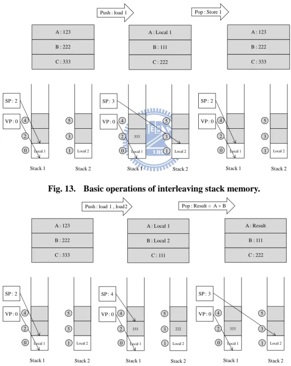
The concepts of the push and store operations are illustrated in Fig. 13 as well. The ALU operation is shown as Two loads and an ALU operation. If the numbers of top stack register are reduced, system needs pop data for SP pointer. We can just take the gray part as operand stack and the stack space between SP pointers and VP pointer stand for local variables or arguments.

Fig. 13. Basic operations of interleaving stack memory.

Fig. 14. Two loads and an ALU operation.

Stack 1 Stack 2 VP : 0 SP : 2 Local 1 Local 2 A : 123 B : 222 C : 333

Push : load 1 Pop : Store 1

0 1 2 3 4 5 Stack 1 Stack 2 VP : 0 SP : 3 333 Local 1 Local 2 A : Local 1 B : 111 C : 222 0 1 2 3 4 5 Stack 1 Stack 2 VP : 0 SP : 2 Local 1 Local 2 A : 123 B : 222 C : 333 0 1 2 3 4 5 Stack 1 Stack 2 VP : 0 SP : 2 Local 1 Local 2 A : 123 B : 222 C : 333

Push : load 1 , load2 Pop : Result = A + B

0 1 2 3 4 5 Stack 1 Stack 2 VP : 0 SP : 4 333 222 Local 1 Local 2 A : Local 1 B : Local 2 C : 111 0 1 2 3 4 5 Stack 1 Stack 2 VP : 0 SP : 3 333 Local 1 Local 2 A : Result B : 111 C : 222 0 1 2 3 4 5

3.3. Cache Management Unit

In this section, I will introduce the cache mechanism for existing Java core. As Fig. 7 shows, Java core fetch bytecode directly from method area. Previous method area has 32 2KBytes cache blocks. And the average size of standard Java system library is about 8 Kbytes, the method area is enough for usage. Then Java core manages the cache mechanism with a cache management unit. The cache management table contains the information of class runtime image such as the image size, the start address of external memory, etc. An entry of the table is shown in Table 1. This table is included in the cache management unit.

Table 1. Management Table of Cache Management Unit

When the Java core performs method invocation, it can query this table using the class global index. If the referenced class has been loaded into the method area, the Java core can adjust the JPC to the target method area from the start block index. This method area start index indicates the first cache block index of referenced class. On the other hand cache management mechanism loads referenced class from external memory by external memory start address field. Then the cache mechanism enters a loading loop for the referenced class image until data counter over the image size. This cache mechanism for class image loading is often invoked by method invocation which will be introduced in section 4.5.

Cache Manage Table

Global Index Tag Image Size 1st_{Cache Block}

Start Index

2st_{External Memory}

Chapter 4. Design of Java Dynamic Class

Loading Mechanism

This chapter presents the proposed dynamic class loading mechanism. We implement the proposed dynamic class loading mechanism with hardware-software codesigned method. This proposed mechanism is composed of two steps. We use software (executed by the RISC core) to parse the class files and collect runtime information. This software will generate a bytecode image with reference pointers and a cross reference table. The pointers in this image point to this table directly. The table contains all runtime information which collected from the original class file. This first step only executed by a new class loading event. After the system collect essential information, we can just apply second step to load the same class. Moreover, the second step is executed completely by hardware. Java core can resolve all runtime information with the reference pointer in bytecode image. This mechanism only has one-time class loader software execution overhead for each class throughout the life cycle of the JRE. When the same class is referenced for the second time, the Java core will simply transfer the previously created class runtime image from the external DDR SDRAM to the on-chip method area without any runtime class loading software overhead. An overview of the proposed dynamic class loading mechanism and the software class loader analysis will be presented in later sections. Details of dynamic resolution for method invocation and field data accesses will also be described in details. The detail descriptions of these mechanisms are also presented in later sections.

Mechanism

When a Java method invokes methods which belong to other class files, the referenced classes have to be loaded into the method area. Traditional JVM‟s have software dynamic class loaders to perform the class loading process triggered by method invocations. The dynamic class loaders perform complex dynamic data resolution identified by bytecode operands at first. The dynamic data resolution mechanism gets the class and method information by referencing the const pool data in class files. Then dynamic class loader must check the class method area to make sure whether the referenced class is in the method area or not. If the class is not in the method area, the dynamic class loader loads the class with a series of verification processes as Fig. 1 shows.

It is obvious that the traditional JVM‟s have high overhead for dynamic class loading. Even though the class is in the class method area, the JVM still have high overhead to do dynamic data resolution for runtime class information. Hence we propose a hardware-software co-designed dynamic class loading mechanism to deduce the overhead at runtime.

Fig. 15. Runtime dynamic class loading mechanism. Jar File System

2.Target Class

DDR – Image Space

3. Runtime Image ,

Image Information 5.Load target image _{with cache management}

Cross Reference Table

Image

Hardware

Java Core

RISC Core IPC

Java program execution Class Profiling Process

( Class Loader)

4.Return information

Our proposed hardware-software co-designed dynamic class loading mechanism has two steps. As Fig. 15 shows, when the Java program is executing at runtime and the program wants to do a method invocation from a different class. If the referenced class is invoked first time, Java core generates a “Load Class” event interrupt. Java core asks the RISC core to serve the “Load Class” request through IPC interface.

RISC core will perform the first step of proposed dynamic class loading mechanism in the proposed class loader. The detail analysis of class loader is in next section. This class loader will resolved the class path and class name of target class by querying the cross reference table with information from interrupt service. Then this class loader loads the target class from a Jar file system as the Fig. 15 shown.

This class loader continues to parse the referenced class file and generate the bytecode image and update our proposed cross reference table. Then cross reference table contains new information of referenced class. And the bytecode image also contains the reference pointers which point to these information fields of cross reference table. After the class loader collects essential runtime information of referenced class, RISC core responds to this “Class Load” interrupt service request with method invocation information. Java core enable our cache mechanism after the service returned. Then Java core follows cache mechanism and query cache management table by the returned method invocation. Finally, Java core can load referenced class from cache mechanism and the returned information.

When Java program wants to do method invocation and the referenced class has been loaded before, the Java core can access the cross reference table directly by the reference pointer in the bytecode image. Java core can get the same method invocation information as the information returned in the first step by accessing the

then Java core must enables cache mechanism to load the referenced class into the method area. The Java core can execute the method code directly if the referenced class is already in method area. The second step of the class loading mechanism only requires very simple hardware logic to implement. And it only requires one data bus transaction to retrieve the method invocation information. The overhead of repeated invocations of the same method is very small during runtime execution.

4.2. RISC-software of the Proposed Dynamic Class Loader

We introduce the software class loader which only executed in first step of proposed dynamic class loading mechanism. Proposed dynamic class loading mechanism construct the cross reference table by this class loader. This cross reference table provides all runtime information not only for method invocation but also other runtime data resolution. As the cross reference table has enough information for runtime execution, the Java core can reduce most overhead from the assistance of this table.

Fig. 16. Overview for the flow of class loader

In this section, we introduce this class loader process and the software overhead analysis. The Fig. 16 describes the general flow of proposed class loader process. The Java core invokes the RISC core service with referenced class global index. The global index of referenced class is allocated at the loading time of the running class. We can make sure the referenced class has registered in advance. The cross reference table already has registered the name of referenced class, but without other details information. Then RISC core get the referenced class name and class path by querying cross reference table with global index.

The function “Jar file system open “will find the referenced class file through the class path in Jar file system at first. Then this process also invokes the class loader process to generate the bytecode image and update the cross reference table. As the Fig. 16 shows, class loader first resolve the const pool of class file and get the information of method reference and field reference in this referenced class. The

RISC service – Class Loading Mechanism Class Loader

Jar file system open() Query the cross reference

table by global index and

get load class name Parse Const Pool Management of Referenced

Information , resolution of referenced pointer Resolution of field data Information and update the

cross reference table Resolution of method data Information and update the

cross reference table Service Return

another class. Then we also get reference pointer for this class to reference other classes. Then class loader continues to resolve method data and field data of this loading class. Finally the cross reference table gets the method information from loading class (referenced class by running class). Then the service returns this information to the Java core and completes the onetime cost class loader process.

We can find pseudo-code and total operations count in Appendix section. The operations count depends on the total registered classes‟ number, method count of each registered class and field count of each registered class. If the complexity of method or field reference increases, the cost of software also increases. There are still a lot of acceleration issues for software class loader optimization.

4.3. Cross Reference Table with Memory Management

The cross reference table plays an important role of the dynamic class loading form section 4.1. Our proposed Java Runtime Environment registers information such as class or method or field data information to this cross reference table by profiling class file as shown in section 4.2. The cross reference table not only helps runtime resolution to the dynamic class loading mechanism, but also gives helps to method invocation and field data access and memory management. A typical cross reference table with all features is shown in Table 2.

Table 2. Cross Reference Table with Data Field Features

Table 2 shows all information registered on the table fields for one class. When class loader parses a new class, the loader allocates a new global index and creates a

Cross reference table

Class [x]

Attributes Class name, global index, image address, parent class index Method[i] Name Global index & method1 offset

table space for new class. Basic table field includes class name, class path name, image start address of external memory, and image size. If the class is load yet, the cross reference table still has registered from other class would reference to it. When the class loader gets a loading class event with global index; the loader can query the table by global index to get the non-load class name. And class loader can find load correct class file from correct Jar file path [8].

The method invocation is the only behavior would invoke the “Load class event.” Java core will invoke the interrupt service when the method invocation references to a new class. When the class has been loaded, Java core can directly accesses expected information for usage. And the field data access mechanism also can be a fast hardware mechanism. The sections 4.5 and 4.6 describe how Java core use the information of cross reference table to do method invocation and field data access. Section 4.4 shows current runtime image and how to do the dynamic resolution to their information.

4.4. Runtime Image Format and Resolution

Fig. 17. Image format and memory allocation.

Fig. 17 shows the runtime memory allocation for Java environment and the gray region is the runtime image and its format. This image format can be divided into five parts. The first part contains the image header and numbers of information data and reference information. The second part is TOC offset table, and every entry of this table is two bytes. The TOC offset entries indicate the byte length from image‟s head to the resolution information data. The Java Core can directly jump to correct address for data resolution by TOC offset entries in this table. The third part is purely char arrays. The fourth part describes all reference resolution information and address links to the cross reference table of section 4.3. For example, method reference information field contains the method owner class‟s global index. And fields of name index and

(8 bytes) --- MMES , Const Pool Numbers TOC Offset

(2 Bytes offsets each entry)

Char array

( 2 Bytes Length , Length * Bytes )

Field / Method Reference information (2 bytes , 2bytes , 2 bytes , 4 bytes)

Global index Name index1 descriptor Cross address Global index Name index1 descriptor Cross address

Method Code Data

(2 bytes , 2bytes , 2 bytes , 2 bytes, N-Bytes Code) Global index # of Argument Max stack Max local

Method Code

Global index # of Argument Max stack Max local Method Code

Char Length Chars ….. Char Length Chars …..

Offset Offset DDR Memory Cross Reference Table L2 Method Area Heap memory

descriptor both are TOC index for their char arrays. The cross address fields are most important of all information. This field points to the cross reference table field address with method offset for method invocation or physical field data address. The method offset mean the byte length from image head to method bytecode section. The last part is method code data. The bytecode, arguments numbers, local variable numbers, and max stack numbers all have stored in this part for Java core execution.

4.5. Method Invocation Mechanism

This section introduces the method invocation mechanism of the Java core. There are two types of Java method invocations. One is static class method invocation and the other one is dynamic instance method invocation. Static method invocation such as invokestatic references to class method directly. Dynamic method invocation such as invokevirtual and invokespecial depend on their object references. Nevertheless, the proposed Java core executes them with the same procedure. The proposed class loader recognizes these method invocation types and inserts special parameters to indicate the object reference at parsing time. Moreover the invokespecial can be used under three conditions. First, the method is used for instance initialization. Second, the method is a private method. Third, the method is invoked from a “Super” keyword. Current version can support bytecode such as invokestatic, invokespecial, and invokevirtual. The complete method invocation procedure can be described by the state machine in Fig. 18. In a normal class file, a method invocation bytecode is followed by the class and method reference ID‟s of the class name string and method name string that are used for computing the target address of the method. With the proposed dynamic resolution mechanism, the invocation bytecode in the class runtime image (translated by the class loader) is

Fig. 19 illustrates how the operand can be used to access the target method address through indirect references. There is no need to perform any string comparisons as in traditional JVM dynamic resolution process..

Fig. 18. State machine of method invocation mechanism.

Fig. 19. Method invocation resolution steps.

Fig. 18 describes the state machine of method invocation mechanism. The state Normal Rst Invoke_flag Get entry (1) (2) Up address stall (2) Low address (3)Offset access Bad(4) Index (5)Enable Method manager

Arg_size Max_stack Max_local MD_reset Master trigger (6) MD_entry Type 1,2 Type 3 stall

Type 1 : The class which contains this class had been parsed and place in the external DDR Memory

Type 2 : The class had been parsed and place in the Internal Method Area Cache

Type 3 : Need interrupt to load and parse class from jar file store at CF Card

Image File Start

TOC

Const Pool Data

Method Code Space

(1) Method informa tion , cross table field address

Offset to const pool da ta

(2)

(3)

(4) : No

Image File Start

TOC

Const Pool Data

Method Code Space (6)

Cross Reference Ta ble Access

Hardware Java Core Invoke + opera nd (Toc index ma pping)

Cla ss ma na ge Logic Circuit Decision Logic : Cla ss ha d been loa ded or not ?

Interrupt Cla ss (4) Loa ding service

DDR External Memory

Cross Reference Ta ble

(5) (5):Loa ded

machine is controlled by dynamic resolution controller of Java core. The method invocation mechanism can be divided into four stages roughly. Java core can find referenced class and referenced method bytecode information by following this state machine.

Fig. 20. Reference pointer and method information access

The first stage of method invocation state machine is to find the reference pointer in bytecode image. The first 4 states of state machine are the first stage. Java core will exchange the program counter to obtain the reference pointer from these four stages.

The second stage will access the cross reference table by reference pointer from first stage. And the method invocation state machine performs this behavior at “Offset access” state. As the Fig. 20 shown, the field of cross reference table referenced is a 32-bits data field. The up 16-bits of this field indicate the referenced class‟s global index. The low 16-bits of this field indicate the method offset of referenced method. The method offset stands for the method bytecode address offset of its bytecode image. In this stage we can judge whether this referenced class has ever loaded or not by the method offset. If the referenced method has correct method offset, we can

Image File Start

TOC

Const Pool Data

Method Code Space Method [i] informa tion , Reference Pointer

Offset to const pool da ta

Access Cross Reference Table

Cross reference table

Class [x]

Attributes Class name, global index, image address, etc

Method[i] Name Global index & method1 offset

referenced class which not loaded before, Java core enters the bad index and waits for the RISC core service as above sections. The Java core enters the third stage until the RISC service finish. If the referenced class has loaded before, the Java core enters third stage directly.

Fig. 21. The cache mechanism of third stage

Java core will get sufficient method information from RISC core service or cross reference table. The third stage enables our bytecode cache mechanism. Java core can query the cache table by the global index which is upper bits of method information field. The Java core follows the cache mechanism and checks method area cache block index at first. If the referenced class has allocated to method area, the cache table will register the start block index. If the referenced class has not allocated to method area, Java core can load its bytecode image with other information such as start address in external memory and the image size.

Cache Management Table In Java Core Global Index Tag Image Size 1st_{Cache Block}

Start Index 2st_{External Memory} Start Address Wait enable enable = 0 enable = 1 Check block index Ready Image loading Update block index Counter > Image Size

Fig. 22. Adjust Java core to access referenced method bytecode

After the referenced class has loaded into method area, Java core adjust its stack frame and program counter as the Fig. 22 shown. The method offset from cross reference table helps the Java core to update program counter. Then Java core continues to execute new method as usual.

Then this final section continuously describes the stack status during method invocation mechanism. The Fig. 23 describes the stack status of method invocation which the method invoked has two local variables and no argument. The Fig. 24 is also the method invocation with one argument and two local variables. The Fig. 25 and Fig. 26 are then method return which one is “Void return” and another is “Integer return.” Block 1 Block 2 Block 3 Block 4 Block 32 Image 1 Image 2 Empty

Block index & Method Offset

Java Program Counter

Bytecode start address of referenced method

Method Bytecode

Fig. 23. Method invocation stack variation – no arguments, 2 local variables.

Fig. 24. Method invocation stack variation – 1 argument, 2 locals. Stack 1 Stack 2 VP SP Local 1 Local 2 A : 123 B : 222 C : 333 Load reserved , JPC , VP Stack 1 Stack 2 A : VP (0) B : JPC C : Reserved

Update VP ,SP ,next class with 2 locals

Stack 1 Stack 2 111 VP SP 333 222 Local 1 Local 2 A : VP (0) B : JPC C : Reserved 111 Nlocal 2 New VP New SP 333 222 Local 1 Local 2 NLocal 1 Stack 1 Stack 2 VP SP 333 Local 1 Local 2 A : arg1 B : 123 C : 222 Load reserved , JPC , VP Stack 1 Stack 2 A : VP (0) B : JPC C : Reserved

Update VP ,SP ,next class with 2 locals

Stack 1 Stack 2 111 arg1 VP SP 333 222 Local 1 Local 2 A : VP (0) B : JPC C : Reserved 111 arg1 VP SP 333 222 Local 1 Local 2 Nlocal 2

Fig. 25. Method invocation stack variation – Method Return without value (void).

Fig. 26. Method Invocation Stack Variation – Method Return with value “ireturn.” Stack 1 Stack 2 A : VP (0) B : JPC C : Reserved 111 arg1 VP SP 333 222 Local 1 Local 2 Nlocal 2

Restored VP , SP = VP -1 Restored JPC to Last Method , 1 POP

Stack 1 Stack 2 A : JPC B : Reserved C : 111 VP SP 333 222 Local 1 Local 2 Stack 1 Stack 2 A : 111 B : 222 C : 333 VP SP Local 1 Local 2 Local1 Local2 Stack 1 Stack 2 VP SP LLast JPC LLast VP Reserved …… A : Last VP B : La st JPC C : Reserved

Load return value

Local1 Local2 Stack 1 Stack 2 VP SP LLast JPC LLast VP Reserved …… A : Return value B : La st VP C : La st JPC Reserved 0x73 : store_return Local1 Local2 Stack 1 Stack 2 VP SP LLast JPC LLast VP Reserved …… A : Last VP B : La st JPC C : Return va lue Reserved

4.6. Field Data Access Mechanism

Fig. 27. Dynamic resolution state for field access mechanism.

The field access mechanism is somewhat like the method invocation mechanism. The state machine is also controlled by dynamic resolution controller. The Fig. 27 is the dynamic resolution state transaction flow for field data access, and the first three states are also for the reference pointer mapping. After Java core get the reference pointer, this field of table should contain a pointer of physical memory address for static field data or a variable order index for non-static variable. In the case of non-static variable, the Java core will calculate correct memory address of heap memory by object reference address of heap memory and the order index. The Fig. 28 describes a complete flow for non-static variable access.

Normal Rst field_flag (1) FD_start (2)Up address (2)Low address Offset access Field access ( Read ) Master trigger FD_exit Field access (Write) stall stall stall

Fig. 28. Step flow for field data access mechanism.

Static field access mechanism has only one thing different form non-static. The cross reference table field has different meaning between static and non-static. In the static case, this field describes a physical memory address for static value which follows the image space, but order index for non-static field access.

Image File Start

TOC

Const Pool Data

Method Code Space

(1)

Method informa tion , cross table field address

Offset to const pool da ta (3)

(4) : No Cross Reference Ta ble Access

Hardware Java Core

Field a ccess + opera nd (Toc index ma pping)

Access field da ta (5) Get non-sta tic informa tion or

Sta tic a ddress

DDR External Memory

Cross Reference Ta ble

(2)

Field Da ta Spa ce Ca lcula tion of correct field

Chapter 5. Camera Calibration

We presented basic concepts and some technologies of camera calibration process in Chapter 2. Then we chose calibration algorithm of Roger Tsai which is suitable for our proposed embedded Java platform. We continue to describe the details of our implementation of Roger Tsai‟s algorithm in this chapter. We verify our implementation with a virtual simulation environment. The virtual simulation environment is set by Blender Tool 2.49. This chapter describes the usage of Blender Tool at first. Then following section describes the image process for abstracting the orientation of landmark points from image. The final section describes the implementation of calibration process.

5.1. Camera Calibration Algorithm

In this section, we will describe the camera calibration algorithm by Tsai [15].

5.1.1. Calibration Algorithm

Fig. 29. Perspective Projection Model with Lens Distortion

This section introduces the motivation and basic concept of Roger Tsai‟s camera calibration algorithm. Main concept of this algorithm is to calibrate the camera by linear equation derived from the physical property of optics. And this algorithm can

O X Y P Z Pu Pd Oi Poz

be divided into two parts. All calculation of this algorithm do not involved non-linear optimization, there is only linear problem need be solved. The one is to compute 3-D orientation position parameters. Another is to compute effective focal length, distortion coefficients, z-position and scale factor which more camera intrinsic parameters. The following sections describe the detail of two parts individually.

5.1.2. Computation of 3-D Orientation Position Parameters

We introduce first step in this section. We observe the Fig. 29 at first. The line segments OiPd, PozP, OiPu is parallel each other because of the Radial Alignment

Constraint (RAC). Then we can find the vector (X d, Y d) of Pd and the vector (X, Y)

of P are also parallel each other. And we also conclude the outer product of these two vectors is zero. Then we can derive an equation from (1).

𝑋_𝑑𝑌_𝑐𝑐𝑠 − 𝑌_𝑑𝑋_𝑐𝑐𝑠 = 0 (5)

𝑋_𝑑 𝑟₄𝑋_𝑤 + 𝑟₅𝑌_𝑤 + 𝑟₆𝑍_𝑤 + 𝑇_𝑦 − 𝑌_𝑑 𝑟1𝑋𝑤 + 𝑟2𝑌𝑤 + 𝑟3𝑍𝑤 + 𝑇𝑥 = 0 (6)

Finally we derive (5) from (1) and (2). Then we can rearrange the variables to five unknowns because of Zw to be zero for coplanar calibration system or

non-coplanar calibration system. Moreover the Xd, Yd variables are available from (3).

The model of coplanar or non-coplanar are introduced at next section. Then we can conclude two linear systems for different calibration landmark point models. We can get parameters of rotation and translation matrices from these linear systems with known position of landmark points. Equation (7) is for non-coplanar model and Equation (8) is for co-planar model.

𝑌𝑑𝑖𝑥𝑤𝑖 𝑌𝑑𝑖𝑦𝑤𝑖 𝑌𝑑𝑖𝑧𝑤𝑖 𝑌𝑑𝑖 − 𝑋𝑑𝑖𝑥𝑤𝑖 − 𝑋𝑑𝑖𝑦𝑤𝑖 − 𝑌𝑑𝑖𝑧𝑤𝑖 𝑇𝑦−1𝑧𝑥𝑟1 𝑇_𝑦−1_𝑧 𝑥𝑟2 𝑇𝑦−1𝑧𝑥𝑟3 𝑇_𝑦−1_𝑧 𝑥𝑇𝑥 𝑇_𝑦−1_𝑟 4 𝑇𝑦−1𝑟5 𝑇_𝑦−1_𝑟 6 = 𝑋𝑑𝑖 (7) 𝑌_𝑑𝑖𝑥_𝑤𝑖 𝑌_𝑑𝑖𝑦_𝑤𝑖 𝑌_𝑑𝑖 − 𝑋_𝑑𝑖𝑥_𝑤𝑖 − 𝑋_𝑑𝑖𝑦_𝑤𝑖 𝑇_𝑦−1_𝑟 1 𝑇𝑦−1𝑟2 𝑇_𝑦−1_𝑇 𝑥 𝑇𝑦−1𝑟4 𝑇_𝑦−1_𝑟 5 = 𝑋_𝑑𝑖 (8)

5.1.3. Computation of Effective Focal Length, Len Distortion,

Z-Position

After first stage computation we can estimate three rotation angles parameters, translation of x-axle and y-axle and scale factor in this stage. The second stage computes remain parameters as the title 2.4.1. From relating (3), (4), and (5) we can estimate the z-axle of translation matrix and the effective focal length by (9).

𝑑_𝑦 ∗ (𝑌_𝑓− 𝐶_𝑦) = 𝑓 𝑟4𝑋𝑤 + 𝑟5𝑌𝑤 + 𝑇𝑦 _𝑟

7𝑋𝑤 + 𝑟8𝑌𝑤 + 𝑇𝑧 (9)

Then we get approximations of focal length and z-axle by ignoring lens distortion from (9). This over-determined system of linear equation can be solved easily from least square method. Finally we compute exact values of focal length, z-axle and lens distortion and use the result of last computation as initial guess for standard optimization of(9). The (10) is also derived from (3), (4), and (5). And we can select some standard schemes such as Steepest descent, Newton method or Powell method for standard optimization. After this calibration algorithm we can get all essential parameters for computing the coordinates of 3-D object.