修正的景氣循環過濾設計與其台灣總體經濟變數的應用

行政院國家科學委員會專題研究計畫成果報告

修正的實質景氣循環過濾設計與其台灣總體經濟變數的應用

Modified Filters in Real Business Cycle and

Applications to Taiwan Macroeconomics Variables

計畫別類： 個別型計畫 整合型計畫 計畫編號： NSC 87-2415-H-002-005 執行期間： 民 86 年 8 月 1 日至 民 87 年 7 月 31 日 個別型計畫：計畫主持人：林建甫 共同主持人： 整合型計畫：總計畫主持人： 子計畫主持人： 註：整合型計畫總報告與子計畫成果報告請分開編印各成一冊，彙整一 起繳送國科會。 處理方式： 可立即對外提供參考 (請打 X) 一年後可立即對外提供參考 兩年後可立即對外提供參考 (必要時，本會得延展發表時限) 執行單位： 台灣大學經濟學系 中華民國： 88 年 3 月 1 日

Modified Filters in Real Business Cycle and Applications to Taiwan Macroeconomics Variables

Chien-Fu Jeff Lin

Department of Economics, National Taiwan University

March 1999

Abstract

In this project, I study the growth and cyclical components of Taiwan macroeconomics variables by modifying filters recently used in real business cycles literature. A distinct feature of the new classical and modern real business cycle theories is to view the growth, business cycles and seasonal variations in a unified equilibrium framework. To assess the performance of the economy, they still need to decompose the series into growth and cyclical components. The way to separate the series is often applying some filters in the model. However, if there exist large exogenous shocks which are beyond the rational expectation of the economic agents, the filters in terms of backward and forward moving averages will be strongly affected by the shocks. The decomposition between the growth and cyclical components will become spurious. I compare the decomposition by the traditional design of the filters and my modification which includes the dummy variables to illuminate the large exogenous shocks. I identify the real part of growth and cyclical components in our macroeconomic variables. And then proceed to study the periodicity, comovement and relative volatility between variables. The data I used is from DGBAS which is the original data without any seasonal adjustment. From the pattern of the series, there do show some big shocks. This provides a good experiment to test the original filters and modified filters. Finally I address the questions often asked by the real business cycle. I find the declining of productivity growth in the economy is not true. But the consumption relative smooth then investment is indeed true.

________________________________________

*Research for this study was supported by a grant from the ROC National Science Council (Grant number: NSC 87-2415-H-002-005).

中文摘要， 在這一個研究中，我研究台灣總體經濟變數的成長部份及循環部份。我使用的 方法將是應用現在流行的實質景氣循環的文獻所使用的方法。但我將同時使用其 所用的過濾設計，也修改其過濾設計。藉此我們可以更了解台灣總體經濟變數真 正的成長部份及循環部份。雖然新古典及實質景氣循環學派的一個重要特性是將 成長部份，波動及循環部份一起以一個均衡的角度來研究。但為了獲得經濟體系 的表現，也需要將資料藉由過濾設計萃取其中的成長部份及循環部份。可是其所 使用的過濾設計，將深受外生巨大噪音或衝擊的影響。尤其是將其寫為前推及後 移的移動平均則此噪音將影響前後數期。那麼所區分的成長部份及循環部份及後 續的研究也就相當有可疑之處。我比較傳統的過濾設計及簡單修正加入虛擬變數 的過濾設計來消除巨大的或超過理性預期之下的衝擊。由此來了解台灣總體經濟 變數真正的成長部份及循環部份。我也探討了變數的循環性，共同震動性，及相 對的波動性。因為我所使用的資料是主計處的季資料，它並沒有經季節的調整， 所以一些特別大的噪音特別明顯，這更提供我使用修正的過濾設計的基礎。我的 研究回答了一般實質景氣循環理論者常問的問題：台灣的經濟成長沒有巨幅衰退 的嚴重性，可是台灣的消費相對穩定於投資的變動。這與世界主要國家的研究結 果是相同的。

1. Intr oduction

The first 25 years following the end of the second world war were halcyon days of Keynesian macroeconomics. The main policy implication was the government can fine-tune the economy by policies, especially fiscal policy. The study of business cycle

theory became not necessary. For example, in Bronfenbrenner (1969), he asked “Is the

Business Cycle Obsolete” in the title of his book? Although the acceleration and multiplier effects in the model did create fluctuations in the economy, serious depressions and booms can be avoid and remove from the economy by the correct economic policy. However, during the 1970s, the energy crisis gave a rebirth of interest in business cycle research. High inflation with high unemployment led economics to pay attention to the theory of monetary economy and expectation of the agents.

The dominant new classical theory during the period 1972-1982 was the monetary surprise model. The model was also a hallmark to explain the business cycle theory. It included a supply function developed by Lucas (Lucas 1972, 1973) using the structure of information set available to the producers. Sargent and Wallace (1975, 1976) combined the supply function with the Friedman-Phelps natural rate hypothesis and the assumptions of continuous market clearing and the rational expectation hypothesis to demonstrate a policy ineffective proposition. The inflation is governed by the rate of monetary expansion and because of rational expectations in agents’ mind, they cannot be systematically surprised, then anticipated monetary policy will be ineffective. This proposition implied only the surprise matters, a short run Phillips curve would result if inflation was unanticipated. This gave a explanation of the business cycle.

However, such models had also reached both a theoretical and an empirical difficulty by 1982. The sticky prices challenged the information confusion which gave a problem of money to output causality. Sims (1980) doubted the causal role of money in money-output correlation. Barro (1993) showed the anticipated money did not give a robust neutrality. To use the monetary surprise model to explain the business cycle has come to an impasse. Besides, economists became more involved with the statistical properties of economic time series. Time series data in the economics often show an upward trend. Nelson and Plosser (1982) tested major macro time series in US and could not reject the unit root hypothesis. This challenged the conventional wisdom. Traditionally economist adapted the idea that long run component follows a deterministic trend, the short run components fluctuate around the trend. The long run

component reflects the trend rate of growth generated by neoclassical growth model (Solow, 1956). The short run fluctuations are from the aggregate demand shocks. The finding in Nelson and Plosser (1982) that the economic series are difference stationary and not trend stationary or trend reverting show the impact of shocks have long run or permanent effect and not just short run or transitory effect. This conferred the rise of real business cycle school and emphasis on the supply shocks in the economy.

A distinct feature of the new classical and modern real business cycle theories is to view the growth, business cycles and seasonal variations in a unified equilibrium framework. Frish (1933) distinguished the impulse and propagation mechanism in the business cycles. The traditional Solow neoclassical growth model postulates the growth of output per worker over a long periods which depends on a smooth technological progress. However, real business cycle theorist reject this view and emphasize the erratic nature of technological change which they regards as the major cause of changes in aggregate output.

Real business cycle theorists also questioned the stylized facts of the economy. Traditionally, Keynesian and monetarist theorists thought the aggregate demand disturbances drive the business cycle, the real wage in counter-cyclical. However, Keyland and Prescott (1990) found that real wage behaves in a “reasonably strong” procyclical manner. It is a finding consistent of the shift of product function. The procyclical behavior of general price level is a fundamental feature of keynesian, monetarist and the monetary misperception version of new classical model. Keyland and Prescott (1990) also found that, in the USA during 1954-89, “the price level has displayed a counter-cyclical pattern”. Therefore the stylized facts become vague and controversial. A major concern in real business cycle theorists is the shift of the technology which leads this interesting result. I think this is especially important in the high growth economy like Taiwan.

Business cycle theorist are often interested in periodicity, comovement and relative volatility, e.g. Lucas (1987), Prescott (1986). To investigate those problem, they need to decompose the series into growth and cyclical components. The way to separate the series is often applying some filters in the model. Kydland and Prescott (1982) used the filter in Hodrick and Prescott (1980), (HP filter) to discuss the “Time to Build” phenomena. The HP filter can be written as a two side symmetric moving average filter. Singleton (1988) shows it is like a high pass filter when applied to a stationary series. King and Rebelo (1993) showed that HP filters can transform series which are integrated up to order 4 into stationary and it can be viewed as a generalized

exponential smoothing filter. Cogley and Nason (1995) found HP filter can generate spurious business cycle even if there are none in the original data. They also extended Sigleton’s result into time trend stationary data and derived the effect on difference stationary data. The effect is equivalent to a two step filter: difference the data to make stationary and then smooth the differenced data with an asymmetric moving average filter. However, the smoothing operation can amplify growth cycles at business cycle frequencies and damps long and short run fluctuations. In Nelson and Kang (1981), they showed that a detrend random walk exhibits spurious cycle effects whose average length is roughly two thirds of the sample length which become an important transitory shocks.

Baxter and King (1995) listed five properties that a good filter should have. First, the filter should extract a specific range of periodicity, and otherwise leave the properties of this extracted component unaffected. Second, the filter should not introduce phase shift. Third, the filter can approximate ideal band pass filter and we can measure the loss function for discrepancies between exact and approximate filter. Forth, the filter can results in a stationary time series even when applied to trending data which includes different orders deterministic trend and stochastic trend. Fifth, the filter should yield business cycle movements which is not subject to the length of sample period. Sixth, the filter is easy to operate. Therefore Baxter and King (1995) proposed a set of approximate band pass filters designed for use in a wide range of economic applications.

However all the consideration above did not think a big exogenous shock have important effects in the filters. If there exist large exogenous shocks which are beyond the rational expectation of the economic agents, the filters in terms of backward and forward moving averages will be strongly affected by the shocks. The decomposition between the growth and cyclical components will become spurious. I will compare the decomposition by the traditional design of the filters and my modification which includes the dummy variables to illuminate the large exogenous shocks. I hope to identify the real part of growth and cyclical components in our macroeconomic variables. And then proceed to study the periodicity, comovement and relative volatility between variables.

The quarterly data I used is from the directorate-General of Budget, Accounting, and Statistics (DGBAS) office in Taiwan. The range is from 1966:1 to 1995:2 which consisting of 118 time series observations for each variable. The data set contains some real variables and some nominal variables with price deflators. Consumption is

considered by food consumption CF and nonfood consumption CO. Income is used by the potential GDP, denoted as QF; the industrial product GDPIND; the gross national product GNP and the nominal GNP, denoted as GNPN. The private wealth is represented by quasi money MQM which consists mainly of the short term asset demand of bank deposit and short term bill issued by the central bank. Foreign reserve is represented by AFRN. The production side we utilize the existing capital stock K88 which is one period of the time lag and the private fixed investment, IBF. We also consider the international trade sector because it is important in the Taiwan economy. The total import value TVM and the total export value TVX. For the price deflator, we chose the consumer price index, CPI, the wholesale price index, WPI and factor income from the abroad price deflator, PFIA.

All the series are seasonal unadjusted. We can see some seasonal pattern in Figure 1. If the series are detrended by a regular difference, the seasonal pattern will be much clear. From the pattern of the series, there also show some big shocks. This provides a good experiment to test the original filters and modified filters.

I want to address the questions often asked by the real business cycle theorists. Is the productivity growth seriously declining in our economy? Is the consumption relative smooth then investment in our economy? Are the nominal and real wage and the general price level pro-cyclical or counter cyclical in our economy? And how much percent of the variation in productivity can be explained by the changes of the Solow residual in our economy? Because the GNP growth rates slow down during these years, part of the reason is due to the political upheaveal which disrupts the existing performance and structural of our economy. However, if we apply the modified fileters into our economy, we might have a clear picture what is the real growth component and cyclical component in our economy. We also can understand the comovement of our macroeconomic variables. To know the pattern of real and nominal wage, general price level with the business cycle path will give economic authority policy advise. And knowing how much percent of the variation in productivity can be explained by the changes of the Solow residual in our economy can help us to identify and measure the rate of technological progress.

The paper is divided into five parts. The first one is this introduction. The second section provides the object and model. The third section discusses the method in practice. The fourth section is the empirical part , and the conclusion is in the final section.

2. The Object and the model

Our object is to describe the picture of our business cycle, investigate the growth and cyclical component in our major macroeconomic variables and study their relationships.

The comparison of the filter mechanism are based on the filtered results. Traditional real business cycle emphasis on the comovement and correlations of the variables. Here we also include the usual criterion from model selections in econometrics. We will use AIC, BIC, SBIC as the supplement index to view the adequacy of the model.

The methods to decompose a time series between growth and cyclical component are related to the studies of business cycles. I summaried the methods in thre catogories, the naive filters, the pass filters and derived filters. The Naive method, we mean the easiest and intuitive way to implement. They should includes detremnistic detrend, linear stochastic detrend and moving average. The linear detremnistic detrend follows the conventional wisdom to regress the series against a deterministic trend and model the rest by an ARMA model. The linear stochastic detrend uses the regular difference and seasonal difference to detrend and also model the rest as the by an ARMA model. The moving average need symmetric coefficients to reach a trend reduction, see Baxter and King (1995). The pass filters which include low pass filter (the high pass filter) and band pass filter are established from the statistical point of view to

eliminate the specific frequencies. The derived filters are calculated from some specific objective function.

The studies are not only concentrating in the time domain but also on the frequency. Because we often use the Fourier transfor of the series, computing the periodic components associated with a finite number of “harmonic” frequencies. And then it is easy to see the frequencies which are removed or amplified. Besides, it is more natural to think in terms of periodicity of the cycles than frequencies. The periodic components are orthogonal to each other, therefore, it is easy to see the variance of the series as the sum of all the spectral density at different frequency.

The mathematical expressions are the following. The basic model we considered is the following

y_t =y_tg +y_tc +D_ti +ε_t

where y_tg is the growth component, y_tc is the cyclical component, D_ti is the

0.

(a) Naive method:

Linear detremnistic detrend

y_t = + +a bt D_ti +ε1_t, where ε1t follows ARMA Process. Therefore we

define y_tg = +a bt , y_tc =ε1_t

Linear stochastic detrend

y_t =y_t−1 +D_ti +ε , where ε2_t 2t follows ARMA Process. Therefore we define

y_tg y t = ₋1, yt c t =ε2 Moving average y_tg a L y_t a y j J j t j = ( ) =

∑

3. The Method in Pr actice

In this section we provide the model in practice, we decompose it into the pass filter and the derived filters. First, let’s look at the pass filter.

The low pass filter is the building block of pass filter, by which we mean a filter retains only slow-moving components of the data. The ideal low-pass filter has a

frequency response function given by β ω( )=1 for | |ω ω≤ and β ω( )=0 for

| |ω ω> . We need to apply the inverse Fourier transform to the frequency response

function to produce the time domain representation

b_{h =} ei hd −

∫

∑

However an infinite-order moving average is necessary to construct the ideal filter. In, practe, we need to trancate the lags in the moving average. The filter we considered is

constructed by simply elimilate the lag length at K. Following Baster and King (1995),

we use LP_K ( ) to denote the low pass filter which is trancated at lag K and whichp

passes components of the data with periodidity greater than or equal to p. Then we

(a) The low pass filter as LP_K ( ) =b(L).p y_tg b L y b y t _{k K} K k t k = ( ) =

∑

(c) The band pass filter BPK ( , ) =b(L)p q

yt b L y b y g t _{k K} K k t k = ( ) =

∑

Next, let’s consider the derived filter. (a) The exponential smoothing method Min y y y D y y t g t T t t g ti t g t g t T { } [( ) ( ) ] = − − − + −

∑

∑

The filters are derived from the objective described in the above. The ES filter chooses the best growth series as minimizing the sum of discrepency between realization and the growth component and the difference between growth component. The HP filter choose the growth series between realization and the growth

component and the difference between the growth of growth component. λ is the

paneality or the weight between the two differency.

When D_ti is removed from the model, the filters return to their original design as the

methods applied in traditional literature.

After we decomposed the series as growth component, the cyclical component and the outliers, we can proceed to study the periodicity, the comovement and relative volativity. For this part of study, we need some tools. Periodicity, the tools are autocorrelations and power spectra. Comovement, cross correlation function and cross spectra. The other tools are relative volativity, goodness of fit. The statistics are Kolmogorov-Smirnov and Cramer-Von Mises statitsics. The forms are listed as follows.

CVM= BT d 2 0 1 ( )τ τ

∫

The asymptotic distributions of test statistics converge to functionals of a Brownian bridge which can be found in the tables of Shorack and Wellner (1987).

The tools to display periodicity and comovement are the auto-a and cross-correlations, the spectral density matrices. However, the spectral density matrix contains the same information as auto- and cross-correlations and it is easier to interpret the effects of filtering.

(b) The high pass filter HP_K ( )p = −1 LP_K ( )p =1-b(L)

y_tg b L y b y

t _{k K} K

k t k

= ( ) =

∑

investigate the filters recently used in macroeconomics with a modification of allowing the exogenous shocks considered. Traditonally the fileters are used to decomposed the growth component and cyclical component. The rise of real business cycle theories want to explain the periodicity, comovement and relative volativity together. However, no treatment are considered even if exogenous shocks is obious in the series. This leads the decomposition become spurious and heavily affected by the large shock. In particular, when the filters are written in the moving average form, the exogenous shocks affect several periods associated the coefficients in the moving average form. We consider the exougenous shocks by allowing dummy variables in the filters. The dummy variables will catch the exogenous effects and help us to seperate the real part of the growth and cyclical components in the model. The identification of the exogenous shocks apply the idea in Chen and Tiao () in which when they study the outliers in the series.

The detection of time series outliers was first studied by Fox (1972), where two statistical models, additive and innovational, As we introduced, after the exogenous shocks are detected, we can incoporate the outliers in the filters and proceed the decomposition. If the outliers are follows the other pattern. If the agents are rational expectation, the mechinaism will be understood by the agents and modified into they behaviors. Dummy variables are introduced to reflect the discrete jump by agents to modified their expectations. The smooth mechanisim by the HP filter or the ES filters can be vied as the adaptive expectation rather than rational response function.

There are several methods help to decompose the series into growth part and cyclical part.

4. The Empir ical Result of Taiwan Macr oeconomic Data

This section presents estimated equations and in the spirit of Granger and Anderson (1978), we will also report the ratio of the residual variance of the linear model to that of the corresponding AR model chosen by AIC. Residuals are tested against fourth-order ARCH using the LM test of Engle (1982), serial correlation by Ljung and Box (1978) and their normality is checked with the Jarque and Bera (1980) normality test. We also report the skewness and kurtosis of the residual.

The variables we picked to model filter are GNPIND, MQM, PFIA and WPI since those variables will give interesting explanation of filter behavior. The next step is to

model the linear model by the STAR model. The modeling procedure involves

discovering the delay parameter and deciding LSTAR or ESTAR. From Table 4, first,

we use AIC to find the lags in the structure. Then we test filter again using (3.1), the correct specified model. The result is in the third column of Table 4 which still shows

highly filter. After that, we search the lowest p-value in the lags to find the delay

parameters. The result varies in our four variables. When the delay parameter is determined, we apply the procedure discussed in last section and find the type of the

model for the variables. Except PFIA which finds the ESTAR model, the other three

variables pick up the LSTAR model. The estimation result is the following.

GNPIND

The LSTAR model model we estimated are

(4.1) yt =0 1145+ yt− − yt− + yt− + − − yt− 0 005 0 466 0 175 0 16 0 084 113 0 634 0 1145 0 005 0 466 0 175 1 3 4 1 . ( . ) . ( . ) . ( . ) . ( . ) ( . ( . ) . ( . ) − − + − + − + − 1 627 0 641 0 1277 0 0862 1 1632 7245 1 _{0 0502} 0 016 4 6 4 1 . ( . ) . ( . ) ) ( exp[ ( ) ∃ . . ] ) y_t y_t y y t σ + ∃ut where σ∃_y= 0.3914, σ∃_e= 0.0324, σ∃e_σ∃ L 2 2 = 0.88.

The objective function reach its optimum value as 0.104. All the estimated

coefficients are significant except the transition speed parameter δ in (2.3). Note

when we estimating the model the transition speed parameter already scale down by the standard deviation of the dependent variable. This follows the suggestion by Terasvirta (1990) which make the convergence easier. A wide range value of the

speed will give the same result due to the intrinsic design of the transition function. This leads to the insignificance of the estimated coefficients. The dynamics of the model can be deduced from Table 6. The most prominent pair of complex roots in the lower or recession regime has a modulus of 1.087 and a period of 2.54 quarters so that the process is locally explosive. On the other hand, the upper or expansionary regime is completely characterized by a complex pair of roots which have modulus 0.76 and a period of 4.43 quarters. This asymmetry of regimes is the most striking feature of the model. Because business cycles are disproportionate in the sense that the recovery from a deep recession may be strong, swift, whereas there is no

corresponding mechanism leading to a expansion. This is similar to what Terasvirta and Anderson (1992) found in most of the developed country. However, we think this is particular true in our country because of highly growth in the past three decades. The estimated model also suggests that deep contractions are caused by exogenous shocks, and since the local explosive behavior of the contraction regime, which will lead to a speedy recovery of industrial output.

The long run behavior investigated by simulation produces limit cycle, but the value is

very small. Figure 2 is useful in assessing the benefits of the LSTAR model. The

residual of the LSTAR model is much smaller than the linear AR(6) model. It is seen

that aftermath of both the first and second oil crises is much better explained by the model. The AR model did not able to foresee a rapid return to positive growth. This failure was particularly dramatic after the first oil shock and still visible after the second shock. On the other hand, if we assume that the two negative oil shocks were exogenous to the system we might expect larger negative residuals in both and corresponding to these events as shows. Note also the negative residuals in 1974. The diagnostic statistics are presented in Table 6. Here, there is evidence of remaining filter in the residuals. Negative skewness and positive excess kurtosis are mainly because the shocks are exogenous.

MQM

The LSTAR model we estimated are

(4.2) yt = 0 33 yt− + yt− − yt− + yt− + − yt− 0 083 0 25 0 0 45 0 072 0 26 0 091 0 33 0 083 1 2 4 6 1 . ( . ) . ( .104 ) . ( . ) . ( . ) ( . ( . ) − − − + + − − − − 1 0 27 2 65 0 58 1 25 22 15 56 1 _{0 0064} 0 002 2 6 3 1 .16 ( . ) . ( . ) ) ( exp[ . ( . ) . ( . ) ]) y_t y_t y y t σ + ∃ut where σ∃_y= 0.049. σ∃_e= 0.03382, σ∃ _∃ σ e L 2 2 = 0.81.

The objective function reach its optimum value as 0.12. The dynamics of the model can be deduced from Table 6. The most prominent pair of complex roots in the lower regime has a modulus of 0.980 and a period of 3.80 quarters so that the process is locally stable. On the other hand, the upper regime is explosive because two real roots with module greater than one and a complex pair of roots which have modulus 1.180 and a period of 6.52 quarters. This asymmetry of regimes is the opposite of

GNPIND. The series moves in upper regime very aggressively. This could lead the series into both direction. In the positive side, this is to generate a big value to accumulate a hugh wealth. In the negative side, the series could easily back to the lower regime and become the stionary process. A sufficiently large positive shock could cause move the series back to upper regime. The long run behavior of the model generates chaotic behavior, again the value are all small. This implies that the long run effect of any shock on the growth rate of depends on the previous history of the process.

PFIA

The model we estimated are ESTAR model

(4.3) y_t = −0 145y_t− + y_t− − y_t− + + y_t− − y_t− 0 034 0 333 0 063 0 476 0 092 0 001 0 0003 0145 0 034 0 0055 0 0025 1 2 4 1 4 . ( . ) . ( . ) . ( . ) ( . ( . ) ( . ) . ( . ) ) ( exp[ .12 ( . ) ( . . )] ) 1 107 23 42 1 _{0 0011} 0 00028 4 2 − _{σ −} − y t y + ∃u_t where σ∃_y= 0.02824, σ∃_e= 0.02229, σ∃e_σ∃ L 2 2 = 0.78.

The objective function reach its optimum value as 0.051. The estimated model finds c is very small (0.0011), however, it is close to the mean (0.0007). This indicate the series can be in the outer regime, middle regime and in between. Nevertheless, there is no explosive possibility in the dynamic. It indicate the stationarity of the process. Only by shocks to move the series to different regime. The long run behavior of the model reach a unique stable point 0.0024. PFIA is the price deflator of factor income from abroad. Although it shows filter, it do show the stability after regular difference and seasonal difference in the past thirty years.

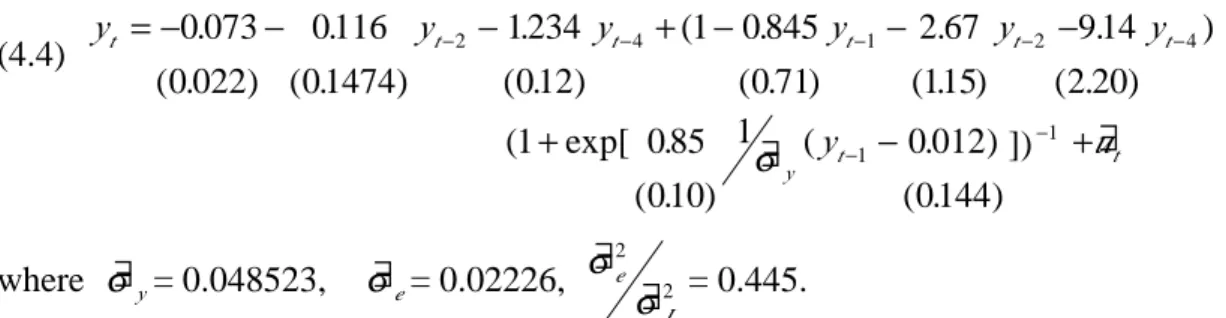
WPI

(4.4) yt = −0 073− yt− − yt− + − yt− − yt− − yt− 0 022 0 116 0 1474 1 234 012 1 0 845 0 71 2 67 115 9 14 2 20 2 4 1 2 4 . ( . ) . ( . ) . ( . ) ( . ( . ) . ( . ) . ( . ) ) ( exp[ . ( . ) ∃ ( . ) ( . ) ]) 1 0 85 0 10 1 _{0 012} 0 144 1 1 + ₋ − − σy t y + ∃u_t where σ∃_y= 0.048523, σ∃_e= 0.02226, σ∃e_σ∃ L 2 2 = 0.445.

The objective function reach its optimum value as 0.0503. The variance ratio is dramatic smaller than the linear AR(4) model. However we do see some distict outier in Figure 2. If we fit the linear AR(4) model again with outliers as dummy variables,

the ratios are not that big, but still smaller. From this we can conclude that LSTAR

model is capable model those exogenous shocks. The dynamics of the model can be deduced from Table 6. The most prominent pair of complex roots in both regime have explosive real roots. It indicates the stationarity of the process if no shocks affect. This also makes the series move between both regime very quickly and oscillate in between. Moreover, the series could diverge from both direction. This will depend on the shock to move it back to both regime. Note the upper regime has a real root with big modulus. It makes the process very explosively. It is possible to lead to the hyper-inflation if the process start growth. Although it is explosive in both regime, the long run behavior of the model could reach a unique stable singular point with value

0.0030. However, the unit root test also indicates no further stationarity in the process. The effect of shocks or what cause such phenomena still needs investigation.

Table 5 contains various diagnostics associated with these models. In general, the ARCH statistics and serial correlation statistics show no sign of significance.

However, the normality test statistics still far from the critical value. However the test statistics are smaller then the linear model. This is a warning there might be some

outliers, the STAR model is not adequate to capture those shocks.

It is not easy to get a decent estimators of linear time series such as STAR model for

the reason that too many possibilities can be encountered and run into troubles. It is also well known that different sets of parameters can give the same functional value in

the linear fit. Furthermore, the estimating procedure to find significant t-statistics of

estimator is troublesome. When a problem occurs, the estimation procedure might

stop, cannot converge, or can not get the final variance-covariance matrix to see the

p-value of the estimated coefficients.

While estimating the STAR model, this practice gives us some ideas how to do a

model with all the possible lags. Second, try bunch of different initial values and find the lowest object function. Third, restrict some parameters to fixed value or find the similar (different sign) value of parameters of the same lags in two different regime. Fourth, exclude those parameters from doing estimation and redo estimation again. Fifth, check the residual from fitted regression. If it is not appropriate, repeat from step three.

Step one coincides with the methodology of “from general to simple” proposed by Hendry (1985). No only the argument of Hendry to find a generally accepted model applies here, we also have the mission to find the lowest value of the objective function. The more lags included in the estimation, the better possibility we can find the minimum value. However, too many lags might lead to the singularity in the Hessian which make it impossible for us to get the variance-covariance matrix.

From step two we can find the lowest possible function value. This step serves as a guide line to find the functional value of the best fit-model. And starting from step three, we begin to reduce the extra parameters to a simple model. By restricting and deleting the redundant parameters, we can get a convergence of the model and have

significant t statistics of the parameters. Step five is just a standard procedure to

search the final model. Note that, when deleting the insignificant variables, we had better do it one by one. Because erase too many lag variables at a time might affect the function values and never get to the optimum. Also in step three, there is no general rule to decide the order of which variable to be deleted first. Extensive experiments are necessary to search for the best model.

5. Conclusion

The result of filter test in Taiwan macroeconomic variables shows most of the real variables do not detect such effect. No asymmetric facial traits in the low level or high level to have the mean reverting. However the price deflators, nominal GNP AND

industrial production in GNP do show the filter. The estimated STAR models for

those linear variables have similar features. Most of the models suggest that the

dynamics of the series during lower regime are different from higher regime. This also symbolize the behavior of recession and expansion. The industrial production of the GNP shows moving from deep recession into higher growth very aggressively, whereas there is nothing in the dynamics of the expansionary regime to suggest a rapid fall into a contraction. Only a sufficiently large negative shock could cause this. The MQM is just the reverse. Though the price deflator from foreign income reveal

very stationary but switching regime. The modeling of WPI is quite different. The characteristic polynomial in both regimes displays at least one complex pair of

explosive roots. This makes it fluctuate widely both upwards and downwards. The dynamic is very strong. Actually, the CPI index has even stronger energy. We exclude this variable to do model because we think it might not be good for the demonstration of smooth transition.

All of the results are, of course, rather rough, because the data used to model is regular and seasonal differnced. We are not comfortable using the seasonal adjusted data for the possibility of information loss. However, we still suffer the over

difference using seasonal difference. Besides, two dominating features during the relatively short observation period are the exogenous shocks associated with the first and second oil cries. The WPI case, notably, the filter is strongly needed. But it might be just to model the response to a single large negative shocks. We can hardly argues that nominal variables in our economy are inherently filter on this basis, but the response to large negative shocks is stronger than that predicted by a linear autoregressive model. More study is needed why real variables do not have the asymmetric effect in the business cycle and the dynamics of price deflators and nominal variables.

The fact that asymmetric behavior in lower regimes and upper regime in most of the

model leads credibility to the LSTAR model. In addition, the ESTAR model seems

appropriate to model our price deflator from foreign income. Even though the STAR

models do not seem to be to model data with too many outliers. The general

conclusion is that in many cases the STAR model family is a suitable tool for

describing the filter found in our macroeconomic series and it can be applied to other economy.

Reference.

Christiano,Lawrence,1988,Why dose invenyory investment fluctuate so much?, Journal of Monetary Economics 21, 247-280.

King, Robert G.,C.I.Plosser and S.T.Robelo,1988a,Production, growth, and business cycles:I. The basic neoclassical model, Journal of Monetary Ecomomics 21,195-232.

King, Robert G.,C.I.Plosser and S.T.Robelo,1988b,Production, growth, and business cycles:II.Newdirections,Journal of MonetaryEconomics21.309-342.

flactuations. Economentrica 50,1345-1370.

Mitchell, Wesley C.,1927, Business cycles: The problem and its setting (Nation Bureau of Economic Research,New York,NY).

Nelson, Charles and Charles Plosser,1982 Trends and random walks in macroeconomic time, series,Journal of Monetary Economics 10, 139-167.

Waston, Mark, 1986, Univariate detrending methods with stochastic trends, Journal of Monetary Economics 18 49-76.

Whittle, Peter, 1963, Predicyion and regulation (Van Nostrand, Princeton, NJ).

Campbell,J.Y. and N.G.Mankiw.1987. Are output fluctuations ttranstory? Quarterly Journal of economics 102 857-80.(a)

Long, J.B.,and C.Plosser.1983.Real businness cycles. Journal of Political Economy 91:39-69.

Shapiro,M.D.1987.Are cyclical fluctuations in productivity due more to supply shocks or demand shocks? American Economic Review Proceedings 77: 118-124.

Sims,C.A.1986.Are Policy models usable for policy analysis? Quarterly Review federal Reserve Bank of Minneapolis (Winter) 2-16.

Lucas,R.E.,1987,Models of businness cycles (Basil Blackwell, Oxford).

Nelson,C.R. and H. Kang,1981, Suprious periodicity in inappropriately detrended time series Econometrica 49, 741-751.

Singletin, K.J., 1988, Econometric issues in the analysis of equilibrium businness cycle models. Journal of Monetary Economics 21, 361-368.

Watson, M.W.,1993, Measures of fit for calibrated models, Journal of Political Economy 101, 1011-1041.

Burns, Arthur M. and Wesley C. Mitchell, Measuring Businness Cycles, New York,N.Y. National Bureau of Economic Research,1946.

Hodrick, Robert J. and Edward Prescott, "Post-war U.S. Business Cycles: An Empirical Investigation," working paper, Carnegie-Mellon,1980.

King, Robert G. and Sergio T. Rebelo, "Low Frequency Filtering and Real Business Cycles," Journal of Economic Dynamics and Control, Vol.17,no.1 (January 1993), 207-231.

King, Robert G. and Charles I. Plosser, "Real Business Cycles and the Test of the Adelmans," Journal of Monetary Economics, forthcoming,1994.

King, Rebert G. and Mark W. Watson, "The Post-War U.S. Phillips Curve: A Revisionist Econometric History," Carnegie Rochester on Public Policy, November 1994.

Prescott, Edward C., "Theory Ahead of Business Cycle Measurement," Carnegie Rochester Conference Series on Public, 25, Fall 1986, 11-66.

Watson, Mark W. "Business Cycle Duration and Postwar Stabilization of the U.S.Economy," American Economic Review, vol.84,no.1 (March 1994),24-46. Lucas,R.E.Jr.(1972), 'Expectations and the Neutrality of Money', Journal of Economic

Theory, April.

Lucas, R.E.Jr.(1973), 'Some Interational Evidence on Output-Inflation Tradeoffs', American Economic Review, June.

Lucas, R.E.Jr.(1988),'on the Meshanics of Economic Development', Journal of Monetary Economics, July.

Prescott, E.C. (1986), 'Theory Ahead of Business Cycle Measurement', Federal Reserve Bank of Minneapolis Quarterly Review, Fall.

Sargent,T.J. and Wallace, N.(1975), 'Rational Expectations, the Optimal Monetary Instrument and the Optimal Money Supply Rule', Lournal of Political Economy,

April.

Sargent,T.J. and Wallace, N.(1976), 'Rational Expectations and the Theory of Economic Policy, April.

Sims,C.A.(1980), 'Comparisons of Interwar and Postwar Business Cycles: Monetarism Reconsidered', American Economic Review, May.

Sims,C.A.(1983), 'Is There a Monetary Business Cycle?', American Economic Review, May.

Solow,R.M.(1956), 'A Contribution to the Theory of Economic Growth', Quarterly Journal of Economics, February.

Slolw,R.M.(1957), 'Technical Change and the Aggregate Production Function', Review of Economics and Statistics, August.

Solow,R.M.(1980), 'On Theories of Unemployment', American Economic Review, March.

Solow,R.M.(1990), The Labour Market as a Social Institution, Oxford: Basil Blackwell.

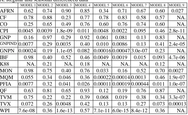
Table 1. Filter test of the two transformed data set: regular differenced seasonal adjusted data, regular and seasonal difference data.

A. Regular and seasonal differenced data

MODEL 1 MODEL 2 MODEL 3 MODEL 4 MODEL 5 MODEL 6 MODEL 7 MODEL 8 MODEL 9

AFRN 0.62 0.74 0.90 0.85 0.34 0.71 0.67 0.60 0.027

CF 0.78 0.88 0.23 0.77 0.78 0.83 0.58 0.57 NA.

CO 0.25 0.65 0.49 0.76 0.60 0.76 0.74 0.60 NA.

CPI 0.0045 0.0039 1.8e-09 0.011 0.0048 0.0022 0.095 0.46 2.8e-11

GNP 0.16 0.97 0.29 0.92 0.061 0.081 0.13 0.83 NA.

GNPIND _{0.0077 0.29 0.0035 0.40 0.010 0.0086 0.13 0.41 2.4e-05}

GNPN 0.00024 0.19 1.1e-05 0.082 0.00016 0.00047 3.0e-07 0.23 NA.

IBF 0.98 0.40 0.52 0.46 0.0049 0.0019 0.015 0.093 4.7e-06

K88 NA. 0.21 NA. 0.18 NA. NA. NA. 0.12 NA.

MON 0.98 0.75 0.40 0.76 0.033 0.16 0.52 0.70 0.0027 MQM 0.055 0.34 0.046 0.36 0.00022 0.00014 0.0013 0.46 1.9e-07 PFIA 0.0077 0.32 0.041 0.026 0.00011 0.00019 0.00044 0.011 1.0e-07 QF 0.63 0.81 0.65 0.93 0.12 0.19 0.76 0.87 NA. TVM 0.75 0.22 0.22 0.39 0.068 0.019 0.38 0.34 3.3e-07 TVX 0.072 0.26 0.0048 0.42 0.13 0.13 0.27 0.073 0.00013

WPI 7.6e-08 0.36 1.6e-13 0.57 7.1e-11 6.0e-15 8.4e-12 0.36 NA.

B. Regular differenced seasonal adjusted data

MODEL 1 MODEL 2 MODEL 3 MODEL 4 MODEL 5 MODEL 6 MODEL 7 MODEL 8 MODEL 9

AFRN 0.24 0.35 0.080 0.45 0.15 0.11 0.090 0.16 0.0012

CF 0.38 0.36 0.10 0.56 0.42 0.76 0.28 0.37 NA.

CO 0.41 0.53 0.80 0.49 0.53 0.59 0.64 0.NA NA.

CPI 2.0e-07 0.0060 3.2e-11 0.010 5.8e-07 1.9e-10 5.7e-12 0.076 2.8e-12

GNP 0.057 0.023 0.0017 0.042 0.11 0.0024 0.39 0.015 NA.

GNPIND _{0.063 0.23 0.027 0.31 0.0068 0.025 0.037 0.14 9.8e-06}

GNPN 0.50 0.66 0.0012 0.29 0.023 0.016 0.00022 0.15 NA.

IBF 0.021 0.57 0.17 0.14 0.0063 0.041 0.00027 0.24 NA.

K88 0.97 0.90 NA. 0.75 NA. NA. NA. 0.55 NA.

MON 0.0061 0.35 0.011 0.33 0.0055 0.0015 0.13 0.19 4.2e-06

MQM 0.30 0.0011 0.00075 8.5e-05 0.43 6.8e-05 0.00025 0.72 6.8e-08

PFIA 0.0019 0.0045 0.016 0.0051 0.010 0.023 0.014 0.0026 NA.

QF 0.44 0.36 0.31 0.56 0.57 0.42 0.64 0.62 NA.

TVM 0.67 0.66 0.11 0.42 0.15 0.14 0.15 NA 4.2e-05

TVX 0.98 0.015 0.042 0.040 0.66 0.065 0.73 0.024 5.1e-05