國 立 交 通 大 學
機 械 工 程 學 系
碩 士 論 文
利用流體體積法之雙流體計算
Calculation of Two-Fluids Flow
Using Volume-of-Fluid Method
研 究 生:鄭 東 庭
指 導 教 授:崔 燕 勇 博士
利用流體體積法之雙流體計算
Calculation of Two-Fluids Flow Using Volume-of-Fluid Method
研 究 生:鄭 東 庭 Student:Tong-Ting Cheng
指導教授:崔 燕 勇 Advisor:Yeng-Yung Tsui
國立交通大學
機械工程研究所
碩士論文
A Thesis
Submitted to Institute of Mechanical Engineering
Collage of Engineering
National Chiao Tung University
In Partial Fulfillment of the Requirements
For the degree of
Master of Science
In
Mechanical Engineering
July 2007
Calculation of Two-Fluids Flow Using Volume-of-Fluid Method
Student:Tong-Ting
Cheng
Advisor:Prof. Yeng-Yung Tsui
Institute of Mechanical Engineering National Chiao Tung University
ABSTRACT
In two fluid flow investigation, the simulation of flows with free surfaces is difficult because neither the shape nor the position of the interface can be identifies in advance between two immiscible fluids. The aim of this study is to develop a scheme, which ensures the preservation of the sharpness and the shape of the interface while retaining boundedness of the field, by volume tracking method and blending strategy without explicit interface reconstruction. The motion of the interface is tracked by the solution of a transport equation for a phase-indicator field. Furthermore, this scheme is formed and compared with the well-known HRIC, CICSAM and STACS schemes. Some favorable cases are simulated and comparisons are made in the literature.
利用流體體積法之雙流體計算
研究生 鄭東庭 指導教授 崔燕勇 博士 國立交通大學機械工程學系 摘要 在雙流體之研究中,在模擬流場時兩不互溶流體之自由液面的位置與形狀難以去確 認。本研究之目的為以流體體積法及混合策略建立一模擬架構,且不需經由以重建自由 液面之方式,以期能保持自由液面形狀之明確性並符合流場中之邊界性。而流場中自由 液面之運動乃經由求解一傳輸方程式所得。更進一步地,在模擬架構建立之後,將與前 人所發展之方法比較,如 Muzaferija 提出之 HRIC 法、Ubbink 提出之 CICSAM 法、以及 Dariwish 所提出之 STACS 法。另外,此架構將應用在一些案例,並與實驗成果及前人數 值模擬之結果作比較。Acknowledgments
I would like to express my deepest gratitude to my supervisor, Prof. Yeng-Youg Tsui, for his constructive criticism, guidance provided throughout my research, patience and continuous support. I've learned the research methods and attitudes from his instruction during the two-year courses.
I would like to thank all the members and previous members of CFD Laboratory.
Thanks to the senior students, Yu-Chang Hu and Tian-Cherng Wu for their suggestion and guidance. They helped me solve many problems and introduced me good research directions. Thanks to Eatrol Lu for his great help and companion. We built a good friendship during the two years. It’s definitely too hard to forget the time we work together, especially the month before oral presentation.
I would like to thank all the members of Ballroom Dance Club in our school. Dancing is the most important and stress-releasing recreation in my leisure time. Y-Ching Cheng, Yun-Yun Song, Deniel Wu and Jing-Wen Wu are all famous dancers. Thanks to them for teaching me to dance. Thanks to Gloria Lin and Jamin Chang. We gave good performances together.
Finally, I would like to thank my family for their support and encouragement. Thanks to my uncle Wen-Fong Cheng and Sunny Gao. I really appreciate that they taught me the style of handling problem and getting along with people. I am also so appreciated my dad Wen-Yao Cheng, my mom Yue-Feng Chen, my brother Andy Cheng and my girlfriend Karen Liu. They are the most important spiritual support in my whole life.
Content
ABSTRACT ... i
Content ... iv
List of Figures ... vi
Nomenclature... x
Abbreviation ... xii
Chapter 1 Introduction... 1
1.1 Background ...1 1.2 Related Studies...11.3 Present study of this thesis...7
Chapter 2 Mathematical Model... 9
2.1 Introduction ...9
2.2 General transport equation ...9
2.3 Governing equations ...10
Mass conservation ...10
2.4 Surface tension...12
2.5 Boundary Conditions ...14
2.6 Closure...14
Chapter 3 Numerical Method for the VOF Equation... 15
3.1 Introduction ...15
3.2 The approximation for the face value of α ...15
3.3 Linear difference schemes...17
3.4 Non-linear difference schemes...19
3.5 The normalized variables for unstructured-grids ...24
3.6 Discretization of the indicator equation ...25
3.7 Blending strategy ...27
4.1 Introduction ...32
4.2 Discretization ...32
4.3 Pressure-velocity coupling with PISO ...35
4.4 Solution procedure for the two-fluid system ...40
Chapter 5 Results and Discussion... 41
5.1 Introduction ...41
5.2 The VOF schemes test in an oblique velocity field...41
5.3 Surface tension...59 5.4 Drop splash...62 5.5 Bubble...65 5.6 Sloshing...68 5.7 Rayleigh-Taylor instability ...74 5.8 Column collapse...93 5.9 Hydraulic bore ... 113
Chapter 6 Conclusion and Future Work ... 120
List of Figures
FIGURE 1.1(A) SURFACE METHODS (B) VOLUME METHODS... 2
FIGURE 1.2SCHEMATIC REPRESENTATION OF MARKER AND CELL MESH LAYOUT... 3
FIGURE 1.3INTERFACE RECONSTRUCTIONS OF (A) ACTUAL FLUID CONFIGURATION,(B)SLIC IN X-DIRECTION,(C) SLIC IN Y-DIRECTION (D)YOUNGS’VOF... 4
FIGURE 2.1GENERAL FORM OF THE CONSERVATION LAW... 10
FIGURE 2.2FLUIDS ARE MARKED WITH INDICATOR FUNCTION... 11
FIGURE 2.3CONTINUITY OF THE VELOCITY FIELD AND DISCONTINUITY OF THE MOMENTUM... 12
FIGURE 2.4FLUID ARRANGEMENT AND THE SIGN OF THE CURVATURE... 13
FIGURE 3.1 THE RELATIONSHIP OF A CONTROL VOLUME AND ITS NEIGHBOR CELLS... 15
FIGURE 3.2NORMALIZED VARIABLE DIAGRAM (NVD). ... 17
FIGURE 3.3RELATIONSHIP BETWEEN γ AND rFOR LINEAR DIFFERENCE SCHEMES. ... 19
FIGURE 3.4TVDCONSTRAINTS IN (A)NVD AND (B)TVD DIAGRAM... 20
FIGURE 3.5SMART... 22 FIGURE 3.6MUSCL... 22 FIGURE 3.7SUPERBEE ... 22 FIGURE 3.8STOIC... 23 FIGURE 3.9OSHER ... 23 FIGURE 3.10BDS... 23 FIGURE 3.11VAN LEER... 24 FIGURE 3.12CHARM... 24
FIGURE 3.13.THE PREDICTION OF UPWIND VALUE FOR AN ARBITRARY CELL ARRANGEMENT... 25
FIGURE 3.14(A) THE INTERFACE IS PARALLEL TO THE FLOW DIRECTION AND THE COMPRESSIVE SCHEME WILL BE USED (B) THE INTERFACE IS PERPENDICULAR TO THE FLOW DIRECTION AND HIGH RESOLUTION SCHEMES ARE APPROPRIATE. ... 27
FIGURE 3.15THE NVD OF (A)HYPER-C AND (B)UQ AT Cof EQUAL 0.5 ... 29
FIGURE 3.16A,3.16B AND 3.16C SHOW THE RELATIONSHIP BETWEEN TWO SCHEMES FOR HRIC,CICSAM AND STACS.THE X-AXIS STAND FOR θf AND Y-AXIS MEANS THE VALUE OF f
( )
θf ... 31FIGURE 4.1ILLUSTRATION OF THE PRIMARY CELL P AND THE NEIGHBOR CELL NB WITH A CONSIDER FACE F... 33
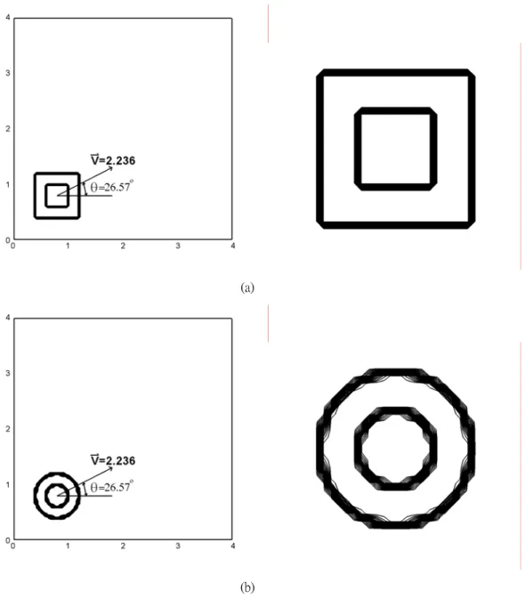
FIGURE 5.1THE FLOW FIELD DOMAIN AND INITIAL CONDITION OF (A) HOLLOW SQUARE,(B) HOLLOW CIRCLE... 43
FIGURE 5.3(A)COMPARISON OF DIFFERENT SCHEMES WITH GRIDS 100*100 AND COURANT NUMBER=0.75 (ΔT=0.01)... 45
FIGURE 5.3(B)COMPARISON OF DIFFERENT SCHEMES WITH GRIDS 100*100 AND COURANT NUMBER=0.50 (ΔT=0.00667)... 46
FIGURE 5.3(C)COMPARISON OF DIFFERENT SCHEMES WITH GRIDS 100*100 AND COURANT NUMBER=0.25 (ΔT=0.00333)... 47
FIGURE 5.4(A)COMPARISON OF DIFFERENT SCHEMES WITH GRIDS 100*100 AND COURANT NUMBER=0.75 (ΔT=0.01)... 48
(ΔT=0.00667)... 49
FIGURE 5.4(C)COMPARISON OF DIFFERENT SCHEMES WITH GRIDS 100*100 AND COURANT NUMBER=0.25 (ΔT=0.00333)... 50
FIGURE 5.5COMPARISON OF HRIC,CICSAM AND STACS WITH GRIDS 100*100... 53
FIGURE 5.6(CONTINUE)COMPARISON OF DIFFERENT COMPOSITE SCHEMES WITH GRIDS:100*100... 54
FIGURE 5.6COMPARISON OF DIFFERENT COMPOSITE SCHEMES WITH GRIDS:100*100 ... 55
FIGURE 5.7COMPARISON OF HRIC,CICSAM AND STACS WITH GRIDS:100*100... 56
FIGURE 5.8 COMPARISON OF DIFFERENT COMPOSITE SCHEMES WITH GRIDS:100*100... 57
FIGURE 5.8COMPARISON OF DIFFERENT COMPOSITE SCHEMES WITH GRIDS:100*100. ... 58
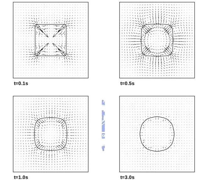
FIGURE 5.9TIME EVOLUTION OF THE SHAPE CHANGES OF A SQUARE SUBJECTED TO SURFACE TENSION FORCES. ... 60
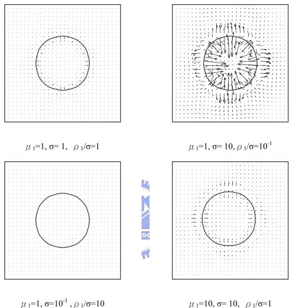
FIGURE 5.10PARASITE CURRENTS FOR DIFFERENT VISCOSITY OF FLUID 1 AND SURFACE TENSION COEFFICIENT. ... 61
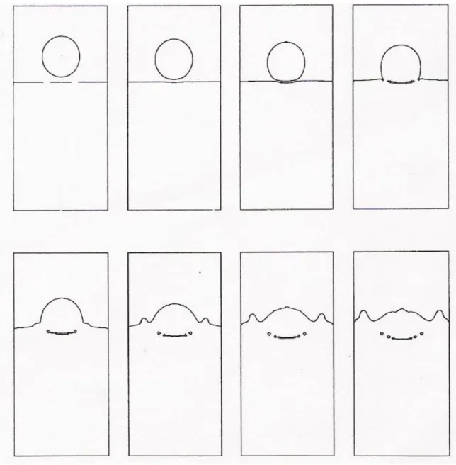
FIGURE 5.11 THE WATER DROPLET FALLING AIR ONTO SURFACE AT TIMES T=0.0S,0.00677S,0.00980S,0.01220S, 0.01485S,0.01781S,0.01995S,0.02146S.(BY PUCKETT ET AL.[38])... 63
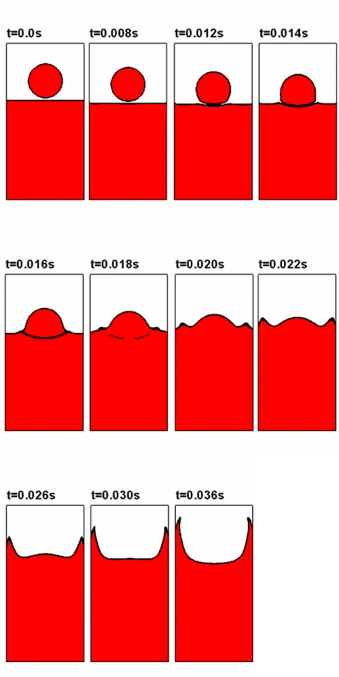
FIGURE 5.12WATER DROPLET FALLING THROUGH AIR ONTO WATER SURFACE.THE TIME STEP SIZE IS 0.00005 AND COMPUTATIONAL DOMAIN IS 0.007*0.014(64*128).THE MAXIMUM COURANT NUMBER DURING COMPUTATION IS 0.24 ... 64
FIGURE 5.13TIME EVOLUTION OF AN AIR BUBBLE RISING THROUGH WATER WITHOUT SURFACE TENSION. ... 66
FIGURE 5.14TIME EVOLUTION OF AN AIR BUBBLE RISING THROUGH WATER WITH SURFACE TENSION. ... 67
FIGURE 5.15THE PHYSICAL MODEL OF SLOSING... 68
FIGURE 5.16TIME EVOLUTION OF THE WAVE POSITION AND VELOCITY VECTORS FOR THE FIRST PERIOD OF SLOSHING OF AN INVISICD FLOW FIELD WHICH INFLUENCED BY GRAVITY.THE COMPUTATIONAL GRIDS ARE 160*104.THE MAXIMUM COURANT NUMBER DURING THE COMPUTATION:0.03... 72
FIGURE 5.17POSITION OF THE INTERFACE AT THE LEFT BOUNDARY AGAINST THE TIME (INVISCID FLOW). ... 73
FIGURE 5.18POSITION OF THE INTERFACE AT THE LEFT BOUNDARY AGAINST THE TIME (VISCOUS FLOW).THE AMPLITUDE OF SLOSHING WILL DECREASE WITH THE TIME GOES BY... 73
FIGURE 5.19(A)THE PHYSICAL MODEL OF RAYLEIGH-TAYLOR INSTABILITY.(B)THE ARRANGEMENT OF UNIFORM GRIDS (64*192).(C)THE ARRANGEMENT OF NON-UNIFORM GRIDS (80*284) ... 74
FIGURE 5.20(A)THE FIRST KIND OF INITIAL CONDITION.(B)THE SECOND KIND OF INITIAL CONDITION (C)THE THIRD KIND OF INITIAL CONDITION. ... 76
FIGURE 5.21THE NUMERICAL RESULTS OF RAYLEIGH-TAYLOR INSTABILITY ADOPTING 1ST KIND OF INITIAL CONDITION WITH UNIFORM GRIDS 64*192. ... 77
FIGURE 5.22THE NUMERICAL RESULTS OF RAYLEIGH-TAYLOR INSTABILITY ADOPTING 1ST KIND OF INITIAL CONDITION WITH NON-UNIFORM GRIDS 80*284... 78
FIGURE 5.23THE NUMERICAL RESULTS OF RAYLEIGH-TAYLOR INSTABILITY ADOPTING 2ND KIND OF INITIAL CONDITION WITH UNIFORM GRIDS 64*192. ... 79
FIGURE 5.24THE NUMERICAL RESULTS OF RAYLEIGH-TAYLOR INSTABILITY ADOPTING 2ND KIND OF INITIAL CONDITION WITH NON-UNIFORM GRIDS 80*284... 80
FIGURE 5.25THE NUMERICAL RESULTS OF RAYLEIGH-TAYLOR INSTABILITY ADOPT 3RD INITIAL CONDITION WITH UNIFORM GRIDS 64*192... 81
FIGURE 5.26THE NUMERICAL RESULTS OF RAYLEIGH-TAYLOR INSTABILITY ADOPTING 3RD KIND OF INITIAL CONDITION WITH NON-UNIFORM GRIDS 80*284... 82
CONDITION WITH UNIFORM GRIDS 64*192. ... 83
FIGURE 5.28THE NUMERICAL RESULTS OF RAYLEIGH-TAYLOR INSTABILITY ADOPTING 4TH KIND OF INITIAL
CONDITION WITH NON-UNIFORM GRIDS 80*284... 84 FIGURE 5.29THE NUMERICAL RESULTS OF RAYLEIGH-TAYLOR INSTABILITY ADOPTING 5TH KIND OF INITIAL
CONDITION WITH UNIFORM GRIDS 64*192. ... 85 FIGURE 5.30THE NUMERICAL RESULTS OF RAYLEIGH-TAYLOR INSTABILITY ADOPTING 5TH KIND OF INITIAL
CONDITION WITH NON-UNIFORM GRIDS 80*284... 86 FIGURE 5.31THE NUMERICAL RESULTS OF RAYLEIGH-TAYLOR INSTABILITY ADOPTING 1ST KIND OF INITIAL
CONDITION WITH NON-UNIFORM GRIDS 64*192 AND SLIP BOUNDARY CONDITION. ... 88 FIGURE 5.32THE NUMERICAL RESULTS OF RAYLEIGH-TAYLOR INSTABILITY ADOPTING 2ND KIND OF INITIAL
CONDITION WITH NON-UNIFORM GRIDS 64*192 AND SLIP BOUNDARY CONDITION. ... 89 FIGURE 5.33THE NUMERICAL RESULTS OF RAYLEIGH-TAYLOR INSTABILITY ADOPTING 3RD KIND OF INITIAL
CONDITION WITH NON-UNIFORM GRIDS 64*192 AND SLIP BOUNDARY CONDITION. ... 90 FIGURE 5.34THE NUMERICAL RESULTS OF RAYLEIGH-TAYLOR INSTABILITY ADOPTING 4TH KIND OF INITIAL
CONDITION WITH NON-UNIFORM GRIDS 64*192 AND SLIP BOUNDARY CONDITION. ... 91
FIGURE 5.35THE NUMERICAL RESULTS OF RAYLEIGH-TAYLOR INSTABILITY ADOPTING 5TH KIND OF INITIAL
CONDITION WITH NON-UNIFORM GRIDS 64*192 AND SLIP BOUNDARY CONDITION. ... 92
FIGURE 5.36EXPERIMENTAL RESULTS OF A COLLAPSING WATER COLUMN BY KOSHIZUKA [40]. ... 95
FIGURE 5.37THE NUMERICAL RESULTS OF COLUMN COLLAPSE WHICH THE TIME STEP SIZE IS 0.00025S AND THE SPATIAL SIZE IS 4.86E-3M (GRIDS:120*70).THE MAXIMUM COURANT NUMBER DURING THE COMPUTATION IS
0.699. ... 96 FIGURE 5.38THE NUMERICAL RESULTS OF COLUMN COLLAPSE WHICH THE TIME STEP SIZE IS 0.001S AND THE
SPATIAL SIZE IS 0.0121M (GRIDS:48*28).THE MAXIMUM COURANT NUMBER DURING THE COMPUTATION IS
0.621. ... 97 FIGURE 5.39THE NUMERICAL RESULTS OF COLUMN COLLAPSE WHICH THE TIME STEP SIZE IS 0.000125S AND THE
SPATIAL SIZE IS 2.43E-03M (GRIDS:240*140).THE MAXIMUM COURANT NUMBER DURING THE COMPUTATION IS 0.563... 98
FIGURE 5.40THE NUMERICAL RESULTS OF COLUMN COLLAPSE WHICH THE TIME STEP SIZE IS 0.00025S AND THE SPATIAL SIZE IS 4.86E-03M (GRIDS:120*165).THE MAXIMUM COURANT NUMBER DURING THE COMPUTATION IS 0.615... 100
FIGURE 5.41THE NUMERICAL RESULTS OF COLUMN COLLAPSE WITH SURFACE TENSION WHICH THE TIME STEP SIZE
IS 0.00025S AND THE SPATIAL SIZE IS 4.86E-3M (GRIDS:120*70).THE MAXIMUM COURANT NUMBER DURING THE COMPUTATION IS 0.699. ... 101
FIGURE 5.42THE NUMERICAL RESULTS OF COLUMN COLLAPSE WITH SURFACE TENSION WHICH THE TIME STEP SIZE
IS 0.001S AND THE SPATIAL SIZE IS 0.0121M (GRIDS:48*28).THE MAXIMUM COURANT NUMBER DURING THE COMPUTATION IS 0.611... 102
FIGURE 5.43THE NUMERICAL RESULTS OF COLUMN COLLAPSE WITH SURFACE TENSION WHICH THE TIME STEP SIZE
IS 0.000125S AND THE SPATIAL SIZE IS 2.43E-03M (GRIDS:240*140).THE MAXIMUM COURANT NUMBER DURING THE COMPUTATION IS 0.485. ... 103
FIGURE 5.44THE NUMERICAL RESULTS OF COLUMN COLLAPSE WITH SURFACE TENSION WHICH THE TIME STEP SIZE
FIGURE 5.45THE POSITION OF THE LEADING EDGE VERSUS TIME. ... 106
FIGURE 5.46THE HEIGHT OF THE COLLAPSING WATER COLUMN VERSUS TIME... 106
FIGURE 5.47EXPERIMENTAL RESULTS OF A COLLAPSING WATER COLUMN HITTING AN OBSTACLE (KOSHIZUKA [40]) ... 108
FIGURE 5.48THE NUMERICAL RESULTS OF COLUMN COLLAPSE WITH OBSTACLE WITHOUT SURFACE TENSION.THE UPPER BOUNDARY AT THE COMPUTATIONAL DOMAIN IS WALL. ... 109
FIGURE 5.49THE NUMERICAL RESULTS OF COLUMN COLLAPSE WITH OBSTACLE WITHOUT SURFACE TENSION.THE UPPER BOUNDARY AT THE COMPUTATIONAL DOMAIN IS OPEN BOUNDARY WHICH PRESSURE IS FIXED. ... 110
FIGURE 5.50THE NUMERICAL RESULTS OF COLUMN COLLAPSE WITH OBSTACLE WITH SURFACE TENSION.THE UPPER BOUNDARY AT THE COMPUTATIONAL DOMAIN IS WALL. ... 111
FIGURE 5.52THE PHYSICAL MODEL OF HYDRAULIC BORE... 113
FIGURE 5.53SCHEMATIC REPRESENTATION OF GRID CONFIGURATION FOR THE BORE... 113
FIGURE 5.54VELOCITY VECTORS AND FLUID CONFIGURATION FOR THE BORE CALCULATED WITH G=1.0 AT TIMES 3.5S,4.9S,8.0S,10.0S AND 12.0S. ... 115
FIGURE 5.55VELOCITY VECTORS AND FLUID CONFIGURATION WITH VELOCITY U=1.0 AT INLET... 117
FIGURE 5.56VELOCITY VECTORS AND FLUID CONFIGURATION WITH VELOCITY U=2.0 AT INLET... 118
Nomenclature
A Coefficient of algebraic equation
Co Courant number
C
F Boundary flux due to convection
D
F Boundary flux due to diffusion
f Face, point in the centre of the face
P
f Weighting factor
σ
f Surface tension force
g Gravitational acceleration
f
m& Mass flow rate cross face
P Pressure
S Source term in discretized momentum equation
α
S Source term in discretized the indicator equation
t Time
f
w Weighting factor
y
x, Components of Cartesian coordinate
Pnb
δr Vector pointing from center of primary cell to the center of neighbor one
Γ Diffusivity φ Property ∀ Δ Volume ) (r
γ Flux limiter equation
α Volume fraction
σ Surface tension coefficient
ρ Fluid density
μ Viscosity coefficient
Δ Difference operator
∇ Gradient
f
θ Angle between the normal to interface and orthogonal component of the face area vector
n New time level
Abbreviation
BD Bounded Downwind Scheme
CBC Convective Boundedness Criterion
CFD Computational Fluid Dynamics
CDS Central Difference Scheme
CICSAM Compressive Interface Capturing Scheme for Arbitrary Meshes CN Crank-Nicolson
CUBISTA Convergent and Universally Bounded Interpolation Scheme CUS Cubic upwind difference scheme
CV Control Volume
DDS Downwind Difference Scheme
HRS High Resolution Scheme
LUS Linear Upwind Scheme
MAC Marker and cell
MINMOD Minimum Modulus
MUSCL Monotonic Upwind Scheme for Conservation Law
NVD Normalized Variable Diagram
PISO Pressure Implicit with Splitting of Operator
QUICK Quadratic Upwind Interpolation for Convection Kinematics SLIC Simple Line Interface Calculation
SMART Sharp and Monotonic Algorithm for Realistic Transport STOIC Second- and Third-Order Interpolation for Convection
TVD Total Variation Diminishing
UDS Upwind Difference Scheme
Chapter 1 Introduction
1.1 Background
The simulation of two immiscible fluids separated by a well-defined interface has many applications. One area is the biochemical science engineering where it is used to simulate biochemical material or fluids such as blood being transported through the capillary tubing and channels in the vascular system or in Micro Electro Mechanical Systems (MEMS) devices. In the environmental engineering, free surface flows are used in the simulation of motion of water in the marine environment, volcanic flows and plumes, and Dam and dyke breaks. On the other hand, to shorten the design of the digital inkjet printing technology, numerical simulations seem to be the require tool. Yeh [1] used a simple but versatile finite element method for the simulation of piezoelectric inkjet. Liou et al. [2] simulated the SEAjet (Static-Electricity Actuator inkJET) [3] by finite volume method. This technology has significant influences on other relevant applications, such as IC package process and LED screens, etc.
1.2 Related Studies
The computation of flows with free surfaces is difficult in the prediction of the shape and the position of the interface between two immiscible fluids. Hirt and Nichols [4] illustrated that three types of problems arise in the numerical treatment of free surfaces: (1) their discrete representation, (2) their evolution in time, and (3) the manner in which boundary conditions are imposed. Therefore, it is important to develop robust methods to capture interfaces. Such methods in finite volume approach can be classified into two typical categories: surface methods and volume methods [5]. In the following, these methods are briefly reviewd.
(a) (b)
Figure 1.1 (a) surface methods (b) volume methods
Surface methods, which are called interface-tracking method, mark and track the interface with calculation only on one phase based on the satisfaction of two conditions. First, the free surface is a sharp interface between the two fluids and there is no flow across the interface. Second, forces acting on the interface are in equilibrium. These methods only compute the liquid flow and the computational grids vary with the shape and position of the free surface. The differences between surface methods and volume methods can be shown as Figure 1.1. By surface methods the grid fits the interface and moves with it. The free surface is treated as a boundary of the computation domain. The advantage of this approach is that the interface remains sharp as it is across the mesh and the surface tension force is included in the subsequent implement without be coped specially. On the other hand, interface-tracking or moving meshes methods can not be used if the interface changes significantly. There are several interface-tracking (surface) methods which mark and track the interface explicitly, (i) with a set of marker particles or line segments on interface [6], or (ii) height functions [7], (iii) level set method [8], and (iv) surface fitted methods. [5]
In volume methods, the different fluids are marked either by massless particles or by an indicator function which may turn to be volume fraction. The advantage of these methods is their ability to cope with the arbitrary shaped interface and large deformation. One of the main difficulties associated with these methods is the advection of the interface without
The earliest numerical technique designed for simulating free surface flows was the well-known marker and cell (MAC) method [9] .The MAC method use massless marker particles which spread over the volume occupied by a fluid with a free surface (see Figure 1.2). A cell with no marker particles is considered to be empty. This method can treat complex phenomena like wave breaking. Although the MAC method can tackle arbitrary unstructured grids, there two problems arise in further simulation. First, the disadvantage of this method is that the computer storage will increase significantly and time consuming is largely increased in three-dimension of calculations. The other is that it is also difficult to obtain quantitative information on interface orientation. However, some improved versions have been presented, for example by Chen et al. [10]
Figure 1.2 Schematic representation of marker and cell mesh layout.
Several volume tracking methods for finite volume and arbitrary meshes have been developed with the aim of maintaining sharp interfaces. The better known methods are Simple Line Interface Calculation (SLIC) method [11], the volume-of-fluid (VOF) method [5] and the method of Youngs[12].
(a) Actual fluid configuration (b) SLIC (x-direction)
(c) SLIC (y-direction) (d) Youngs’ VOF
Figure 1.3 Interface reconstructions of (a) actual fluid configuration, (b) SLIC in x-direction, (c) SLIC in y-direction (d) Youngs’ VOF.
The SLIC method [11] approximates interfaces as piecewise constant, where interfaces within each cell are reconstructed using straight lines parallel to one of the coordinate directions. It is a direction-split algorithm and during each direction sweep, only cell neighbors in the sweep direction are used to determine the interface reconstruction. (Figure 1.3(b) and 1.3(c)). An extensive review of this type of methods can be found in [13].
Youngs’ VOF (Y-VOF) [12] method uses a more accurate interface reconstruction than the SLIC method. Youngs give a useful refinement to the SLIC method with the use of oblique lines to approximate the interface in the cell (Figure 1.3(d)). Unlike the SLIC method, the neighbor cells are used to approximate the slope of the interface in Youngs’ VOF. The SLIC method and Youngs’ VOF can be classified as line technique and these methods use structured grids and are therefore restricted to such mesh topologies.
volume tracking methods in the simulation and prediction of two-fluid system with interfaces where density and viscosity change abruptly. The VOF method became popular in the 80s though the development of this method occurred earlier [9,14]. Its appealing feature is its volume fluxes can be formulated algebraically without reconstructing the interface. The interfaces are represented by the value of the VOF function which is a volume fraction of one of the fluids. Another benefit of using volume fractions is that only a scalar convection equation, which is called indicator equation, need to be solved to propagate the volume fractions through the computational domain. In the calculation of convective fluxes, two of the main errors in numerical modeling of convection-diffusion transport problems are numerical diffusion and numerical dispersion. Numerical diffusion causes smearing of predicted profile, and numerical dispersion results in non-physical phenomenon such as oscillation or over/under shoots produced in the solution.
Because the first-order upwind scheme is too diffusive, differencing schemes of order higher than unity are therefore required. Second-order accuracy can be achieved by linear interpolation from two upwind values, yield so-called linear upwind schemes (LUDS) of Shyy et al. [15]. Third-order accuracy is achieved by a quadratic line through those two upwind values and one downwind, the QUICK scheme of Leonard [16]. These schemes get more accurate results than first-order upwind, but they are not bounded which may give rise to oscillations in the region where there are strong gradients of the variable being solved. There are two major categories to handle these numerical dispersion problems, known as flux-blending and composite flux-limiter methods. The flux-blending method can be divided into two classes. The first class is added an anti-diffusion flux to a first order upwind scheme, for example, Zalesak presented the flux corrected transport (FCT) method [17]. In the second class, a smoothing diffusive flux is introduced into an unbounded higher order schemes. In generally speaking, due to the nature of flux-blending method, the numerical dispersion can be reduced but it will be very expansive computationally and the optimal blending factor can not be obtained easily.
[18] to enhance the accuracy of simulation. The first order upwind is diffusive and stable. The first order downwind is unstable, but has the advantage of maintain sharp interface. If a suitable combination of upwind and downwind fluxes can be formulated, a volume tracking algorithm can be designed. Hence, this method combines the low order scheme and higher order scheme. Although the FCT-VOF method is non-diffusive in nature, but create unphysical flotsam and jetsam.
As everyone knows, only the first order upwind difference scheme satisfies the sufficient condition of the Convective Boundedness Criteria (CBC) [23]. In order to fit in with the CBC, a higher order difference scheme has to be a non-linear combined framework. In the composite flux-limiter method, the numerical flux at a consider face is adjusted by the flux-limiter function. Normalized Variable (NV) and Normalized Variable Diagram (NVD) which presented by Leonard [19] are important implements for the composite flux-limiter method and simplify the connection between high accuracy and bounedness in high resolution schemes (HRs) [20].
At first, the flux limiter function is presented by Van Leer [21]. Sweby [22] developed the Total Variation Diminishing (TVD) approach for high resolution schemes. Flux limiter functions were introduced to guarantee that values of a conserved property remain within the bounds. The accurate simulation of convection continues to attract many workers due to the many challenges it still offers. The difficulty in devising an effective scheme lies in the conflicting requirements of accuracy, stability and boundedness. There are many high resolution schemes developed in these years, such as SMART of Gaskell and Lau [23], GAMMA of Jasak [24], SUPERBEE of Roe [25], STOIC of Darwish [26], MUSCL and Van Leer of Van Leer [27]
Numerical diffusion, a significant source of error in numerical solution of conservation equations, can be separated into two components, namely cross-stream and stream-wise numerical diffusions. The former, the cross-stream numerical diffusion, occurs in a multi-dimensional flow when the flow direction is perpendicular to the grid lines. The latter,
lines.
In addressing aforementioned issue, many researchers try to improve the accuracy by reducing streamwise and cross-stream numerical diffusion. Hence, the blending strategy that depends on the angle between the flow direction and the grid lines was developed. The best approach is to have a continuous switching function whereby the values of compressive and high resolution schemes are blended together with a blending factor. This general approach has been followed in the derivation of composite schemes and is utilized in the HRIC of Muzaferija [28], STACS of Darwish [29] and CICSAM of Ubbink [30].
1.3 Present study of this thesis
The aim of this study is to develop a robust scheme which is accurate, stable and easy to be implemented on arbitrary unstructured grids. The two-fluid system will be modeled by the volume tracking method. This research is considered to be two-dimensional under unsteady and incompressible conditions with body forces of gravity and surface tension.
In Chapter 2, the conception of conservation laws which are used to construct the governing equations is introduced. The governing equations in two-fluid system are given and the mathematical model of the surface tension term in the momentum equation will be made. Chapter 3 introduces the numerical method and discretization of the VOF equation. The blending strategy was developed and used in constructing volume tracking approach is described. This is followed by a discussion of the general strategy used for switching between compressive and high resolution schemes.
In Chapter 4, a conservative finite volume discretization scheme is used for the discretization of the velocity field. Then the PISO algorithm of Issa [31] will be introduced to solve the unsteady flow field.
Chapter 5 presents the cases studied and the calculated results. The efficiency of difference schemes will be compared. At first, different high resolution schemes are demonstrated and compared. Then, the different combinations of compressive and high resolution schemes with blending strategy are compared to the well-known HRIC, CICSAM and STACS schemes. The best combination of different differencing schemes will be adopted
in the following cases. Some realistic cases will be simulated, such as column collapse, sloshing and hydraulic bore. Then, these cases will be compared with analytical solution or experiment results.
Chapter 2 Mathematical Model
2.1 Introduction
The subject of this chapter is the development of CFD methodology for the flow of two immiscible fluids. Volume tracking methods, describing the flow of the two immiscible fluids by a well defined interface, are introduced to solve two-fluids flow field. In the mathematical model of two-fluid system, the different fluids are modeled as a single continuum with a jump in the fluid properties at the interface. The different value of volume fraction which undergoes a step change will mark the fluids and influence fluid properties, such as viscosity and density. Moreover, surface tension force is important to two-fluid flow field and will go into details in this chapter.
2.2
General transport equation
The fluid flow is described by conservation of mass, momentum and energy mathematically. These conservation laws determine the physical behavior of fluids. The general form of conservation equation for a flow property φ to the control volume shown in Figure 2.1, is
∫∫
∫∫∫
∫∫
∫∫
∫∫∫
∀+ ⋅ = ⋅ + ∀+ ⋅ ∂ ∂ ∀ ∀ ∀ S S S D S C dS F dS Q d Q dS F d t r r r ϕ (2.1)where t is the time, FC =Vrϕ is the flux over the boundary due to convection, Vr is the
fluid velocity, FD is the flux over the boundary due to diffusion, Q is the internal source, V S
Q is the source at the boundary, ∀ is the control volume and S is the control surface.
Guess’s theorem can be applies to equation (2.1):
∫∫∫
∫∫∫
∫∫∫
∫∫∫
∫∫∫
∀ ∀ ∀ ∀ ∀ ∀ ∀ ⋅ ∇ + ∀ + ∀ ⋅ ∇ = ∀ ⋅ ∇ + ∀ ∂ ∂ d Q d Q d F d F d t ϕ C D S (2.2)The above equation can be reduces to the general conservative differential form when the control volume is contracted to a single point:
S V D C F Q Q F t +∇⋅ =∇⋅ + +∇⋅ ∂ ∂ϕ (2.3)
Figure 2.1 General form of the conservation law
2.3 Governing equations
Mass conservation
The transport equation of mass conservation is derived by substituting φ=ρ with the assumption of no sources as:
0 = ⋅ ∇ + ∂ ∂ V t r ρ ρ (2.4) Momentum conservation
The transport equation for the conservation of momentum is derived by substituting φ by
Vr
ρ . In this study, it is considered to be two-dimensional with the assumption of a laminar Newtonian working fluid under unsteady and incompressible conditions with body force and surface tension force. The momentum equation is
( )
ρ( )
ρ σ ρ f g V p V V t V + + ∇ Γ ⋅ −∇ + −∇ = ⋅ ∇ + ∂ ∂ r rr r (2.5) where ρ is the fluid density, Vr is the velocity, p is the pressure, Γ is the diffusioncoefficient, g is the gravitational acceleration coefficient which the only external force acting on the fluid and f is the surface tension force. σ
The VOF equation
As mentioned in first chapter, different fluids are marked by volume fraction in volume tracking methods (see Figure 2.2).
fluid of
Volume 1 =
Figure 2.2 Fluids are marked with indicator function
From above equation (2.6), α is the volume fraction defined as
⎪ ⎩ ⎪ ⎨ ⎧ < < = area al transition the at cell the for fluid will filled cell the for fluid will filled cell the for 1 0 2 0 1 1 α α (2.7)
Considering the value of the volume fraction, all properties of the effective fluid will be calculated as ) 1 ( 2 1α ρ α ρ ρ= + − (2.8) ) 1 ( 2 1α μ α μ μ= + − (2.9)
where the subscripts 1 and 2 denote fluid 1 and fluid 2. The above definition of α implies that it is a step function and the density defined by equation (2.8) is piecewise continuous. The two-fluid system is propagated as the Lagrangian invariant and thus has a zero material derivative: 0 = ∇ ⋅ + ∂ ∂ = α α α V t Dt D r (2.10) The continuity equation (2.4) can be reformulated as a so-called non-conservative form by substituting equation (2.8) as:
(
)
[
]
1 1 2 2 1 1 0 0 ρ ρ ρ α ρ ρ ρ ρ ρ ρ ρ ρ ρ ρ ρ + − − = ⎟ ⎠ ⎞ ⎜ ⎝ ⎛ − = ⎟ ⎠ ⎞ ⎜ ⎝ ⎛ + ⋅∇ ∂ ∂ − = ⋅ ∇ ⇒ = ⋅ ∇ + ∇ ⋅ + ∂ ∂ ⇒ = ⋅ ∇ + ∂ ∂ Dt D Dt D V t V V V t V t r r r r r⎟ ⎠ ⎞ ⎜ ⎝ ⎛ − Dt Dα ρ ρ ρ2 1 = (2.11)
By substituting equation (2.10) into the above equation the continuity equation becomes
0 = ⋅
∇ Vr (2.12)
For two-fluid systems with high density ratios of the fluids it is much suitable for numerical solution, because Vr is by definition continuous at the interface. Figure 2.3 shows two fluids
with different density in a close domain. The velocity Vr of the fluid of entering and leaving
the domain is the same, but the momentum Vρr of the fluid entering and leaving the domain is different.
Figure 2.3 Continuity of the velocity field and discontinuity of the momentum
The equation (2.10) can be rearranged into a conservation form with the incompressible condition by recognizing that ∇⋅αVr =α⋅∇Vr+Vr⋅∇α and the equation (2.12) as:
0 = ⋅ ∇ + ∂ ∂ V t r α α (2.13)
2.4 Surface tension
Surface tension force is considered as an important part in this thesis and will be discussed in many cases in Chapter 5. Brackbill [32] presented a numerical model for the simulation of surface tension. Surface tension always creates a pressure jump at interface between two fluids. The surface tension coefficient σ exists for any pair of fluids and its magnitude is determined by the nature of fluids. For immiscible fluids, the value of σ is
always positive and for miscible fluids, it is negative [33]. Laplace and Young (1805) (see Adamson [34]) show the magnitude of this pressure jump is a function of mean interface curvature. σκ = − = ΔP Pi Po (2.14)
where P is the pressure on the concave side of the curved surface, i P is the pressure on the o
convex side, σ the surface tension coefficient and κ the mean interface curvature that for κ>1 fluid 1 lies on the concave side of the interface and for κ<0 it is fluid 2 lies on the concave side (Figure 2.4).
Figure 2.4 Fluid arrangement and the sign of the curvature
The gradient of α which is zero everywhere except at transient area gives the normal vector, which always points from fluid 2 toward fluid 1:
α
∇ =
nr (2.15)
Thus, the mean interface curvature κ can be rewritten in terms of divergence of the unit normal vector as:
⎟ ⎟ ⎠ ⎞ ⎜ ⎜ ⎝ ⎛ ∇ ∇ ⋅ −∇ = ⎟ ⎟ ⎠ ⎞ ⎜ ⎜ ⎝ ⎛ ⋅ −∇ = α α κ n n r r (2.16) Therefore, the surface tension term in the momentum equation can be reformulated by substituting equation (2.13) into equation (2.15):
α α α σ α σκ σ ⎟⎟∇ ⎠ ⎞ ⎜ ⎜ ⎝ ⎛ ∇ ∇ ⋅ ∇ − = ∇ = Δ = ∇ = P Pn f r (2.17)
2.5 Boundary Conditions
Inlet: Velocity at inlet is speacified.Outlet: Boundary condition at outlet uses open boundary condition by which the pressure is specified. The distribution of volume fraction is designated in the initial stage. The boundary values are obtained from convective boundary condition [35]
0 = ∇ ⋅ + ∂ ∂φ φ c V t v (2.18) where φ represent the transported property and Vc
v
is the convective velocity.
Rigid boundary (walls): There are two types boundary conditions applied at walls. The first is the non-slip boundary condition (u=0, v=0) for viscous flow. The second is suitable for inviscid flow and slip boundary condition is applied, by which only the normal velocity vanishes at the wall.
2.6 Closure
A mathematical model for the prediction of two-fluid flow has been presented in this chapter. This model simulates the time dependent, incompressible, viscous, two-dimensional two- fluid system which influence by surface tension and gravity. All the differential equations in a conservation form are ready to be discretised in finite volume method in the next chapter.
Chapter 3 Numerical Method for the VOF Equation
3.1 Introduction
For the volume tracking methods, the VOF equation which is the so-called indicator equation, dominates the two-fluid flow field. Thus, this chapter deals with the derivation of differencing schemes which can prevent the smearing of a step profile by removing numerical diffusion, and uses the finite volume method to discretize the VOF equation. To enhance the efficiency and accuracy, the blending strategy will be introduced. The composite schemes which obey the blending strategy will be reviewed, such as the HRIC scheme of Muzaferija [28], STACS scheme of Darwish [29] and CICSAM scheme of Ubbink [30].
3.2 The approximation for the face value of α
The distribution of volume fraction is governed by the equation (2.13): 0 = ⋅ ∇ + ∂ ∂ V t r α α (2.13) in which the first term on the left-hand-side is an unsteady term and the second term on the left-hand-side is the convection term. The computation of convective fluxes is a complex topic and there are many former researchers devoted to this issue. In the following contents, a simple and efficient treatment will be deduced.
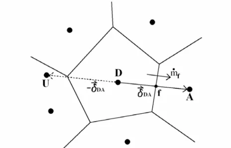
The face value αf can be estimated as a function of neighbor cells. Figure 3.1 shows a control volume and its neighbor cells which determined by flow direction on the control surface. The subscripts U, D and A denote upwind cell, donor cell and accepter cell.
Figure 3.1 the relationship of a control volume and its neighbor cells
directly for a consider face. To discretize the VOF equation, as will be seen in section 3.5, the value of α at each cell face need to be estimated by some approximations and then the value of upwind cell αU will be obtained. The most convenient way to estimate the face value
f
α is either the upwind difference scheme or the central difference scheme. These two schemes can be combined as:
(
)
⎟ ⎠ ⎞ ⎜ ⎝ ⎛ − + = ⇒ ⎟ ⎟ ⎠ ⎞ ⎜ ⎜ ⎝ ⎛ − + + − + = 2 2 D A D f D D A D UD CD UD f α α γ α α α α α γ α α α γ α α = (3.1)The second term of the right-hand-side stands for an anti-diffusion correction to the upwind differencing. This approximation becomes central differencing for γ =1, which may cause oscillations in the region of large gradients. To ensure boundedness of solution γ must be limited. The families of schemes based on the Total Variation Diminishing (TVD) [16] flux limiters are examples of this approach. Furthermore, these schemes are implemented in the context of the normalized variables formulation (NVF) which is proposed by Leonard [16] for the development of normalized variables diagram (NVD) schemes originally. Sweby [22] presented the limiter γ as a function of the ratio of two consecutive gradients r :
D A U D
r
α
α
α
α
−
−
=
(3.2)The volume fraction value can be normalized as:
U A U α α α α α − − = ~ (3.3)
The normalized variable can be used to give expressions for α~D and α~ : f
U A U D D α α α α α − − = ~ (3.4)
U A U f f α α α α α − − = ~ (3.5)
With the normalization α~ =U 0 and α~ =A 1.
Introducing normalized variables into equation (3.1) leads to
)
2
~
1
)(
(
~
~
D D fr
α
γ
α
α
=
+
−
(3.6) where D Dr
α
α
~
1
~
−
=
(3.7)It is seen from the above equation, α~ is simply a function of f αD
~ .
3.3 Linear difference schemes
Figure 3.2 shows the Normalized Variable Diagram (NVD) for a number of linear difference schemes. In the Figure the normalized face value is plotted as a linear function of the normalized donor cell value.
Figure 3.2 Normalized Variable Diagram (NVD).
UDS (Upwind Difference Scheme) is unconditionally stable and always produces a bounded solution, but has high numerical diffusion and loses accuracy. DDS (Downwind Difference Scheme) is a first-order scheme that introduces negative numerical diffusion. CDS (Central Difference Scheme), LUS (Linear Upwind Scheme), Fromm’s scheme and QUICK (Quadratic Upwind Interpolation for Convective Kinematics) scheme are second-order
accuracy schemes. The shortcomings of high order schemes are the causes of solution oscillations in sharp gradient regions. In the above diagram, the line of high order schemes would pass the point (0.5, 0.75). As given in equation (3.6), the different scheme at face α~ f
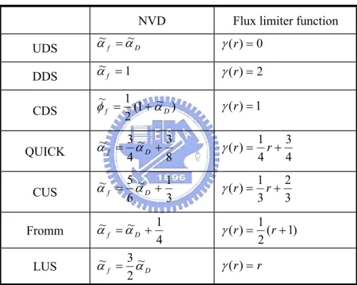
can be written as the combination of the UDS and an anti-diffusive term. Different schemes can be represented by specifying a specific flux limiter γ which is a function of the gradient ratio r . A list of the linear difference schemes is given in the following table. Their relationships are also plotted in Figure 3.3.
NVD Flux limiter function
UDS αf αD ~ ~ = γ(r)=0 DDS α~ =f 1 γ(r)=2 CDS φ~f =21(1+α~D) γ(r)=1 QUICK α~f =43α~D +83 4 3 4 1 ) (r = r+ γ CUS α~f =65α~D +31 3 2 3 1 ) (r = r+ γ Fromm 4 1 ~ ~ = + D f α α ( 1) 2 1 ) (r = r+ γ LUS αf αD ~ 2 3 ~ = γ(r)=r
Table 3.1 The normalized variable (NV) and flux limiter function of linear schemes.
Figure 3.3 Relationship between γ and rfor linear difference schemes.
3.4 Non-linear difference schemes
There are many high-order linear approaches introduced in section 3.1. However these the high-order schemes do not satisfied the Convective Boundedness Criterion (CBC) which was proposed by Gaskell and Lau [23]. The boundedness criterion of CBC can be shown in the NVD (see the shadow area of Figure (3.2)) :
⎪⎩ ⎪ ⎨ ⎧ ≤ ≤ ≤ ≤ > < = 1 ~ 0 1 ~ ~ 1 ~ 0 ~ ~ ~ D f D D D D f for or for α α α α α α α (3.8) To satisfy the CBC, a high-order scheme has to be a non-linear framework. Hence, high resolution schemes (HRS) [20] are developed for solving this problem which have the following properties: (i) solutions are free from oscillations or wiggles, (ii) high accuracy is obtained around shocks and discontinuities and (iii) CBC is satisfied. Non-linear approaches get a flux-limiter function to ensure a bounded value. The schemes of SMART and STOIC are classified as NVD category.
Sweby [22] has shown that the following constraint on the limiter guarantees that the scheme satisfies the TVD condition.
( ) 0 ( f , ( )) 2 f r r r γ γ ≤ ≤ (3.9)
Figure 3.4 shows TVD constraints in NVD and TVD diagram. The hatched region is known as the second-order regime. Therefore, high resolution schemes which pass through the
shadow area of Figure 3.2 satisfy CBC, but not fit in TVD constraints completely. It is apparent that the TVD schemes are more constrained than the NVD schemes. The MUSCL, SUPERBEE, OSHER and Van Leer schemes are developed based on the TVD theory.
(a) (b)
Figure 3.4 TVD Constraints in (a) NVD and (b) TVD diagram.
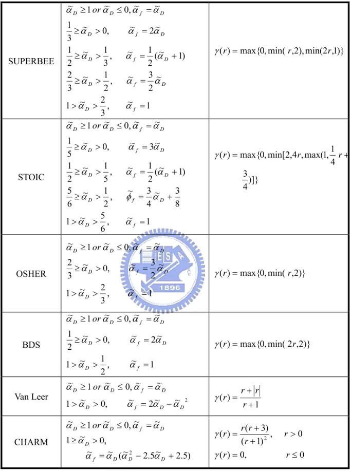
The following table lists the NVD equation and flux limiter equation in TVD of non-linear high resolution schemes.
NVD Flux limiter equation
SMART 1 ~ , 6 5 ~ 1 8 3 ~ 4 3 ~ , 6 1 ~ 6 5 ~ 3 ~ , 0 ~ 6 1 ~ ~ , 0 ~ 1 ~ = > > + = > ≥ = > ≥ = ≤ ≥ f D D f D D f D D f D D or α α α α α α α α α α α α )} 4 , 4 3 4 1 , 2 min( , 0 max{ ) (r = r+ r γ MUSCL 1 ~ , 4 3 ~ 1 4 1 ~ ~ , 4 1 ~ 4 3 ~ 2 ~ , 0 ~ 4 1 ~ ~ , 0 ~ 1 ~ = > > + = > ≥ = > ≥ = ≤ ≥ f D D f D D f D D f D D or α α α α α α φ α α α α α )} 2 , 2 1 2 1 , 2 min( , 0 max{ ) (r = r+ r γ
SUPERBEE 1 ~ , 3 2 ~ 1 ~ 2 3 ~ , 2 1 ~ 3 2 ) 1 ~ ( 2 1 ~ , 3 1 ~ 2 1 ~ 2 ~ , 0 ~ 3 1 ~ ~ , 0 ~ 1 ~ = > > = > ≥ + = > ≥ = > ≥ = ≤ ≥ f D D f D D f D D f D D f D D or α α α α α α α α α α α α α α α )} 1 , 2 min( ), 2 , min( , 0 max{ ) (r = r r γ STOIC 1 ~ , 6 5 ~ 1 8 3 ~ 4 3 ~ , 2 1 ~ 6 5 ) 1 ~ ( 2 1 ~ , 5 1 ~ 2 1 ~ 3 ~ , 0 ~ 5 1 ~ ~ , 0 ~ 1 ~ = > > + = > ≥ + = > ≥ = > ≥ = ≤ ≥ f D D f D D f D D f D D f D D or α α α φ α α α α α α α α α α α )]} 4 3 4 1 , 1 max( , 4 , 2 min[ , 0 max{ ) (r = r r+ γ OSHER 1 ~ , 3 2 ~ 1 ~ 2 3 ~ , 0 ~ 3 2 ~ ~ , 0 ~ 1 ~ = > > = > ≥ = ≤ ≥ f D D f D D f D D or α α α α α α α α α )} 2 , min( , 0 max{ ) (r = r γ BDS 1 ~ , 2 1 ~ 1 ~ 2 ~ , 0 ~ 2 1 ~ ~ , 0 ~ 1 ~ = > > = > ≥ = ≤ ≥ f D D f D D f D D or α α α α α α α α α γ(r)=max{0,min(2r,2)} Van Leer ~ ~ 2 2 ~ , 0 ~ 1 ~ ~ , 0 ~ 1 ~ D D f D D f D D or α α α α α α α α − = > > = ≤ ≥ 1 ) ( + + = r r r r γ CHARM ) 5 . 2 ~ 5 . 2 ~ ( ~ ~ , 0 ~ 1 ~ ~ , 0 ~ 1 ~ 2 − + = > ≥ = ≤ ≥ D D D f D D f D D or α α α α α α α α α ( ) 0, 0 0 , ) 1 ( ) 3 ( ) ( 2 ≤ = > + + = r r r r r r r γ γ
Table 3.2 The NVD equation and flux limiter function of non-linear difference schemes.
Figure 3.5 to 3.11 show the NVD and TVD diagrams of a number of high resolution schemes.
Figure 3.5 SMART
Figure 3.6 MUSCL
Figure 3.8 STOIC
Figure 3.9 OSHER
Figure 3.11 Van Leer
Figure 3.12 CHARM
3.5 The normalized variables for unstructured grids
For the unstructured grids, the upwind value αU is required for variable normalization, but is not readily availiable. A estimation of αU can be obtained with a pseudo-upwind node U located at a distance of negative δDA
v
away from donor node D (see Figure 3.13). Thus,
DA D A
U α α δ
α = −2∇ ⋅ v (3.10)
The above approximation is necessary to be bounded as:
{
}
{
max ,0 ,1}
min U
U α
Figure 3.13. The prediction of upwind value for an arbitrary cell arrangement
3.6
Discretization of the indicator equation
Finite volume method is a popular method in CFD and will be applied in this study. This method uses the integral form of the conservation equations. The solution domain is divided into a finite number of control volumes, and the conservation equations are applied to each control volumes. The finite volume method is suitable for arbitrary geometries and can accommodate any type of grid. The finite volume approach is perhaps the simplest to understand and to program. All terms that need be approximated have physical meaning which is why it is popular with engineers.
The finite volume discretization of the equation (2.13) is performed by taking integration of the indicator equation over a control volume :
0 = ∀ ⋅ ∇ + ∀ ∂ ∂
∫∫∫
∫∫∫
∀ ∀ d V d t r α α (3.12) and then use the Gauss’s divergence theory :0 = ⋅ + ∀ ∂ ∂
∫∫
∫∫∫
∀ S S d V d t r r α α (3.13) The first term at the left-hand-side is an unsteady term and can be discretized by:(
o)
D n D t d t α α α − Δ ∀ Δ ≈ ∀ ∂ ∂∫∫∫
∀ (3.14)where Δ∀ is the volume of the cell and the superscript n and o denoting new-time level and old-time level.
The second term at left hand side of equation (3.14) is the convection term and can be approximated as f f f o S S V S d Vv ⋅ v ≈
∑
v ⋅ v∫∫
(α
) (α
) (3.15)where the subscript f denoting that the properties on the surface of a control volume.
For the discretization, the first-order implicit scheme is computationally robust, stable and efficient, but suffers from numerical diffusion. On the other hand, the first-order explicit scheme is stable only for limited time steps. In the presenting work, we will adopt the second-order Crank-Nicolson scheme with large time steps.
In the equation (3.15), the value αf is approximated by
(
o)
f n f f α α α = + 2 1 (3.16) Substituing above equation and using the apprximation given in equation (3.1) in which the anti-diffusion term is treated as a fully explicity manner, the discretization of indicator equation can be presented as:∑
+ = nb n nb nb n P P A S A α α α (3.17) where t A A nb nb P Δ ∀ Δ + =∑
(3.18) ) 0 , max( 2 1 v nb F A = −& (3.19)( )
(
)
∑
⎢⎣⎡ − − − − ⎥⎦⎤ = nb V D A o P o nb V F r F Sα & α α γ φ φ & 2 ) )( 0 , max( 2 1 (3.20) where F& is the volume flux at each face, the subscript P denote the primary node and nb V3.7 Blending strategy
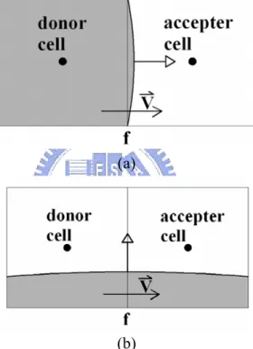
To further enhance accuracy and reduce numerical diffusion and dispersion, composite schemes with blending strategy is introduced. There is a weighting factor based on the angle between interface and direction of motion. If the cell has started to be filled with fluid from the upwind side of the interface and the interface is parallel to the cell face, then only fluid present at the downwind cell should be convected through the cell face. In this case a compressive scheme should be used (see Figure 3.14(a)). However, if the interface is perpendicular to the cell face, a HR scheme would be appropriate (see Figure 3.14(b)).
(a)
(b)
Figure 3.14 (a) the interface is parallel to the flow direction and the compressive scheme will be used (b) the interface is perpendicular to the flow direction and high resolution schemes are appropriate.
The above-mentioned situations represent extreme cases in which the interface is either parallel or perpendicular to the control volume face. In general, the angle between the interface and control volume face is between these two cases. The normalized face value can be written as
( )
f f HR(
( )
f)
e compressiv f f α f θ α f θ α~ = ~ ( ) + ~ ( )1− (3.21)where °≤ ≤ ° ∇ ⋅ ∇ =cos−1 , 0 90 f f f f d d θ α α θ r v
In the equation (3.21), f
( )
θf is a blending function between zero and one.The following will introduce the HRIC, CICSAM and STACS schemes.
HRIC
The high-resolution volume tracking scheme (HRIC) [23] is base on a blending of the bounded downwind (BD in table 3.2) and upwind differencing schemes. The blending factor
( )
ff θ is given by
( )
f cos( f )f θ = θ (3.22)
The normalized form of HRIC is:
( )
( )
(
( )
)
( )
(
( )
)
( )
(
( )
)
[
]
⎪ ⎪ ⎪ ⎩ ⎪ ⎪ ⎪ ⎨ ⎧ > < < ⎪ ⎭ ⎪ ⎬ ⎫ ⎪ ⎩ ⎪ ⎨ ⎧ − − − − + + − + < − + = 7 . 0 , ~ 7 . 0 3 . 0 , 3 . 0 7 . 0 7 . 0 ~ 1 ~ ~ 1 ~ ~ 3 . 0 , 1 ~ ~ ~ ) ( ) ( ) ( ) ( ) ( ) ( ) ( ) ( f UDS f f f UDS f f UDS f f BD f f UDS f f BD f f f UDS f f BD f HRIC f Co Co Co f f f f Co f f α α θ α θ α θ α θ α θ α θ α α (3.23) CICSAMThe Compressive Interface Capturing Scheme for Arbitrary Meshes (CICSAM) [25] scheme is also based on the blending strategy. The HYPER-C scheme and the ULTIMATE-QUICKEST (UQ) scheme are utilized when the cell face is perpendicular to the interface and the UQ employed when the face and the interface are parallel.
The HYPER-C scheme is
⎪ ⎩ ⎪ ⎨ ⎧ < < ⎟ ⎟ ⎠ ⎞ ⎜ ⎜ ⎝ ⎛ ≤ ≥ = 1 ~ 0 , ~ , 1 min 0 ~ 1 ~ , ~ ~ D D D D D f Co or α α α α α α (3.24)
(
)
(
)
⎪ ⎪ ⎩ ⎪⎪ ⎨ ⎧ > > ⎪⎭ ⎪ ⎬ ⎫ ⎪⎩ ⎪ ⎨ ⎧ ⎪⎭ ⎪ ⎬ ⎫ ⎪⎩ ⎪ ⎨ ⎧ + − + ≤ ≥ = 0 ~ 1 , ~ , 1 min , 8 3 ~ 6 1 ~ 8 min 0 ~ 1 ~ , ~ ~ D D D D D D D f Co Co Co orα
α
α
α
α
α
α
α
(3.25) (a) (b)Figure 3.15 The NVD of (a) HYPER-C and (b) UQ at Cof equal 0.5
Therefore, the CICSAM scheme can be written mathematically as
(CICSAM) f HYPER C
( )
f f UQ(
( )
f)
f α f θ α f θ
α~ = ~ ( − ) + ~ ( )1− (3.26)
where the blending factor f
( )
θf is⎥ ⎦ ⎤ ⎢ ⎣ ⎡ + = , 1 2 1 ) 2 cos( min ) ( f f f θ θ (3.27) STACS
The Switching Technique for Advection and Capturing of Surfaces (STACS) [24] scheme selects downwind differencing as compressive scheme and modified STOIC as high resolution scheme.
⎪ ⎪ ⎪ ⎪ ⎩ ⎪⎪ ⎪ ⎪ ⎨ ⎧ > > > ≥ + > ≥ + ≤ ≥ 6 5 ~ 1 , 1 2 1 ~ 6 5 , 8 3 ~ 4 3 0 ~ 2 1 ), 1 ~ ( 2 1 0 ~ 1 ~ , ~ ~ ) (mod D D D D D D D D STOIC ified f or α α α α α α α α α = (3.28)
The blending between the two schemes is preformed using
( )
[
cos4( )]
f f
f θ = θ (3.29)
The normalized variables relationship for the STACS scheme is given by
(STACS) f DD
( )
f f ified STOIC(
( )
f)
f α f θ α f θ
α~ = ~ ( ) + ~ (mod )1− (3.30)
The following Figures 3.16(a), 3.16(b) and 3.16(c) show the relationship between compressive schemes and high resolution schemes given by equations (3.22), (3.27) and (3.28) for the above composite schemes. In Chapter 5, these different blending factors will be compared in test cases.
Figure 3.16a Figure 3.16b
Figure 3.16c
Figure 3.16a, 3.16b and 3.16c show the relationship between two schemes for HRIC, CICSAM and STACS.
Chapter 4 Numerical Method for the Velocity Field
4.1 Introduction
This chapter uses finite volume method to discretize momentum equation and pressure equation. All details of each term will be described. In this study, PISO algorithm is adopted to solve unsteady flow field.
4.2 Discretization
Take volume integral of the the momentum equation (2.5) to yield :
( )
∫∫∫
(
)
∫∫∫
∫∫∫
∫∫∫
∫∫∫
∫∫∫
∀ ∀ ∀ ∀ ∀ ∀ ∀ ∇ + ∀ + ∀ ∇ − ∀ ∇ Γ ⋅ ∇ = ∀ ⋅ ∇ + ∀ ∂ ∂ d gd Pd d d V d t ρ φ φ ρ σκ α φ ρ r (4.1)where φ designates each velocity component. The volume integral of the convection, diffusion and pressure terms can be transform into surface integral by divergence theory as
∫∫∫
∫∫∫
∫∫
∫∫
∫∫
∫∫∫
∀ ∀ ∀ ∀ ∇ + ∀ + − ⋅ ∇ Γ = ⋅ + ∀ ∂ ∂ d d g S Pd S d S d V d t S ρ φ S φ S ρ σκ α φ ρ r v r r v (4.2)In the following the unsteady equation is treated with the use of fully implicit scheme, which is unconditionally stable in the linear analysis and allows larger time steps for unsteady calculation.
Unsteady term
The volume integral of the unsteady term can be discretized as
(
o)
P n P o P t d t φ φ ρ φ ρ − Δ ∀ Δ ≈ ∀ ∂ ∂∫∫∫
∀ (4.3) The old time level term would be absorbed into the source term.Convection fluxes
The surface integral for the convection term can be approximated by
∑
∑
∫∫
⋅ ≈ ⋅ = f C f f f f S F S V S d Vv ) v ( v ) v (ρ
φ
ρ
φ
(4.4) Then, f f c f m F = & ⋅φ (4.5)where m&f is the mass flux through the consider face.
As mentioned in the chapter 3, the convective flux is calculated as:
( )
⎟⎟ ⎠ ⎞ ⎜⎜ ⎝ ⎛ − + = 2 D A D f r φ φ γ φ φ (4.6)where the subscript D denotes the donor node and A the acceptor node. The convetive fluxes at donor node and acceptor node can be calculated as:
⎪⎩ ⎪ ⎨ ⎧ < = = > = = 0 , 0 , f P A nb D f nb A P D m for m for & & φ φ φ φ φ φ φ φ (4.7) In the above the subsript P stands for the primary node, nb the neighbor node (see Figure 4.1) In the momentum calculation the Van Leer scheme is adopted, which is given by
1 ) ( + + = r r r r γ (4.8)
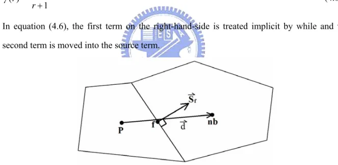
In equation (4.6), the first term on the right-hand-side is treated implicit by while and the second term is moved into the source term.
Figure 4.1 Illustration of the primary cell P and the neighbor cell nb with a consider face f. Diffusion fluxes
The surface integral of the diffusion term is approximated by
(
)
∑
=∑
∇ ⋅ f f f f o f D f S F μ φ r (4.9)Let Srf =dr+
(
Srf −dr)
, when dr is a vector pointing in the direction from primary node toPnb f Pnb f S S d δ δ r r r r r ⋅ = 2 (4.10) The diffusion flux can then be expressed as:
(
)
(
S d)
S S F nbn Pn of of f f Pnb f o f D f r r r r r − ⋅ ∇ + − ⋅ = φ φ μ φ δ μ 2 (4.11) in which the second term at the right-hand-side is also treated explicitly and is moved into the source term.Pressure term
The surface integral is approximated as
∑
∫∫
= =∇ Δ∀ f o f o f s P S P s Pdv r (4.12)Gravitational acceleration term
The gravitational acceleration term can be approximated as
∀ Δ = ∀
∫∫∫
∀ o g d g ρ ρv v (4.13)Surface tension term
The surface tension term in the equation (3.2) can be discreted as:
( )
∇ Δ∀ = ∀ ∇∫∫∫
∀ P P d σκ α α σκ (4.14)As mentioned in the section 2.4, a smooth κ exists in the transitional region where P
( )
∇α P ≠0.The gradient
( )
∇α P is described as:( )
∑
∀ Δ = ∇ f f f P S α α 1 v (4.15)where αf is the face value obtained via the interpolation from the two neighboring node
values.
( )
∑
⎥⎥ ⎦ ⎤ ⎢ ⎢ ⎣ ⎡ ∇ ∇ ⋅ ∀ Δ − = ⎥ ⎥ ⎦ ⎤ ⎢ ⎢ ⎣ ⎡ ⎟ ⎟ ⎠ ⎞ ⎜ ⎜ ⎝ ⎛ ∇ ∇ ⋅ ∇ − = f f f f P P S α α α α κ 1 v (4.16)The face value
( )
∇α f is calculated by interpolating from the neighboring node values.Arrangement of the difference transport equation
The discretized momentum transport equation was approximated can be arranged as ∀ Δ ∇ − + =
∑
o nb n nb nb n P P A S P A φ φ (4.17) in which∑
+ ΔΔ∀ = nb o P nb P t A A ρ(
,0)
max 2 f f Pnb f o f nb m S S A r r & r − + ⋅ = δ μ( )
(
)
(
)
( )
∇ Δ∀ + ∀ Δ + Δ ∀ Δ + ⎭ ⎬ ⎫ ⎩ ⎨ ⎧− − + ∇ − =∑
o P o P o o P f f o f o f D A f g t d S r m S α σκ ρ φ ρ φ μ φ φ γ v r r & 2where the source term S includes old-time level unsteady term, the anti-diffusion term, the cross diffusion term, the gravitational term and the surface tension term.
4.3 Pressure-velocity coupling with PISO
A non-iterative method named PISO which stands for Pressure-Implicit with Splitting of Operators proposed by Issa [23] for unsteady incompressible flow is used in the present study. This breakthrough of PISO is attributed to the few more correctors at each time step while SIMPLE has only one corrector proceeded at each iteration step. PISO involve one predictor step and two corrector steps. It is described in the following.
Predictor step
The predictor step is to solve the momentum equation using the prevailing pressure field.