國立臺灣大學理學院海洋研究所 碩士論文
Graduate Institute of Oceanography College of Science
National Taiwan University Master Thesis
台灣西南海域微量金屬沈積歷史
Historical Record of Trace Metals Offshore Southwestern Taiwan
李純瑜 Chun-Yu Lee
指導教授:蘇志杰博士 Advisor: Chih-Chieh Su, Ph.D.
中華民國 107 年 10 月
October, 2018
誌謝
在讀研究所的路上,真的很幸運能遇到蘇老師,老師在研究上總是給予我們 非常彈性的空間和最大的資源,雖然我總是被死線追著跑,但老師總是盡心盡力 提供他最大的協助,真的非常非常感謝老大。另外還要特別感謝溫老師和小田學 長,沒有你們,我研究所可能要讀 6 年(太衰 XD),所以每次負能爆棚的時候都 會想:大家都盡全力幫妳了,妳還有什麼資格不努力?你們的幫助和支持都是我 前進的動力,真的非常謝謝你們不論是在實驗上或論文寫作上給我的幫助,使我 得以順利完成我的碩士學業。
另外,也非常幸運遇到實驗室的大家,謝謝帶我入門分析化學的 Lulu,從小 豆學長的計畫到自己的實驗,總是耐心幽默的教會我好多事,從完美的滴定到發
現我們都有強迫症(擊掌),讓我跟無塵室變好朋友;305 小家長聖婷和堯禮,總
是在我不知道該怎麼辦時提供貼心意見,並準備食物餵食療癒我們這群孩子(絕
對是畢業後會最想念的溫馨下午茶時光),還有那一同分樣的美好;心思細膩的怡
雯姊,總是貼心的關心提醒,還有超積極的辦事效率,覺得有妳的照顧真好;鳳 心不時暖心的問候和貼心的糖果補給,真的是疲累時的充電能量;半夜研究室大 師兄宇璜的卡農放送(行健說要關燈配合想像自己是居里夫人 XD),著實是首提 高做事效率的經典神曲;還有同學家騏、喆元一起的學習討論還有幫忙;AA 上機 治平的八卦不無聊時光,睿晟的酸,佩俞的手沖咖啡;鶴漢和乒乒在 EGU 幫我拿 到的暖心啤酒;深受學弟愛戴的巴馬策勵我要運動……,還有感謝太多太多的人,
沒有你們,我的研究生活不會如此充實而美滿。
也感謝那些實驗上遇到的不順,讓我學會嘗試自己解決問題、尋求答案,而 且還多學會做不同的儀器,果然多看多學即使失敗卻都還是收穫滿滿。
最後,還是最感謝爸媽的愛與支持,讓我回家可以無憂耍廢盡情享受當爸寶 媽寶的幸福時光,還有那個像是從來沒離開過的你,相信我一路上的幸運,都有 你的 blessing。
中文摘要
台灣位於活動型大陸邊緣,板塊擠壓造山使其發展出眾多高山型小河,這些 河流快速侵蝕地表挾帶大量陸源沈積物傳輸至海洋。自 1970 年代起,台灣工業迅 速發展,1980 年代開始,台灣重金屬汙染問題不斷浮現,甚至擴及沿岸地區,顯 示人為活動已經對臺灣周遭環境造成一定程度的影響。在此地質環境和人為活動 的交互作用下,這些流經高度工業發展和人口居住密集區域的河川,勢必會將這 些經濟發展下對於環境造成負面影響的產物帶進海洋環境當中,此研究目的於探 討這些人為汙染物於海洋沈積物中的堆積歷史紀錄,以了解其傳輸之控制機制、
來源及其擴散影響的範圍。
高屏溪為台灣流域面積最大的一條河流,因流經人口居住密集及工業高度發 展之地區,與其他世界大河相比,擁有顯著高濃度的顆粒態和溶解態金屬。高屏 海底峽谷位於台灣西南海域,其峽谷頭部幾乎與高屏溪連接,為高屏溪帶來大量 陸源物質往深海傳輸的主要通道。本研究主要利用鉛-210 定年、粒徑分析、地化 分析(分析元素包括 Zn, Cr, Pb, Co, Ni, Cu, Cd, Fe, Mn, Al, Ti, Mg, K)等方法,分 析在西南海域周邊採集之岩芯,並以其金屬對 Al 之比值與自然環境(平均上部地 殼、平均臺灣沈積岩、揚子陸塊及平均頁岩)背景值相比,以分辨沈積物中微量
金屬之來源。根據岩心採樣位置,可劃分為三大類:(I)高屏峽谷上段兩側陸坡站
位;(II)高屏峽谷下段深海站位;(III)澎湖峽谷頭部異源站位。
本研究之結果發現在陸棚外之區域找不到顯著的人為汙染訊號,陸棚外大部 分重金屬呈現出相對穩定的時間分佈,其和 Al 的比值皆接近或低於自然背景。然 而,於峽谷上段陸坡站位的表層沈積物中記錄到輕微的 Pb 富集及其隨時間顯著增 加的趨勢,但於深海站並未紀錄到此趨勢,顯示陸源的汙染訊號主要可以到達高 屏陸坡。此外,雖與自然背景並無明顯差異,但在高屏陸坡上這些記錄到 Pb 隨某
段時間劇烈增加的站位中,皆可清楚描繪出台灣工業發展開始的時期(1970 年代)。
除了微量金屬的人為輸入之外,也發現自然災害(地震,颱風等)亦會加速海洋 環境中微量金屬的累積。在高屏陸坡和深海這兩個沈積環境中,兩者擁有相當的 微量金屬累積質量和相對一致的 Ti / Al 莫耳比,顯示這些由高屏峽谷傳輸之沈積
物可以越過陸棚,除了一部分堆積至陸坡,另外也運送相當大量的沈積物至深海 中沈積。雖然沈積物於此研究區跨棚傳輸之特性,使深海成為陸源沈積物的重要 匯區,但在本研究的深海站位並未發現微量金屬的污染記錄,顯示這些陸源之污 染信號可以在進一步向遠洋傳輸的過程中被稀釋,揭示這些汙然源的微量金屬對 於深海的影響是微不足道的。
關鍵字:臺灣西南海域、高屏海底峽谷、汙染歷史、自然災害、傳輸、深海
ABSTRACT
Rapid economic and industrial development over the past five decades in Taiwan has caused the expense of environment. Heavy metals pollution issue has gradually emerged after the 1980s and the contaminated area has extended to the coastal environment. With the tectonic setting and climatic condition in Taiwan, a considerable amount of pollutants could be carried into the marine environment. The aim of this study is to investigate the distribution and transportation of heavy metals through sedimentary records offshore southwestern Taiwan.
Gaoping River (GPR) is the largest river in southern Taiwan and stands out of other major world rivers for its high concentrations of dissolved and particulate metals.
Gaoping Submarine Canyon (GPSC) has been proven to be the major pathway for the transportation of terrestrial materials discharged from GPR into the deep sea. In this study, 210Pb dating, grain size and geochemical analyses (Zn, Cr, Pb, Co, Ni, Cu, Cd, Fe, Mn, Al, Ti, Mg, K) were applied to the sediment cores sampled in three different sedimentary environments around the GPSC: (I) Gaoping Slope sites, (II) Deep sea sites at lower reach of GPSC, and (III) Penghu Submarine Canyon site. Since trace metals could be derived from natural or anthropogenic sources, reference background materials (UCC, ACST, UC-YC and Average Shale) are compared to distinguish the source of the trace metals.
Compared to previous studies conducted in the nearshore regions, pollution signals are hardly to be found in our further seaward sites (Gaoping Slope & deep sea), most of the measured trace metals display a stable temporal distribution with a level near or under the natural background. However, slight enrichment of Pb and its sharp increase
were still recorded within the surface sediments at the Gaoping Slope sites while the records are absent in the deep sea. Moreover, the Gaoping Slope cores which have conformably recorded the pollution of Pb can even clearly illustrate the onset of the industrial development in Taiwan despite their subtle difference from the natural background. Other than the anthropogenic input of the trace metals, natural hazards (earthquakes, typhoons, etc.) are also found to accelerate the accumulation of trace metals in the marine environment. The comparable amount of cumulative mass of the trace metals between Gaoping slope and the deep sea sites and the relatively consistent Ti/Al molar ratio between these two sedimentological regimes, all suggesting that the sediments discharged from GPR could cross the narrow shelf and made a considerable amount to transport and accumulate in the deep sea. Though deep sea can act as an important sink for the terrestrial materials due to the cross-shelf transport, pollution record was not found in the deep sea sites as the pollution signals can be largely diluted during the further seaward transport, implying the pollution in the deep sea is insignificant in the study area.
Keywords: Gaoping Submarine Canyon, Southwestern Taiwan, Trace Metals, Pollution Record, Natural Hazards, Transport, Deep Ocean
CONTENTS
口試委員會審定書 ... #
誌謝 ...i
中文摘要 ... ii
ABSTRACT ...iv
CONTENTS ...vi
LIST OF FIGURES ...ix
LIST OF TABLES ... xii
Chapter 1 Introduction ... 1
1.1 Introduction... 1
1.2 Background ... 2
1.3 Study Area ... 3
1.3.1 Gaoping River (GPR) ... 3
1.3.2 Gaoping Shelf ... 4
1.3.3 Gaoping slope ... 5
1.3.4 Gaoping Submarine Canyon (GPSC) ... 5
1.3.5 Penghu Submarine Canyon ... 6
1.4 Study Aims ... 7
Chapter 2 Sampling & Methods ... 12
2.1 Sampling ... 12
2.1.1 Sampling Sites ... 12
2.1.2 Sampling Method ... 12
2.2 Sample Treatment ... 15
2.3 Analytical Method ... 16
2.3.1 Water Content ... 16
2.3.2 X-Radiography ... 17
2.3.3 210Pb Geochronology ... 18
2.3.4 Grain Size Analysis ... 24
2.3.5 Geochemical Analysis ... 27
Chapter 3 Results and Discussions ... 34
3.1 Sedimentary Properties ... 34
3.1.1 Gaoping Continental Slope Site: S2, S6, S1 and B4G ... 34
3.1.2 Deep Sea Site: MT6 and MT7 ... 36
3.1.3 Penghu Submarine Canyon Site: PL02 ... 39
3.2 Major Element Ratios ... 39
3.2.1 Reference Element (Al) ... 39
3.2.2 Reference Backgrounds ... 42
3.2.3 Ti/Al Molar Ratio ... 50
3.3 Vertical Distribution of the Metals ... 55
3.3.1 S2 (Gaoping Slope Site) ... 55
3.3.2 S6 (Gaoping Slope Site) ... 56
3.3.3 S1 (Gaoping Slope Site) ... 57
3.3.4 B4G (Gaoping Slope Site) ... 59
3.3.5 PL02 (Penghu Submarine Canyon Site) ... 60
3.3.6 MT6 (Deep Sea Site) ... 61
3.3.7 MT7 (Deep Sea Site) ... 63
3.4 Source of the Elements ... 64
3.5 Enrichment of the Trace Metals ... 69
3.5.1 Mn ... 69
3.5.2 Pb ... 73
3.6 Cumulative Mass of the Trace Metals ... 77
3.7 Lead Pollution in Aquatic Sediments in a global Comparison ... 79
Chapter 4 Conclusion ... 83
REFERENCE ... 85
APPENDIX ... 90
LIST OF FIGURES
Figure 1-1 Schematic block diagram illustrating the tectonic setting of Taiwan and the associated major submarine physiographic units (Yu & Song, 1993). ... 8 Figure 1-2 The sediment dispersal system off southwestern Taiwan (Yu et al., 2009). ... 9 Figure 1-3 The intraslope basins distributed on the Gaoping Slope which are separated by the mud diapiric ridges (Yu & Huang , 2006). ... 10 Figure 1-4 The Gaoping (formerly spelled “Kaoping") Submarine Canyon has two morphologic breaks that separate it into three distinct segments, including upper reach, a middle reach and lower reach (Chiang & Yu, 2006). ... 11 Figure 2-1 Study area and sampling sites. ... 13 Figure 2-2 Flowchart of the sample treatment. ... 16 Figure 2-3 The 226Ra, 222Rn, 210Pb, and 210Po in 238U decay series (Swarzenski, 2014). 19 Figure 2-4 Conceptual illustration of the dominant sources and transport pathways for
210Pb (Swarzenski, 2014). ... 20 Figure 3-1 The X-Radiography, core surface image, and profiles of 210Pb, water content and grain size in core S2. ... 35 Figure 3-2 The X-Radiography, core surface image, and profiles of 210Pb, water content and grain size in core S6. ... 35 Figure 3-3 The X-Radiography, core surface image, and profiles of 210Pb, water content and grain size in core S1. ... 36 Figure 3-4 The X-Radiography, core surface image, and profiles of 210Pb, water content and grain size in core B4G... 36 Figure 3-5 The X-Radiography, core surface image, and profiles of 210Pb, water content and grain size in core MT6. ... 37
Figure 3-6 The X-Radiography, core surface image, and profiles of 210Pb, water content and grain size in core MT7. ... 38 Figure 3-7 The topographic map showing the location of core MT6 and MT7
(modified from 蔡, 2014). ... 38 Figure 3-8 The X-Radiography, core surface image, and profiles of 210Pb, water content and grain size in core PL02. ... 39 Figure 3-9 Vertical distributions of Al with comparison to the clay fraction in each sediment core analyzed in this study. ... 41 Figure 3-10 Down core Ti/Al ratio with comparison to the reference background materials (ACST, UCC, UC-YC, Average Shale) in each sediment core analyzed in this study. ... 46 Figure 3-11 Down core Fe/Al ratio with comparison to the reference background materials (ACST, UCC, UC-YC, Average Shale) in each sediment core analyzed in this study. ... 47 Figure 3-12 Down core Mg/Al ratio with comparison to the reference background materials (ACST, UCC, UC-YC, Average Shale) in each sediment core analyzed in this study. ... 48 Figure 3-13 Down core K/Al ratio with comparison to the reference background materials (ACST, UCC, UC-YC, Average Shale) in each sediment core analyzed in this study. ... 49 Figure 3-14 The Ti/Al molar ratios from the fluvial sediments (temporary sinks) and the surface soils (source materials) along the Gaoping (Kaoping) River drainage (Chen et al., 2013). ... 52 Figure 3-15 The spatial distribution of Ti/Al molar ratio compared to previous studies. 54 Figure 3-16 Vertical distribution of the metals in core S2... 56
Figure 3-17 Vertical distribution of the metals in core S6... 57
Figure 3-18 Vertical distribution of the metals in core S1... 59
Figure 3-19 Vertical distribution of the metals in core B4G. ... 60
Figure 3-20 Vertical distribution of the metals in core PL02. ... 61
Figure 3-21 Vertical distribution of the metals in core MT6. ... 62
Figure 3-22 Vertical distribution of the metals in core MT7. ... 64
Figure 3-23 Scatter plot between concentrations of metals (Mg, Ti, Fe, K, Mn, Zn) and Al for each sample in different sediment cores analyzed in this study. ... 67
Figure 3-24 Scatter plot between concentrations of metals (Cr, Pb, Co, Ni, Cu, Cd) and Al for each sample in different sediment cores analyzed in this study. ... 68
Figure 3-25 Vertical distributions of Mn and Mn/Al ratio with comparison to the natural backgrounds in each sediment core analyzed in this study. ... 71
Figure 3-26 Vertical distributions of Mn and Fe in each sediment core analyzed in this study. ... 72
Figure 3-27 Vertical distributions of Pb and Pb/Al ratio with comparison to the natural backgrounds in each sediment core analyzed in this study. ... 75
Figure 3-28 Temporal variations of Pb in (b) Gaoping Slope compared to that in the (a) Gaoping coastal area (head of GPSC) from previous study (Hung & Hsu, 2004). ... 76
Figure 3-29 Cumulative mass of the metals in the last 150 years in core PL02, S2, S6, MT6, B4G and S1. ... 78
LIST OF TABLES
Table 2-1 The detailed information of the collected cores………...14 Table 2-2 The detailed FAAS (iCE 3000 SERIES, Thermo) analytical protocols for the
analyzed element of Zn and Pb……….31 Table 2-3 The detailed ICP-MS (iCapQs, Thermo) analytical protocols for the analyzed element of Mg, Al, K, Ti, Fe, Mn, Cr, Co, Ni, Cu, Cd…………..31 Table 2-4 The concentrations of the standard used to build the calibration line for each
element in FAAS (iCE 3000 SERIES Thermo) and ICP-MS (iCapQs, Thermo)………32 Table 2-5 The results of the Certified Reference Material PACS-3 analyzed in the
study………..33 Table 3-1 The mean major element/Al mass ratios compared to previous study by Chen & Selvaraj (2008) and the reference materials (UCC, ACST, UC-YC, and Average Shale)………...44 Table 3-2 The background ratios of M/Al in different reference materials used in this
study………..45 Table 3-3 The mean 100Ti/Al molar ratios in surface sediments along the Gaoping dispersal system………53 Table 3-4 Comparison in cumulative mass of the trace metals contributed from
non-event and event period in core MT6 and B4G………...79 Table 3-5 Estimated increasing rate of anthropogenic Pb flux in different aquatic
sediments around the world………..82
Chapter 1 Introduction
1.1 Introduction
Trace metals present a trace concentration in the environment matrices. Some of them are vital elements for living organisms, though when they exceed certain threshold concentrations in the environment they can be toxic/noxious and play a threat on lives of either plants or animals (Järup, 2003; Nagajyoti et al., 2010). It has been acknowledged that some of these metals have many adverse health effects and can exist in the environment for a long period of time that can affect the biosphere and hydrosphere. With the global development of industrialization and urbanization, the anthropogenic input of heavy metals has sharply increased in the last century, which makes metal contamination become an important issue worldwide. These metals will not be removed by natural degradation processes, and they can be accumulated in the environment over time, which makes them become a special group of pollutants and deserve a great concern.
Either natural processes or anthropogenic activities could bring metals into the marine environment. The metal elements can be easily adsorbed onto the surface of particles associated with the organic material and can be transported and deposited to the underlying sediments. They are introduced to the marine sediment system through several pathways, including direct terrestrial input from rivers, air deposition, and scavenging from the water column, among which, the riverine input is generally the major source, and can bring a tremendous amount of these metals into the marine environment.
After deposition, distributions of the metals can be modified again by the
post-depositional processes, such as bioturbation, sediment mixing, anomalous sedimentation events (slumps and gravity flows), and diagenesis in the sediments (Finney & Huh, 1989; Zwolsman et al., 1993). Through these complicated processes, the ocean can serve as a final sink for these trace metals. With studying the marine sediments, we could extract the information from sediment records for knowing the influence of surface runoff, the interaction between terrestrial and marine materials and the anthropogenic impacts on the environment.
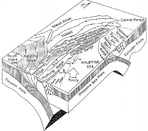
1.2 Background
Taiwan is located on a collision boundary of the Eurasian Plate and Philippine Sea plate, which formed the fold-and-thrust mountain belt and developed many small mountainous rivers on the island (Figure 1-1). Compared to other river basins with different elevations of headwaters in the world, Milliman and Syvitski (1992) suggest these tectonic-generated small mountainous rivers can deliver a much tremendous amount of sediments to the sea and the sediments were more liable to escape from narrow continental shelves to deep waters. Ranged in the latitude of subtropical/ tropical and western edge of Pacific Ocean, Taiwan is deeply influenced by the East Asia monsoon and tropical cyclone system. Kao and Milliman (2008) also point out the importance of earthquakes and typhoons induced episodic events under the tectonic setting and climatic condition of Taiwan and reveal the potential impacts on the river discharge and yield from human activities.
Since the 1970s, Taiwan has experienced a rapid economic and industrial development which subsequently brought a negative impact on the environment. After the 1980s, the problems of heavy metal pollution gradually emerged, and many coastal
areas in western Taiwan have been found contaminated with different heavy metals to some extent. It indicates the contaminated area has expanded to the coastal environment and a considerable amount of trace metals might further be brought to the offshore environment. Thus we would like to know whether these man-made pollutants would be continued transport into the deep sea and be recorded (accumulated) in the marine sediments, or they will be buffered by the great natural pool, ocean, through some geochemical processes.
1.3 Study Area
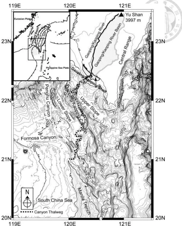
The seafloor morphology off southwestern Taiwan comprises the Gaoping Shelf and Gaoping Slope and finally descends to a water depth of more than 3000 m in the northern end of the abyssal basin of South China Sea. The study area is mainly along the path of Gaoping Submarine Canyon (GPSC) offshore southern Taiwan. The GPSC, which developed on the active continental margin, is the largest submarine canyon system in this geographic area and serves as an active conduit for transporting the terrestrial sediments from Gaoping River to the abyssal plain (Liu et al., 2002; Huh et al., 2009; Yu et al., 2009; Su et al., 2018). Together with the source from the Gaoping River, and pathway cutting through the Gaoping Shelf and Gaoping Slope, they constitute the sediment dispersal system off southwestern Taiwan (Figure 1-2).
1.3.1 Gaoping River (GPR)
The Gaoping River (GPR) is the largest river in southern Taiwan with a drainage area of 3257 km2. Originated from the southern part of the Jade Mountain, it has a mainstream of 171 km and a relatively high average slope gradient of 1/150
(Hydrological Yearbook of Taiwan, 2017). The GPR system is composed by five major tributaries, including Cishan River, Laonong River, Baolai River, Chukou River and Ailiao River. Among them, Cishan River and Laonong River are generally considered as the primary stream of the river system which contribute over 70% of the annual discharge. Two hydrological seasons can be derived from the monthly runoff distribution of GPR. The dry season is from November to April, and due to southwest monsoon and typhoon activities, the wet season is mainly from May to October.
Consequently, the wet season accounts for over 90% of the annual rainfall (~3000 mm/year) in the river basin. The relatively high slope gradient and high precipitation rate of the GPR system also make it as one of the highest physical denudation rates (10934 ton/km2 year) area in the world (Li, 1976; Chung et al., 2009).
Gaoping River flows through densely populated areas and industrial districts in the lower watershed, and the lower part of GPR is heavily polluted due to the discharge from metal scrap factories and livestock farms. As a result, the GPR is not only one of the most contaminated rivers in Taiwan, if compared to other major world rivers, GPR can also present as a prominent role for its high concentrations of either dissolved or particulate metals (Hung & Hsu, 2004). According to Doong et al. (2008), very high concentrations of Cr, Cu, Ni, Zn were detected in the sediments from GPR due to the discharge from swinery and industrial wastewaters.
1.3.2 Gaoping Shelf
The Gaoping Shelf is an offshore extension (progradation) from the sediments progressively deposited seaward from the Pingtung Plain (Yu & Chiang, 1997). It has a length of 100 km that extends northward from the southern tip of the Hengchun
and finally reaches its northern end at the mouth of Tsengwen River (Yu & Chiang, 1997). It is characterized with a narrow platform (20 km wide, a factor of 2-4 narrower than the average width of shelves worldwide) and shallow waters (80 m deep), while having an average slope gradient of 5 m/km which is greater than that (2.5 m/km) of the shelves around the world (Yu & Chiang, 1997). The morphological properties of this shelf are dictated by the tectonic setting of the uplifting Taiwan orogen and the associated sedimentation process.
1.3.3 Gaoping slope
Stretching from the Gaoping Shelf, the Gaoping Slope extends southwestward for a long distance over a broad and deeply sloping region of more than 16000 km2, and finally reachesa water depth of 3500 m (Yu & Song, 1993). An escarpment on the slope ranging at the water depth of 1200 to 2000 m has separated the slope into two parts with an immediate relief over 800 m, producing a steep upper slope and a gentle lower slope (Yu & Song, 1993; Chiang & Yu, 2006). The irregular topography on the slope is the interplay results of deformations of folding, faulting and mass wasting, and silts and clays are the main constitutes in this physiographic region (Yu & Song, 1993; Chiang &
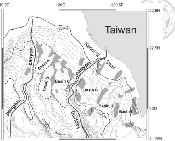
Yu, 2006). Mud diapirs were discovered widely distributed on this slope region, forming intraslope basins between these structural highs, and a distinct upward series of seismic facies can be found over the sedimentary processes in these basins (Figure 1-3, Yu &
Huang, 2006).
1.3.4 Gaoping Submarine Canyon (GPSC)
Gaoping Submarine Canyon begins immediately with the river mouth of GPR,
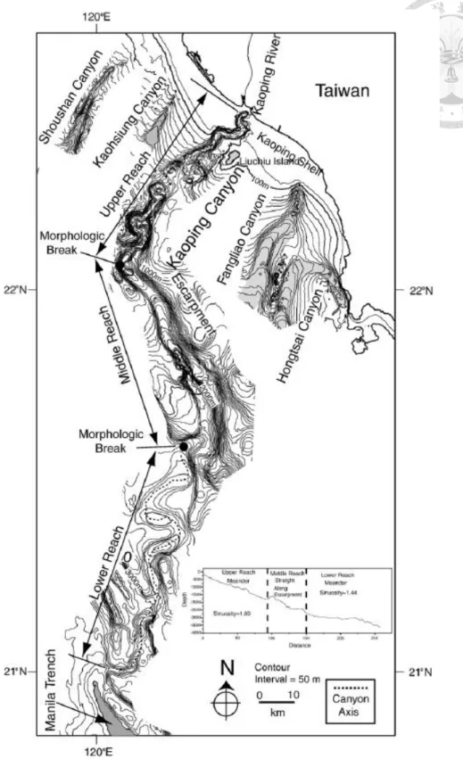
crossing through the narrow Gaoping shelf and the broad Gaoping slope, and finally emerging into the northern end of Manila Trench with a length of 260 km (Chiang & Yu, 2006). According to the morphological features of GPSC controlled by tectonics and structures, it can be divided into three distinct segments, including upper reach, a middle reach and lower reach (Figure 1-4). The upper reach cutting through the shelf and the upper slope meanders towards southwest with a distance of 88 km to a water depth of 1600 m (Chiang & Yu, 2006). With a sharp bend from the upper reach, the middle reach presents a nearly linear southeast orientation along the foot of the escarpment with V-shaped valley and extends for a distance of 65 km to a water depth of 2600 m (Chiang & Yu, 2006), and be consider as either a temporary sediment sink or conduit (Yu et al., 2009). The lower reach finally turns back toward the southwest direction on the lower slope and elongates with a distance of 100 km where it emerges into the northern end of Manila Trench at the water depth of 3500 m (Chiang & Yu, 2006). Previous geophysical study along this canyon suggests that the recurrent hyperpycnal flows in the GPSC can be an important force to erode Gaoping Shelf and Gaoping Slope and brought the eroded sediments continually transported to the deep sea (Yu et al., 2009).
1.3.5 Penghu Submarine Canyon
Eastern to the GPSC, there lies another submarine canyon, Penghu Submarine Canyon, which separates the Gaoping slope and the South China Sea slope. It has a length of 180 km from its head started from the shelf break of the Taiwan Strait Shelf to its mouth emerging into the Manila Trench. Unlike most of the submarine canyons developed on submarine slopes with heads normal to the shoreline, Penghu Submarine
reach and a lower reach demarcated by a clear knickpoint occurred at the water depth of 2500 m and about 100 km away from the canyon head along the longitudinal axis of the canyon. Above the knickpoint, the upper reach displays a fan-like network with 3 major tributary canyons, which is characterized with a steep slope (1.42 degrees), V-shaped valleys, and high relief from the edge to the bottom of the canyon, showing a greater intensity of erosion and represents a typical canyon morphology. The lower reach shows to have only one single course without any tributary canyons and occurred on a gentle slope angle of 0.5 degrees, having broad U-shaped troughs and relatively small relief between the edges and bottoms of the canyon. These morphological properties of the lower reach canyon imply a low-intensity downward erosion and mild structural uplift by thrust faults (Yu & Chang, 2002). Penghu Submarine Canyon is also an important conduit for bringing the orogenic sediments from Taiwan and sediments from passive Chinese margin together to sink into the Manila Trench (Yu & Chang, 2002).
1.4 Study Aims
According to Hung & Hsu (2004), the surface sediments at Gaoping coastal area (near the mouth of GPR) have been largely contaminated with trace metals (Pb, Zn, Cr, Ni, Cd), and GPSC appears to be the major sink for river borne trace metals. By comparing to several published reference materials in major element ratios and applying the factor analysis, Chen & Selvaraj (2008) access the contamination at the (iron and steel) slag-dumping area offshore southwestern Taiwan and reveal the sources and dominated geochemical associations of the elements. Previous studies about the metal distributions and contaminations in sediments off southwestern Taiwan only concentrated on the nearshore regions, while seldom has focused on the influence of
heavy metals in further seaward areas (e.g. lower slope, deep sea basin). Therefore, the study will focus on the areas on the Gaoping Slope and the deep sea basin along the Gaoping Submarine Canyon. The objective of this study is to determine the concentrations and the fate of the metals and the transport mechanisms through the sedimentary records off southwestern Taiwan.
Figure 1-1 Schematic block diagram illustrating the tectonic setting of Taiwan and the associated major submarine physiographic units (Yu & Song, 1993).
Figure 1-2 The sediment dispersal system off southwestern Taiwan, consisting of the Gaoping River (GPR), the Gaoping Shelf, the Gaoping Slope, and the Gaoping Submarine Canyon (GPSC) (Yu et al., 2009).
Figure 1-3 The intraslope basins distributed (determined by seismic profiles) on the Gaoping Slope which are separated by the mud diapiric ridges (Yu & Huang , 2006).
Figure 1-4 The Gaoping (formerly spelled “Kaoping") Submarine Canyon has two morphologic breaks that separate it into three distinct segments, including upper reach, a middle reach and lower reach (Chiang & Yu, 2006).
Chapter 2 Sampling & Methods
2.1 Sampling 2.1.1 Sampling Sites
The sampling sites are mainly along the Gaoping Submarine Canyon which has been proven to be the major pathway for the transportation of terrestrial materials brought by Gaoping River into the deep sea (Liu et al. 2002; Huh et al. 2009; Su et al.
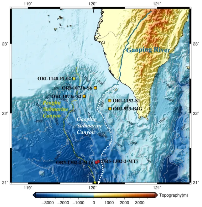
2018). Since the purpose of this study is to establish the historical record of trace metals, the sampling sites were chosen at flank of GPSC where is relatively stable and can provide a better age model for sedimentary history reconstruction. The sampling sites (Figure 2-1) represent 3 major geographic zones, including the Gaoping Slope (sites on the Gaoping Slope at lateral sides of the upper reach of GPSC, yellow squares in Figure 2-1, including S6, S2, S1 and B4G), the Penghu Submarine Canyon (a site located on the Palm Ridge at the head of Penghu Submarine Canyon, green square in Figure 2-1, PL02) and deep ocean (sites at lower reach of the GPSC with water depth over 2600m, red squares in Figure 2-1, including MT6 and MT7). The details of the sampling sites are shown in Table 2-1.
2.1.2 Sampling Method
7 sediment cores were collected by using gravity corer and piston corer on R/V Ocean Researcher 1 and R/V Ocean Researcher 5 from 2010 to 2016. Core information (core top, core length, cruise number, and station name) were marked on the core tube upon collection, and the sediment cores were immediately stood upright until the
were removing the sea water on the core tope, cutting the tube into a proper length (<150 cm), and filling the hollow space with plastic wrap covered styrofoam to prevent the disturbance of the sediments. Both ends of the sediment cores were capped by a lid with tape sealed to prevent the loss of water contained in the sediments.
Figure 2-1 Study area and sampling sites. The collected sediment cores are from three different geographic locations: (I) Gaoping Slope (S2, S6, S1 and B4G, yellow square in the map), (II) Deep Sea (MT6 and MT7, red squares in the map), and (III) Penghu Submarine Canyon (PL02, green square in the map).
Gaoping Submarine Canyon Penghu
Submarine
Canyon
Table 2-1
The detailed information of the collected cores.
Cruise Station Water Depth (m)
Sampling Time (GMT+8)
Longitude Latitude Core Length
(cm)
Core Type
210Pb & Grain Size Data
Source ORI-1148 PL02 931 2016/10/04
12:30 119°42.74' 22°30.05' 114 GC (林等人, 2016) ORI-1073a S2 1205 2014/05/09
06:15 119°52.218' 22°14.815' 123 GC (徐, 2015)
ORI-1073b S6 618 2014/05/14
22:36 120°02.58' 22°22.02' 112 GC (徐, 2015)
ORI-1152 S1 822 2016/11/02
03:38 120°15.87' 22°11.03' 93 GC -
ORI-923 B4G 863 2010/04/06
07:28 120°16.20' 22°04.04' 67 GC (鄭, 2012) OR5-1302-2 MT6 3078 2013/03/06
20:00 120°03.61' 21°17.52' 91 PC (蔡, 2014) OR5-1302-2 MT7 2654 2013/03/07
02:48 120°05.32' 21°18.27' 498 PC (蔡, 2014) GC: Gravity Core ; PC: Piston Core.
2.2 Sample Treatment
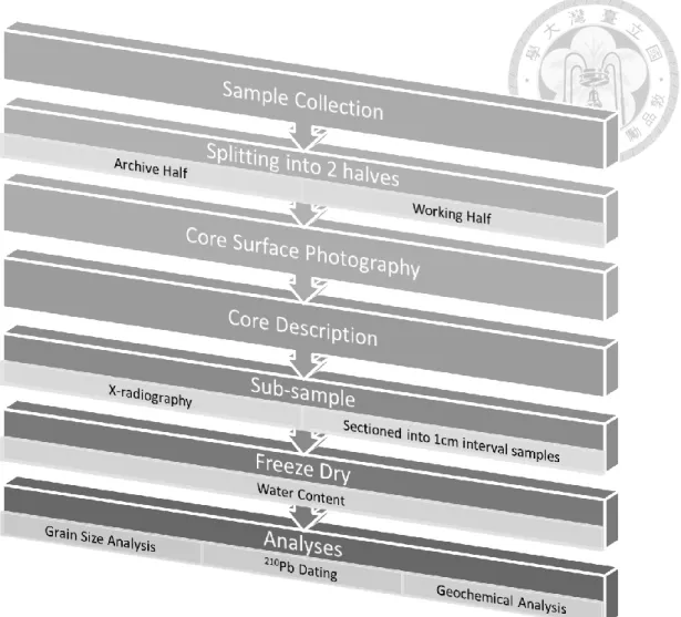
The sediment cores were sent to the Taiwan Ocean Research Institute (TORI) for preliminary treatments, including core splitting (splitting the core samples into two halves, as working and archive halves, respectively), core surface photography, core description, and Multi-Sensor Core Logger (MSCL) scan. The working halves were taken back to Marine Sedimentology and Environmental Radioactivity Lab (MSERL) at IONTU for subsequent core analysis processing, including sliced working half cores into 1 cm thickness by using a transparent acrylic slab (25 × 10 × 1 cm) for X-ray photography while the rest core sample was sliced into 1 cm interval and stored in 50 mL centrifuge tube. The samples were freeze-dried for 3-5 days prior to the following analyses. The analytical process is shown as Figure 2-2.
Figure 2-2 Flowchart of the sample treatment.
2.3 Analytical Method
Analytical methods of sediment samples using in this study include X-radiography,
210Pb geochronology, laser grain size analysis and geochemical analysis (determine the concentrations of Zn, Cr, Pb, Co, Ni, Cu, Cd, Fe, Mn, Al, Mg, K, Ti).
2.3.1 Water Content
The water content in the sediments is the proportion of pore water in the sediments.
The pore water was removed from the sediments by freeze-dryer, which applies the
condensation and vacuum state to make the water sublimate into gas and flee away from the sediments. After the wet weights of sediment samples were recorded, 1cm-interval sectioned sediments were fully frozen.
A freeze-dryer produced by Kingmech company is used to remove the pore water within the sediments, at the setting of -55°C, vacuum 30-50 millitorr (1 atm = 760000 millitorr) for 3-4 days. The water content is calculated as below:
water% = 𝑊𝑤𝑒𝑡− 𝑊𝑑𝑟𝑦
𝑊𝑤𝑒𝑡− 𝑊𝑡𝑢𝑏𝑒× 100%
where 𝑊𝑤𝑒𝑡 is the weight of wet sediment in the centrifuge tube, 𝑊𝑑𝑟𝑦 is the weight after being freeze-dried, and 𝑊𝑡𝑢𝑏𝑒 is the weight of the centrifuge tube without sediment sample.
2.3.2 X-Radiography
Hamblin (1962) first used the technique of X-ray photography for studying micro structures of sandstone and siltstone, followed by Calvert and Veevers (1962) to apply this method to unconsolidated marine sediments. Bouma (1964) later facilitated this method and discuss the sedimentary features obtained from this technique in different sedimentation environments. This technique allows us to build up an integrated structural picture of sediment core and provide us information for examining the homogeneity of the sample, and even reveals some latent structures lied within the sample, through, a non-destructive way.
In this study, AXR Model M160NH Cabinet X-ray System was employed to obtain the sedimentary structural pictures of the sediment samples. The 1 cm thick sediment slab (surface polished) was placed in the scan room for the X-ray exposure with the X-ray operating settings of 60-70 keV and 2-3 mA, and integration (exposure) time of
100-140 ms, all of which were adjusted in regard to the properties of the sample.
The X-radiograph image presents the sedimentary features which we can not see through our bare eyes and the primitive information about the cores through the lux of the image which is influenced by physical properties of sediments, such as density and grain size. Bioturbation or some subtle structures (mottles, streaks, etc) hidden in the sediment then can be revealed.
2.3.3
210Pb Geochronology
210Pb is a naturally occurring nuclide from the 238U decay series and has a half-life of 22.23 years (Figure 2-3). Derived from 226Ra (t1
⁄2 =1600 year), 210Pb has a relatively short half-life that makes them reach a radioactive secular equilibrium if the environmental system remained “closed” for a sufficient long time. However, in more recent deposited sediment, there will exist a disequilibrium due to the natural processes, like weathering, transportation and deposition. Since the disequilibrium once formed, they would tend to restore a new radioactive equilibrium which is controlled by their respective decay rate. Such radioactive properties render these nuclides as a useful time-measuring tool (Ku, 1976; Swarzenski, 2014).
The disequilibrium state of 210Pb in a sedimentation system was caused from the additional source of 210Pb. In general, the observed 210Pb in the sediments can be divided into two parts. One part is produced from the intrinsic decay of 226Ra in sediments, representing the time-independent “supported” 210Pb (210𝑃𝑏𝑠𝑢𝑝𝑝𝑜𝑟𝑡𝑒𝑑). The other is considered as the “excess” 210Pb (210𝑃𝑏𝑒𝑥𝑐𝑒𝑠𝑠) sourced from: (1) the decay of atmospheric 222Rn which gets into the sedimentation system through a wet/dry deposition, (2) the riverine input, and (3) the decay of the 226Ra in the water column
which enters the sedimentation system through rapid scavenging processes (210Pb is a particle-reactive radionuclide which can be easily adsorbed onto suspended particles) (Figure 2-4). The excess 210Pb therefore provides as a chronometer of the sediments deposited in recent 150 years under ideal depositional conditions. With the excess 210Pb, we can use the time-dependent relationship to calculate the sedimentation rate.
The isotope dilution method, adding 209Po as tracer into each sample, was employed to measure the activity of 210Pb in sediment. Based on the principle that 210Po (t1
⁄2= 138.4 day) and 210Pb can reach secular equilibrium in 2 years, with the α count ratio of 210Po and 209Po and the known activity of the internal yield tracer 209Po, we can obtain the activity of 210Po in the samples and then calculate the activity of 210Pb.
Figure 2-3 The 226Ra, 222Rn, 210Pb, and 210Po in 238U decay series (Swarzenski, 2014).
Figure 2-4 Conceptual illustration of the dominant sources and transport pathways for 210Pb (Swarzenski, 2014).
The analytical procedures of 210Pb in sediments are listed as follow:
i. 0.5 g of sediment sample is placed into a cleaned crucible and record sample weight.
ii. Crucible with the sediment sample is transferred into the drying oven and heated at 105°C for over 6 hours to remove water and the weight of water-free sample is recorded.
iii. The water-free sample in the crucible is placed into the muffle furnace and heated at 550°C for 6 hours to ash the organic materials in sediments. The remaining sample weight is recorded after this process.
iv. Prepare clean Teflon beakers and mark them with sample numbers. Add 100 µ L of
209Po tracer into the beaker (record the “exact” weight of 209Po) and transfer the
sample into the beaker (residual sediment in the crucible is rinsed out by ultrapure water).
v. Place the Teflon beakers on the hot plate. Add 5 mL HNO3 (Nitric acid 65%, Merck EMSURE®), covered the beaker and heat at 150°C for 1-2 hours for removing the carbonates in sediments. Then add 5 mL HF (Hydrofluoric acid 40%, Merck EMSURE®) and heat overnight at 150°C to destroy the silicates.
vi. Add 2 mL HClO4 (Perchloric acid 70-72%, Merck EMSURE®) and continually heat at 200°C to digest the organic matter.
*Continually heat for at least 12 hours until a clear solution is obtained. Add sufficient HClO4 to accomplish this step until the black solution turned clear.
vii. Remove the lid and evaporate the solution to an incipient dryness (until a yellow jelly-shaped sample appears) and then add little volume of ultrapure water (18.2 MΩ.cm) to swirl it until a clear solution appears again. A few drops of concentrated NH4OH are added to neutralize the solution (testing the pH value with pH-indicator paper) and forming the orange ferrous iron precipitates. Transfer the orange precipitates into a cleaned centrifuge tube (rinse the Teflon beaker for several times to prevent the loss of the sample).
viii. Wash the orange precipitates with ultrapure water (18.2 MΩ.cm) for at least 3 times (each time centrifuged at 4500 rpm for 3 minutes and pour out the clear supernatant) until there’s no smell of the ammonia.
ix. Add 2 mL 9N HCl to dissolve the precipitates and bring the volume to 20 mL with ultrapure water (18.2 MΩ.cm). After shaking the solution, let it sit overnight.
x. Add 1 mL 9N HCl into the solution and shake it till the precipitates totally dissolved. Centrifuge the solution and transfer the clear and yellow solution into a cleaned glass beaker.
xi. Put the glass beaker with sample solution onto the hot plate and add a small spatula of ascorbic acid to form a complex with ferrous iron (Fe2+), thereby preventing its possible interference with the Po plating. After the color of solution turns colorless from the yellow, drop in silver disk to run the plating process at 80-90°C for 2 hours. The time when the Po plating process starts is recorded.
xii. Pick up the silver disk from the solution and rinse it with ultrapure water (18.2 MΩ.cm) and acetone. Store them in a sealed plastic bag before the Alpha measurement.
The measurement was carried out by α spectrometer (OCTETE PC™ ALPHA SPECTROMETER) and the total activity of 210Pb is corrected for the decay of 210Po (from Po plating time to counting time) and 210Pb (from sample collection time to Po plating time), which was calculated as below:
210Pb
total= 𝐶210
𝐶209×𝐴209
𝑊 × 𝑒−𝜆𝑃𝑜−210(𝑡𝑐𝑜𝑢𝑛𝑡𝑖𝑛𝑔−𝑡𝑝𝑙𝑎𝑡𝑖𝑛𝑔)× 𝑒−𝜆𝑃𝑏−210(𝑡𝑝𝑙𝑎𝑡𝑖𝑛𝑔−𝑡𝑠𝑎𝑚𝑝𝑙𝑖𝑛𝑔) 𝐶210 is the α decay counts of 210Po
𝐶209 is the α decay counts of 209Po 𝐴209 is the activity of the spiked 209Po
𝑊 is the weight of salt-free and water-free sediment sample
(the weight was corrected for the salt contents based on the sea water stoichiometry, an average salinity of 35‰ was postulated)
𝜆𝑃𝑜−210 is the decay constant of 210Po (1.829 yr-1) 𝜆𝑃𝑏−210 is the decay constant of 210Pb (0.0311 yr-1) 𝑡𝑠𝑎𝑚𝑝𝑙𝑖𝑛𝑔 is the time of sample collection
𝑡𝑝𝑙𝑎𝑡𝑖𝑛𝑔 is the time when the Po plating process starts
𝑡𝑐𝑜𝑢𝑛𝑡𝑖𝑛𝑔 is the time when the Aphla counting starts
The down core activity of 210Pb (>150 year) could be seen as the supported 210Pb for the excess 210Pb will not be present that it would has decayed out in the deeper sections. In this study, supported 210Pb was calculated as the mean in the core bottom where there are at least 3 sections showing an approximately constant activity.
Therefore, the activity of excess 210Pb can be obtained by subtracting the down core activity of supported 210Pb as:
𝑃𝑏𝑒𝑥𝑐𝑒𝑠𝑠 = 210𝑃𝑏𝑡𝑜𝑡𝑎𝑙 −210𝑃𝑏𝑠𝑢𝑝𝑝𝑜𝑟𝑡𝑒𝑑
210
For sedimentation rate calculation, we use the advection-diffusion model with the assumption of both the flux of 210𝑃𝑏𝑒𝑥𝑐𝑒𝑠𝑠 to the sediment and sedimentation rate are constant over time, once the sediments deposited (in a closed system) the relationship between 210𝑃𝑏𝑒𝑥𝑐𝑒𝑠𝑠, sedimentation rate and mixing rate can be denoted as:
D𝜕2𝐶
𝜕𝑍2− S𝜕𝐶
𝜕𝑍− 𝜆𝐶 = 0 (2-1)
where Z is the depth of sample (cm or g/cm2), C is the activity of 210𝑃𝑏𝑒𝑥𝑐𝑒𝑠𝑠 at certain depth Z (dpm/g), D is the diffusion coefficient (cm2/yr), S is the sedimentation rate (cm/yr or g/cm2/yr), and λ is the decay constant of 210Pb (0.0311 yr-1). Under the boundary conditions of, (1) the activity of 210𝑃𝑏𝑒𝑥𝑐𝑒𝑠𝑠 at core top (Z = 0) is the initial activity of 210𝑃𝑏𝑒𝑥𝑐𝑒𝑠𝑠 (C = 𝐶0), and (2) the activity of 210𝑃𝑏𝑒𝑥𝑐𝑒𝑠𝑠 will be 0 when the depth reach infinitely large (Z → ∞), if not regarding to the mixing process, the equation (2-1) can be written as:
−S𝜕𝐶
𝜕𝑍− 𝜆𝐶 = 0 (2-2)
the solution of the equation (2-2) is:
ln 𝐶 = ln 𝐶0−𝑍 𝜆𝑆 with the slope of the ln210𝑃𝑏𝑒𝑥𝑐𝑒𝑠𝑠 profile, we can have:
S = −λ slope
where we get the apparent sedimentation rate S. In this study, the slope was obtained from the points in the upper layer based on linear least square fit where the mixing or turbidite layers were excluded.
2.3.4 Grain Size Analysis
Particle size of sediment is an important indicator of hydrodynamic conditions, transport distances, and deposition environments. Early methods for measuring particle size include sieving, settling tubes, and microscope observations. Now, a laser granulometer has been well-developed and widely-used. This laser diffraction technique is based on the principle that particles passing through a laser beam will scatter light at an angle and diminish the light intensity, both of which are related to the particle size. In this study, the grain size analysis was carried out using Laser Diffraction Particle Analyzer (Beckman Coulter LS13 320) equipped with auto-sampler with a detection range of 0.375-2000 µm (11.38--1φ). To plot the graph of grain size distribution, a grade scale mostly used in sedimentological studies is to normalize the grain size to a logarithmic scale, for which the well sorted single-population sediments will present as nearly symmetrical Gaussian probability curve. Therefore, the particle size is generally represented in unit of φ, with numerical conversion to international length unit as: φ =
− log2𝐷 (D is the diameter of the particle in mm).
The measured sediment samples will be pre-treated to remove sea salt, organic
matter and carbonates, and finally followed an addition of 1% sodium hexametaphosphate as a dispersant. These pretreatment steps are to ensure that organic matter and carbonate bodies (for example, foraminifera) do not affect the silicate particle size determination. The pre-treatment procedures are listed as follow:
i. Put about 0.5 g (depending on estimated sand content) sediment sample into a 50 mL centrifuge tube.
ii. 30 mL of RO water is added into the tube and fully mixed with sediments through shaking. Subsequently, this sample is centrifuged for 5 minutes at 4500 rpm and then removing the supernatant. Repeat the process for 3 times to wash out the sea salt.
iii. Add 10 mL 15% H2O2 and shake (loose the cap after shaking) to be well mixed.
Then put the tubes into the ultrasonic bath to let it react for 1-2 days for removing the organic matter. If the reaction is not completed, repeat this step. After the process is completed, wash the sample with RO water for 2 times.
iv. Add 7.5 mL 15% HCl and shake (loose the cap after shaking). Then put the tubes into the ultrasonic bath for 4 hours to remove the carbonates. If the reaction is not completed, repeat this step. After the effervescence is completed, wash the sample with RO water for at least 3 times (testing the pH value with pH-indicator paper).
v. Add 10 mL dispersant (1% sodium hexametaphosphate) into the sample and shake before measurement.
Calculation of particle size statistical parameters (mean, sorting, skewness, kurtosis) can be divided into graphical method and moment method. In this study, the statistical parameters are performed by using moment method which brings the entire frequency
distribution into the determination rather than a few selected percentiles. Method of moments is calculated as below:
Mean = x =∑ 𝑓𝑚𝜑
∑ 𝑓 (1st moment)
Sorting = σ = √∑ 𝑓(𝑚𝜑− 𝑥)2
100 (2nd moment)
Skewness =∑ 𝑓(𝑚𝜑− 𝑥)3
100 ∗ 𝜎3 (3rd moment)
Kurtosis =∑ 𝑓(𝑚𝜑− 𝑥)4
100 ∗ 𝜎4 (4th moment)
where f is the frequency (%) for each size class, and 𝑚𝜑 is the midpoint of each φ class.
According to Folk (1966), the geological meanings of the parameters are as follow:
Median (D
50): Median value of cumulative particle size distribution which is less
susceptible to maximum or minimum values than the average (mean) particle size.Sorting: The standard deviation (σ) of the particle size distribution, which also
represents the degree of dispersion of the particle size in the sediments. The higher value reveals a worse sorting.Skewness: The measure of asymmetry of the particle size distribution. A dominant
population of coarse or fine grains will deviate the distribution curve away from a normal distribution (growing “tail” at one end of the distribution curve).Kurtosis: The measure of peakedness of the particle size distribution. The size
difference between two populations in a mixture will determine the distribution that goes to platykurtic (two equivalent population size) or leptokurtic (two very different2.3.5 Geochemical Analysis
The elements measured in this study include Mg, Al, K, Ti, Fe, Mn, Zn, Cr, Pb, Co, Ni, Cu, Cd. The total concentration of the above metals were determined after digestion of the sediment samples. Measurement was performed on the acid-digested sediment solutions. Flame Atomic Absorption Spectrometer (FAAS) and Inductively Coupled Plasma Mass Spectrometer (ICP-MS) were employed to determine the total content of the elements in the sediments and ensure the accuracy of the data set in this study.
(1) Sample Pre-treatment (Removal of Sea Salt)
The sediments were washed by ultrapure water (18.2 MΩ.cm) to remove any remaining sea salt and then freeze-dried before digestion. About 0.5 g of the sediment sample was transferred into a 50 mL polypropylene centrifuge tube (BD Falcon™) by a plastic spatula. 40 mL of ultrapure water (18.2 MΩ.cm) was also added to the tube and fully mixed with sediment through shaking. The sample was centrifuged for 5 minutes at 4500 rpm and the supernatant was removed. Repeat the process for 3 times and then this washed sediment sample was brought to freeze-dry for 3 days.
(2) Total Digestion
The pre-treated sediments were placed in drying oven overnight to remove water content prior to total digestion. The sediments were digested with multiple acids (HNO3, HF and HClO4), and the procedure is shown as below:
i. Put 0.5 g of the pre-treated (salt-free and water-free) sediment into a cleaned Teflon beaker.
ii. 5 mL of HNO3 (Nitric acid 65%, Merck EMSURE®) is added to the sample and heated on the hot plate at 150°C for 2-3 hours with lid.
iii. Add 5 mL of HF (Hydrofluoric acid 40%, Merck EMSURE®) to the sample with continually heating overnight with lid.
iv. Add 0.5 mL of HClO4 (Perchloric acid 70-72%, Merck EMSURE®) to the sample and heated at 200°C overnight with lid.
*add sufficient HClO4 and heated for a sufficient reaction time until a clear solution was obtained.
v. Remove the lid to evaporate the solution to dryness (until it turns into a white biscuit).
*knock the beakers throughout the process to make the droplets on the beaker wall fall onto the beaker bottom, ensuring the whole sediment solution is all dried and condensed onto the white biscuit.
vi. Add little volume of ultrapure water (18.2 MΩ.cm) onto the white biscuit and add 5 mL of HNO3 (Nitric acid 65%, Merck EMSURE®) to re-dissolve it. This solution was then boiled at 150°C for 1 hour with lid.
vii. Take the solution sample off the hot plate and let it cool for 1 hour.
viii. Put the solution into a 30 mL PP vial and bring the weight to about 25 g by adding ultrapure water (18.2 MΩ.cm).
*the lid and the interior wall of the beaker are washed by ultrapure water (18.2 MΩ.cm) and the beaker is swirled throughout the process to make the wall of the beaker clean and to prevent the loss of the sample.
**all the Teflon beakers should be cleaned by adding 5 mL of HNO3 (Nitric acid 65%, Merck EMSURE®) through boiling with lid at 200°C for 2 hours. And the acid-washed
beakers are then rinsed by ultrapure water (18.2 MΩ.cm) and get fully dried before usage.
**all the PP vials for storing the digested samples should be soaked in 10% (v/v) HNO3
for 3 days, triple-rinsed by ultrapure water (by Merck Millipore Milli-Q-Pod®) and dried in the hood in the clean room before usage.
**Each acid-digested sample was measured in weight unit (wt%), which was then converted into volumetric concentration (g/mL) by its density (obtained from the weight measured during the dilution step).
(3) Measurement
The concentrations of the elements were determined by external standard method using the ICP element standard solutions (Merck). Digested sample solutions were diluted (with 2% HNO3 solution) to ensure that the measured results fall in the linear dynamic range of calibration curve. The linear dynamic range of the calibration curve for each element is shown in Table 2-4. The diluted sample solutions were analyzed using FAAS (iCE 3000 SERIES, Thermo) from Professor Liang-Saw Wen’s Lab in IONTU and ICP-MS (iCapQs, Thermo) from the Exploration & Development Research Institute, CPC, analyzed by In-Tian Lin, see the analytical settings in Table 2-2 and Table 2-3.
**All the dilution procedure was conducted in the clean room.
**All the PE vials for storing the diluted samples should be soaked in 10% (v/v) HNO3
for over 3 days and then triple-rinsed with ultrapure water (by Merck Millipore Milli-Q-Pod®) and dried in the hood of clean room prior to use.
**The diluent 2% HNO3 solution is diluted from the ultrapure nitric acid (Nitric Acid
ULTREX®II Ultrapure Reagent, J.T.Baker)
**Multi-element mixed external standard solutions were prepared from 1000 mg/L of the following ICP element standard solutions from Merck company:
a. Certipur®ICP multi-element standard solution IV, MERCK
1000 mg/L: Ag, Al, B, Ba, Bi, Ca, Cd, Co, Cr, Cu, Fe, Ga, In, K, Li, Mg, Mn, Na, Ni, Pb, Sr, Tl, Zn (23 elements in diluted nitric acid) (contains nitric acid, nickel(II) nitrate)
b. Certipur® Titanium ICP standard solution, MERCK
1000 mg/L: Ti (traceable to SRM from NIST (NH4)2TiF6 in H2O)
(4) Quality Assurance and Quality Control
Quantification of all elements measured in this study was based on calibration lines established by the ICP multi-element standard solutions from Merck. Precision and accuracy of the data were assured through repeated analysis (n =4) of certified reference material PACS-3 (Marine Sediment Reference Material for Trace Metals and other Constituents) from National Research Council Canada (NRC). With the exception of Zn (98%) and Cu (82%), the results for most of the elements are shown within 90 ± 5% of the certified values, see Table 2-5. The precision for the analysis of certified reference material for all elements is better than 5% (all RSD<5%). All samples were measured with 3 replicates and average values are reported. Most (97%) of the reported data lies within 2 standard deviations of the mean, which can empirically account for 95% of probability close to certainty. Repeated analysis of the calibration solution (0.2 ppm) were arranged between every 10-15 samples to monitor the instrumental shift over the duration of measurements and the shift has been corrected.
Table 2-2
The detailed FAAS (iCE 3000 SERIES, Thermo) analytical protocols for the analyzed element of Zn and Pb.
Element Zn Pb
Lamp Current (mA) 75 75
Wavelength (nm) 213.9 217.0
Bandpass (nm) 0.2 0.5
Fuel Flow (L/min, C2H2) 0.9 1.1
D2 Lamp Correction
Table 2-3
The detailed ICP-MS (iCapQs, Thermo) analytical protocols for the analyzed element of Mg, Al, K, Ti, Fe, Mn, Cr, Co, Ni, Cu, Cd.
Parameter Value
Nebulizer PFA
Injector Quartz 2.5 mm ID
Spray Chamber Quartz, cyclonic
interface Pt cone
Plasma mode KEDs
RF forward power (W) 1550
Sampling depth (mm) 4.7
Nebulizer gas Flow (L/min) 1.02
Spray Chamber Temperature (°C) 2.7
He cell gas flow (mL/min) 4.2
Table 2-4
The concentrations of the standard used to build the calibration line for each element in FAAS (iCE 3000 SERIES Thermo) and ICP-MS (iCapQs, Thermo).
Element Std 1 Std2 Std3 Std4 Std5 Std6 Instrument
Mg 0.1 0.2 0.5 1.0 - - ICP-MS
Al 0.1 0.2 0.5 1.0 - - ICP-MS
K 0.1 0.2 0.5 1.0 - - ICP-MS
Ti 0.1 0.2 0.5 - - - ICP-MS
Fe 0.1 0.2 0.5 1.0 - - ICP-MS
Mn 0.1 0.2 0.5 1.0 - - ICP-MS
Sr 0.1 0.2 0.5 1.0 - - ICP-MS
Zn 0.1 0.2 0.5 1.0 - - FAAS
Cr 0.1 0.2 0.5 1.0 - - ICP-MS
Pb 0.1 0.2 0.5 1.0 2.0 5.0 FAAS
Co 0.1 0.2 0.5 1.0 - - ICP-MS
Ni 0.1 0.2 0.5 1.0 - - ICP-MS
Cu 0.1 0.2 0.5 1.0 - - ICP-MS
Cd 0.1 0.2 0.5 1.0 - - ICP-MS
All linear least square fits to the calibration line are better than 0.999 (R2>0.999).
Table 2-5
The results of the Certified Reference Material PACS-3 analyzed in the study.
Element Certified Value (mean±2sd)
This Study
*(mean±2sd)
RSD (%)
Recovery (%) Measure Instrument
Mg (%) 1.402 ± 0.058 1.259 ± 0.055 1.5 90 ICP-MS
Al (%) 6.58 ± 0.12 6.15 ± 0.23 4.0 93 ICP-MS
K (%) 1.253 ± 0.040 1.162 ± 0.044 2.1 93 ICP-MS
Ti (%) 0.442 ± 0.018 0.384 ± 0.021 2.5 87 ICP-MS
Fe (%) 4.106 ± 0.064 3.897 ± 0.190 2.0 95 ICP-MS
Mn (μg g-1) 432 ± 16 386 ± 11 3.4 89 ICP-MS
Sr (μg g-1) 267 ± 10 239 ± 7 4.6 89 ICP-MS
Zn (μg g-1) 376 ± 12 370 ± 8 3.1 98 FAAS
Cr (μg g-1) 90.6 ± 4.0 82.7 ± 2.4 4.1 91 ICP-MS
Pb (μg g-1) 188 ± 7.4 178 ± 5.3 1.9 94 FAAS
Co (μg g-1) 12.1 10.7 ± 0.3 3.0 88 ICP-MS
Ni (μg g-1) 39.5 ± 2.2 35.2 ± 0.9 1.8 89 ICP-MS
Cu (μg g-1) 326 ± 10 268 ± 6 4.3 82 ICP-MS
Cd (μg g-1) 2.23 ± 0.16 1.97 ± 0.04 3.8 88 ICP-MS
*n=4
Chapter 3 Results and Discussions
The sediment cores analyzed in this study are from three different sedimentological regimes, including (I) sites at lateral sides of GPSC on the Gaoping Slope which are proximal to the point source of GPR, (II) one site on the Palm Ridge at the head of Penghu Submarine Canyon which receives sediments from other sources than GPR, and (III) two deep sea sites next to the lower reach of GPSC which are along the major pathway for the terrestrial materials discharged from GPR but distal to the major source.
The following results will be compared between these regions.
3.1 Sedimentary Properties
Before presenting the results of this study, the sedimentary features of each cores will be introduced based on the 210Pb dating and grain size data obtained from previous studies (鄭, 2012; 蔡, 2014; 林等人, 2016).
3.1.1 Gaoping Continental Slope Site: S2, S6, S1 and B4G
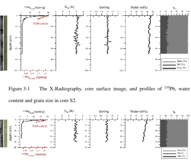
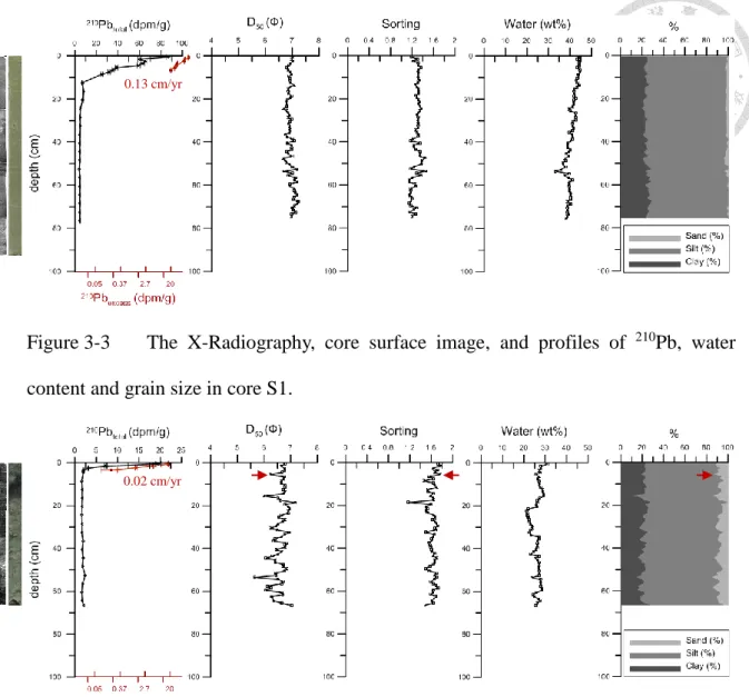
S2, S6, S1 and B4G are located in the intraslope basins on the Gaoping Slope, the GPSC divides them into two symmetric parts, where S2 and S6 are located at west side of the GPSC, while S1 and B4G are situated at the east side of the GPSC. In S2, S6 and B4G cores, the 210Pb activity decreased exponentially with increasing depth, indicating a constant sediment accumulation rate with no significant particle mixing process (Figure 3-1; Figure 3-2; Figure 3-4). In core S1, a small decline in 210Pb activity within the subsurface layer, but for most of the profile it still follows an exponential decay
between fine and very fine silt (most of them falls around 7φ). However, B4G has more variations in the grain size profiles and it can be noted that there’s a decline in the median grain size profile, high sorting value, and an increase in the coarser grain fraction at the depth of 5.5 cm which can indicate an event layer. The sedimentation rates derived from the excess 210Pb in these cores are as follow: S2: 0.06 cm/yr; S6: 0.04 cm/yr; S1: 0.13 cm/yr; B4G: 0.02 cm/yr.
Figure 3-1 The X-Radiography, core surface image, and profiles of 210Pb, water content and grain size in core S2.
Figure 3-2 The X-Radiography, core surface image, and profiles of 210Pb, water content and grain size in core S6.
0.04 cm/yr 0.06 cm/yr