Research Note 01/2010 9 February 2010
WHAT TRIGGERED CHINA’S ECONOMIC SLOWDOWN IN 2008? 1 THE ROLE OF COMMODITY PRICE VOLATILITIES
Prepared by Zhiwei Zhang and Honglin Wang Research Department
Abstract
This note studies what triggered China’s economic slowdown in 2008. We present two findings. First, the slowdown started in July 2008, before the financial crisis in developed economies affected China’s exports, so external demand was not the trigger for the slowdown. Secondly, a case study on China’s steel industry, a key industry that experienced a slowdown during the period, reveals that commodity price shocks played an important role in the boom and bust of the steel industry. We conclude that the 2008 economic slowdown in China was triggered by a commodity price shock rather than by an external demand shock. The external demand shock exacerbated the problem, but it was not the first domino to fall in China.
Authors’ E-Mail Addresses:
[email protected]; [email protected]
1 The authors thank Janet Kong, Dong He, and Lillian Cheung for comments. Daniel Law provided excellent research assistance.
The views and analysis expressed in this note are those of the authors, and do not necessarily represent the views of the Hong Kong Monetary Authority.
I. INTRODUCTION
The Mainland economy slowed substantially in 2008. Why did this happen? According to conventional wisdom, the main reason is the financial crisis in developed economies that led to a decline in demand for China’s exports. But a closer look at the macro data in China indicates that such conventional view might be misleading. The significant slowdown in the Mainland economy began in July 2008, while the financial crisis in the US started to affect the rest of the world in September when the Lehman Brothers collapsed, so the former cannot be the cause of the latter.
This note argues that China’s economic slowdown in July 2008 was caused by a sharp decline in commodity prices. The slowdown was exacerbated by the decline in external demand due to the US financial crisis in September 2008.
While the role of the financial crisis has been well acknowledged, the commodity price shock has been largely neglected in academic research and policy analysis.
We illustrate the role of commodity price shock in China’s slowdown by providing two sets of evidence. First, we compare the performance of export-oriented industries and other industries before and after the US financial crisis in September 2008. If external shock is indeed a key factor behind the slowdown, export-oriented industries would perform worse than other industries.
We find that: (i) from May to August 2008 (before the US financial crisis broke out), both export-oriented industries and other industries slowed down, and there is no correlation between export exposures and the degree of economic deceleration;
(ii) from August to November 2008, export-oriented industries weakened more than other industries. The validity of the above empirical evidence depends critically on the measure of export exposure. Direct exports by individual industries are not the best measure for such exposure as output of a particular industry can be used as intermediate inputs to be exported indirectly by another industry. We utilise the input-output table to capture this indirect export exposure.
Section II provides details on how to construct such a measure.
Secondly, we conduct a case study on the steel industry, which was a key industry in China that experienced a slowdown during the summer of 2008.
The steel industry experienced a dramatic boom in early 2008 and an equally dramatic collapse afterwards. We examine the main sources of demand for steel output, and illustrate that the ups and downs in China’s steel industry was to a large extent driven by the unprecedented volatility in commodity markets. Steel producers in China were attracted by the rapid rise in steel prices in early 2008 and built up iron ore inventories in anticipation of a further rise in prices, only to find the crash in steel and iron ore prices in July 2008 and thus a huge loss incurred.
We illustrate from an industry case study perspective how commodity price shocks affected the steel industry in China. This issue is also related to a small but growing literature on the evolving financialisation of commodities. Tang and Xiong (2009) argue that the correlation between commodity market and equity market rose substantially in recent years as commodity market is increasingly influenced by investors who treat commodities as an asset class. Concerns on commodity price volatilities have appeared in some research reports (for instance, UNCTAD, 2009), but mainstream economists generally do not subscribe to the view that financial forces are behind the high commodity price volatilities (Krugman 2008). Nevertheless, our focus here is not on the cause of the commodity price shocks but on their consequences.
The note is arranged as follows. Section II explores the timing of the slowdown in the Mainland economy relative to the collapse of commodity prices and the outbreak of the financial crisis in the US, and illustrates the differences in the slowdown across industries. Section III conducts a case study on the steel industry to examine the connection between commodity prices and industrial output. Section IV concludes and discusses policy implications for China.
II. THE SLOWDOWN IN 2008:WHAT WAS THE TRIGGER?
Conventional wisdom tends to attribute the slowdown in China to the collapse of Lehman Brothers and the US crisis. A closer look at the production and trade data casts doubt on this claim. As Chart 1 shows, industrial production started to weaken in China from July 2008, but exports started to fall only in October. While the export slowdown exacerbated the economic slump, it was not the trigger.
Chart 1: Industrial production and exports in China
0 2 4 6 8 10 12 14 16 18 20
Feb-08 May-08 Aug-08 Nov-08 Feb-09 May-09 Aug-09
-30 -20 -10 0 10 20 30
Industrial Production Growth, lhs
Export Growth, rhs July
October
%, YoY %, YoY 3MMA
Source: CEIC.
Another way to gauge to what extent the economic slowdown was affected by the deceleration in export growth is to examine correlations between industrial production and export dependence across industries.2 If exports were the main driver of the weakness in industrial production, the output of more export-dependent industries should decrease more compared to those that were less dependent on exports.
It is not straightforward to derive export dependence of an industry because any measure of export dependence based on direct export data could be misleading. This is because the output of an industry can also be used as inputs to other industries which export their products. Therefore, instead of relying on industry-level export data to measure export dependence, we employed the Input-Output (IO) table to calculate actual export dependence for each industry, which includes both the direct exports by each industry and the indirect exports for each industry through its linkages to other industries. For example, the direct exports of the coal mining industry were only 0.95% of total output between January and November 2008, but its actual export dependence was much higher at over 4.5% after taking into account indirect exports by other industries which used coal as important inputs. Details about calculating the indirect export exposure can be found in the Appendix.
2 We focus on the manufacturing industries in this study because of availability and quality of data.
Based on these data, Chart 2 shows two scatter plots on changes in industrial production (IP) and export dependence across industries. The first scatter plot refers to changes in IP from May to August 2008 (before the collapse of Lehman Brothers), while the second refers to changes in IP from September to November 2008. The charts show that, before Lehman’s collapse, there is limited correlation between changes in IP growth and export dependence across industries.
In other words, export dependence does not appear to be a major factor explaining the slowdown at industry level. After Lehman’s collapse more export-dependent industries seemed to suffer slower IP growth, though the correlation is not statistically significant.
Chart 2: Export dependence and changes in growth of industrial production
y = -0.0299x - 2.5761 (0.0723) (1.3204)
-20 -10 0 10 20 30 40 50
0 10 20 30 40 50 60
A ug08 - M ay08 Linear (Aug08 - May08) Change in industrial
production growth, %yoy
Export share (indirect adjusted)
(%)
y = -0.1703x - 2.9834 (0.1288) (2.3535)
-30 -20 -10 0 10 20 30
0 10 20 30 40 50 60
Nov 08 - Aug08 Linear (Nov 08 - A ug08) Cha nge in industr ial
production growth, %yoy
Export share (indirec t adjusted)
(%)
Note: The horizontal axis measures the actual export dependence, after adjusting for indirect exports through upstream-downstream industry linkages. The vertical axis measures the change in annual growth rates of industrial outputs measured in three months. For the chart on the left, the change refers to August 2008 versus May 2008. For the chart on the right, the change refers to November 2008 versus August 2008.
Sources: CEIC and staff estimates.
Could the mismatch in the slowdown in IP and exports be driven by the lag between export orders and export delivery? In other words, could it be that export orders declined in July 2008 which led to slower growth in IP, and exports only weakened later because of the production lag? If this is true, we should observe industries that experienced more decline in export orders to cut down production more. We utilise the Purchasing Managers’ Index (PMI) to measure changes in new export orders at industry level, and construct two scatter plots between changes in IP growth and changes in new export orders (Chart 3). Again, the first scatter plot refers to changes in IP from May to August 2008 (before the collapse of Lehman Brothers), while the second refers to changes in IP from September to November 2008.
Chart 3: New export orders and changes in growth of industrial production
y = 0.0431x - 2.2770 (0.1215) (1.1314)
-15 -10 - 5 0 5 10
-25 -20 -15 -10 -5 0 5 10
Aug08 - May08 Li near (Aug08 - May 08) Change in industrial
production growth, %yoy
Change in new export or der PMI
y = -0.2165x - 7.4734 (0.1954) (4.0003)
-25 -20 -15 -10 -5 0 5 10 15 20 25
-50 -40 -30 -20 -10 0
Nov08 - A ug08 Linear (Nov08 - Aug08) Cha nge in industr ial
production growth, %yoy
C hange in new expor t order PMI
Note: The horizontal axis measures the change in PMI export new order index in two months.
The vertical axis measures the change in annual growth rates of industrial outputs measured in three months. For the chart on the left, the change refers to August 2008 versus May 2008. For the chart on the right, the change refers to November 2008 versus August 2008.
Sources: CEIC and staff estimates.
We find no correlation between changes in export orders and changes in IP growth across industries before the Lehman bankruptcy. After the bankruptcy, the correlation between the two became negative, implying that the decline in export orders was associated with higher IP growth, which is counter-intuitive. We therefore conclude that the time lag between export orders and export delivery was not likely to be the reason for the mismatch between exports and IP growth. In the next subsection, we will go through a case study on the steel industry, a key industry in China that experienced a slowdown during the summer of 2008, to find out what actually caused the decline in steel output.
III. THE SLOWDOWN IN THE STEEL INDUSTRY
The volume of the steel production in China more than tripled in the last 10 years and China has become the largest steel producer in the world, accounting for about 30% of the global output. In value terms, the steel industry accounted for 9.1% of China’s total industrial output in 2008, with about 10% of the steel output shipped overseas (CEIC). The domestic market for steel products is dominated by domestic manufacturers, with the value of steel imports being only 3% of the domestic steel output.
The steel price rollercoaster in 2008
The steel price in China rallied in the first half of 2008 by around 40% and collapsed some time around July 2008 (Chart 4). By November 2008 the steel price reversed all its gains and returned to its 2007 level. China was not the only country that went through the steel price roller coaster. The international steel price doubled in the first half of 2008 and also lost its gains quickly afterwards (Chart 5, left). The surge in international steel price led to a rise in exports in the first half of 2008, and the subsequent price collapse led to a sharp decline in exports (Chart 5, right).
Chart 4: Steel price and steel industry production growth
-10 -5 0 5 10 15 20 25 30
Jan-07 Jul-07 Jan-08 Jul-08 Jan-09
0 20 40 60 80 100 120 140 160
% 180
Steel IP growth, lhs
China's steel price index, rhs
Sources: CEIC and Wind.
Chart 5: Steel prices and exports
50 100 150 200 250 300
Feb-04 Jun-04 Oct-04 Feb-05 Jun-05 Oct-05 Feb-06 Jun-06 Oct-06 Feb-07 Jun-07 Oct-07 Feb-08 Jun-08 Oct-08 Feb-09 Jun-09 50
100 150 200 250 300
China steel price index International steel price index
0 10 20 30 40 50 60 70
Jan-07 Feb-07 Mar-07 Apr-07 May-07 Jun-07 Jul-07 Aug-07 Sep-07 Oct-07 Nov-07 Dec-07 Jan-08 Feb-08 Mar-08 Apr-08 May-08 Jun-08 Jul-08 Aug-08 Sep-08 Oct-08 Nov-08 Dec-08 Jan-09 Feb-09 Mar-09 Apr-09 May-09 Jun-09 0 50 100 150 200 250 300 350
Direct-Export (LHS) International steel price index (RHS) RMB bn
Sources: CEIC and Wind.
Reasons behind the steel price volatility: domestic demand or global demand?
So what caused the steel price to rise so sharply in the first half of 2008 and then to fall so much afterwards? A popular story in the financial press is that the demand dynamics in China drove international prices. But this story does not fit the data. To illustrate this point, we explore the domestic demand for steel by looking at sectoral-level steel consumption. Chart 6 shows the structure of domestic steel usage, which indicates that construction and machinery were the top two steel consumption sectors, and accounted for 54% and 20% of the total domestic steel demand respectively in 2008. Examining the dynamics in these two sectors allows us to verify if domestic demand in China went through the same cycles as steel prices did.
Chart 6: Domestic consumption structure of the steel industry in 2008
construction 54%
machinery 20%
pipeline industry 1%
others 8%
automobile 6%
power industry 4%
shipbuilding 3%
railway 1%
electronics 2%
container industry 1%
Source: Li, 2009.
The demand for real estate is a major determinant of growth in the construction sector. The downturn in the floor space sold in China started in the second half of 2007, which was in line with the collapse of the US housing market (Chart 7). The tightening of China’s monetary policy, which started in the second half of 2007, was an important reason for the downturn in the housing market, and the dynamics between the housing market and monetary policy was similar to the pattern in the US market. It is not hard to infer that the gloomy housing market was not likely to be the main driver of rising prices in the steel market.
Chart 7: Real estate market and steel industry production
-60 -40 -20 0 20 40 60 80
Feb-07 Aug-07 Feb-08 Aug-08 Feb-09 Steel production growth, YoY Floor space sold YoY
%
Sources: CEIC and staff estimates.
The second main source of demand for steel comes from the machinery industry. The machinery industry consists of a number of small subsectors and we selected four main subsectors to represent the machinery industry, namely metal products; universal equipment manufacturing; electric machinery and equipment; and communication, computer and other electronic equipment. In general, the machinery industry did not go through a boom in early 2008, and so it does not appear to explain the rise in steel price; which implies that machinery industry was unlikely the trigger for the increase in steel prices (Chart 8).
Chart 8: Machinery industry and steel industry
-10 -5 0 5 10 15 20 25 30
Feb-07 Apr-07 Jun-07 Aug-07 Oct-07 Dec-07 Feb-08 Apr-08 Jun-08 Aug-08 Oct-08 Dec-08 Feb-09 Apr-09 Jun-09
VAI growth of Steel YOY VAI growth of Metal Products YOY
VAI growth of Universal Equipment Manufacturing YOY
%
-10 -5 0 5 10 15 20 25 30
Feb-07 Apr-07 Jun-07 Aug-07 Oct-07 Dec-07 Feb-08 Apr-08 Jun-08 Aug-08 Oct-08 Dec-08 Feb-09 Apr-09 Jun-09
VAI growth of Steel YOY
VAI growth of Electric Machinery & Equipment YOY
VAI growth of Communication, Computer & Other Electronic Equipment YOY
%
Source: CEIC.
The above analysis indicates that domestic demand did not seem to be the driving force behind the ups and downs of steel prices in China and the international market. An alternative explanation is that domestic prices were driven by international prices. Interestingly, prices of steel, iron ore (main input for steel production), and oil prices all followed similar cycles in 2008 (Chart 9).
A plausible hypothesis therefore is that a common global shock has pushed commodity prices up and down in 2008.
Chart 9: Steel, iron ore, and oil prices
0.5 1 1.5 2 2.5
Jan-07 Jul-07 Jan-08 Jul-08 Jan-09
0.5 1 1.5 2 2.5
Iron ore price International oil price index International steel price index
Sources: CEIC and WIND.
How did the commodity price fluctuations affect steel producers?
The Mainland steel producers suffered huge losses in 2008 because they were misled by the price signals. In the first half of the year, both iron ore and steel prices soared in the international market, which gave two signals to the steel producers: more steel production can lead to more profits even though domestic demand is weak, as the international market would absorb the output; and building up an iron ore inventory is profitable. Consequently, the steel producers continued to build up their inventories and purchased more iron ore from the international market (Chart 10).3 When steel and iron ore prices tumbled after July 2008, it affected the steel manufacturers through two channels. First, the price collapse damaged the balance sheets of steel manufacturers who built up an inventory of iron ore in anticipation of higher prices. Both Mainland and foreign
3 About 70% of the inventory cost came from raw material inventory (Chart 10, Right).
firms had to write down huge losses as they marked their assets to the market value (Chart 11). Secondly, the lower price of steel led to higher uncertainty for prices in the future. Some end-users might have decided to put off their orders as they expected that the price would keep on dropping. The whole steel industry had to go through a “destocking” process – to write down the valuation loss on their iron ore and steel inventory, and stop buying iron ore until their inventory was run down.
This destocking process in turn caused a sharp slowdown in investment demand and the Mainland economy. The recent expansionary monetary policy in China should help firms alleviate the burden caused by inventory loss and bring the economy back on track (Yi, 2009).
Chart 10: Prices and raw material inventory
150 200 250 300 350 400 450 500 550
Jan-07 Mar-07 May-07 Jul-07 Sep-07 Nov-07 Jan-08 Mar-08 May-08 Jul-08 Sep-08 Nov-08 Jan-09 Mar-09 May-09 Jul-09
0.5 0.7 0.9 1.1 1.3 1.5 1.7
Total Inventory (finshed goods+raw materials, LHS) Domestic steel price index (RHS)
RMB bn Jan 2007=100
150 200 250 300 350 400
Jan-07 Mar-07 May-07 Jul-07 Sep-07 Nov-07 Jan-08 Mar-08 May-08 Jul-08 Sep-08 Nov-08 Jan-09 Mar-09 May-09 Jul-09
0.8 1 1.2 1.4 1.6 1.8 2 2.2 2.4
Inventory cost for raw materials (LHS) Iron ore price index (RHS) RMB bn
Source: Wind.
Chart 11: Inventory write-downs for global major steel producers
Inventory Write-dow ns
0 500 1000 1500 2000 2500 3000 3500
ArcelorMittal Nippon Steel
Baosteel Group
Anshan Steel
Wuhan steel
Million US$
2008 2007
Ratio of Inventory Write-downs to sales revenues
0 5 10 15 20 25 30 35
ArcelorMittal Nippon Steel Baosteel Group
Anshan Steel Wuhan steel
%
2008 2007
Sources: Annual reports from firms.
IV. CONCLUSION
This note argues that the 2008 economic slowdown in China was triggered by a commodity price shock rather than by an external demand shock.
The external demand shock exacerbated the problem, but it was not the first domino to fall in China. While this note does not cover any sophisticated statistical analysis, it provides some food for thought by illustrating some stylised facts and proposing alternative hypotheses that are different from conventional wisdom. Given the importance of these issues to the Mainland economy, more research is warranted.
If our hypotheses are correct, it would have important implications for economic policies. The standard economics textbook suggest financial demand in commodity market stabilizes prices, which is not in line with what we experienced in the past several years Conventional wisdom believes that financial demand in the commodity market improves welfare because of its role in price discovery and risk transfer, but again recent experience shows the answer may not be that simple. We look forward to further research in this area.
Appendix: Measuring Export Dependence
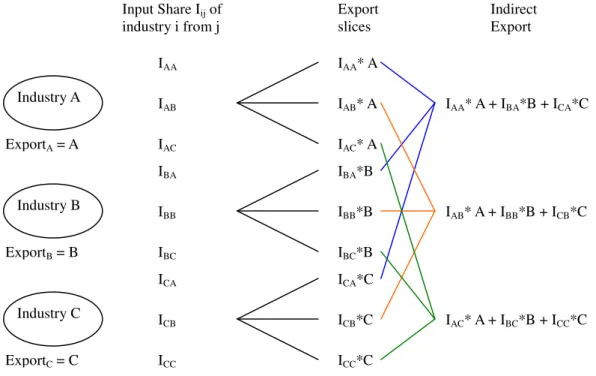
Export dependence is defined as the share of output from a given industry that is exported, also taking into account output used as intermediate inputs that are to be exported indirectly by other industries. To estimate the indirect export exposure, exports are adjusted according to contributions to each industry in a customized Input-Output (IO) table. The IO table contains 39 sectors, showing the inputs of each industry from other industries in 2002. For each industry, the input shares of the 39 industries are tabulated. Since some output of an industry is the input of another, the exports of a particular industry are distributed across industries which provide its inputs. More specifically, the direct exports of an industry are divided into 39 slices, with values proportional to inputs from the 39 industries. Therefore, if industry A provides more (less) inputs to industry B, it will receive more (less) exports from industry B. By aggregating the slices received from all industries, the exports adjusted for indirect exposure of an industry can be obtained. An example of a 3-sector economy is shown in Figure 1.
On the other hand, the total production in each industry is the total revenue of the industrial enterprises. Since some revenue is made from selling output which becomes input of other domestic industries, export dependence, which is adjusted export divided by total revenue, should reflect the true importance of exports towards each industry.
Figure 1: Example of adjusting indirect export for a 3-sector economy
Industry A
Industry B
Industry C ExportA = A
ExportB = B
ExportC = C
IAA
IAC
IAB
IBA
IBC
IBB
ICA
ICC
ICB
Input Share Iij of industry i from j
IAA* A
IAC* A IAB* A
IBA*B
IBC*B IBB*B
ICA*C
ICC*C ICB*C Export slices
Indirect Export
IAA* A + IBA*B + ICA*C
IAB* A + IBB*B + ICB*C
IAC* A + IBC*B + ICC*C
REFERENCES
Krugman, Paul, 19 March 2008, “Commodity Prices (wonkish)”, The New York Times.
Li, Chuangxin, 2009 “The Consumption Structure of China’s Steel Industry”, http://www.custeel.com.
Tang, Ke and Xiong, Wei, 2009, “Index Investing and the Financialization of Commodities”, Princeton University working paper.
UNCTAD, 2009, “Trade and Development Report, Chapter II: The Financialization of Commodity Markets”, UNCTAD/TDR/2009.
Yi, Gang, 2009, “The People’s Bank of China Improves Credit Structure via Five Measures”, Xinhua News (2009-4-22).