分析不同變異考量下之簡化模型對排序佳化的影響：以迴流產線產能分配為例

國立臺灣大學電機資訊學院電機工程學系 碩士論文

Graduate Institute of Electrical Engineering

College of Electrical Engineering and Computer Science National Taiwan University

Master Thesis

分析不同變異考量下之簡化模型對排序佳化的影響：

以迴流產線產能分配為例

Analysis of How Selecting Simplified Models of Different Variability Affects Ranking for Ordinal Optimization: Re-entrant Line Capacity Allocation Case

張鈞閔

Chun-Ming Chang

指導教授：張時中、陳俊宏 博士

Advisor: Shi-Chung Chang, Chun-Hung Chen Ph.D.

中華民國 104 年 8 月

August 2015

誌謝

首先要感謝台大電機系所這六年來的栽培，特別感謝我的指導教授張時中博 士在兩年研究期間耐心指導我做研究的方法，叮囑我們要有左右互搏的思辨精神，

您對研究的嚴謹態度對我影響重大，使本論文得以順利完成。特別感謝指導教授 陳俊宏博士，每次討論後都覺得豁然開朗、如沐春風，您總能給予精闢的建議，

能和您做研究是我莫大的榮幸。謝謝兩位指導教授作為研究路上堅實的巨人的肩 膀。本論文由國科會計畫(編號 NSC 102-2221-E-002-206, 102-2219-E-002-012, 103-2221-E-002-220-MY2) 的部分支持下完成，特此致謝。

在此更要感謝學位考試委員台灣大學張時中教授、美國喬治梅森大學陳俊宏 教授、美國康乃狄克大學陸寶森教授給予本論文的指正與建議，讓本論文更臻完 整。特別感謝美國康乃狄克大學陸寶森教授在擔任訪問學者期間給予我研究上的 寶貴意見，與您討論總是獲益良多，謝謝您使得本論文的格局與面向更加寬廣。

謝謝 Lab 207 的學長姐與同學們，謝謝輝哥，身兼實驗室助理幫忙我們處理 很多行政事務；謝謝舜丞是我研究生涯最好的榜樣，我會努力向你看齊；謝謝在 實驗室共同奮戰的泓捷、名傑、家興、振豪、羅賓、琳茵、冠霖、惠平、登傑。

我會記得這些日子一起度過的漫漫長夜和一同散步閒話的小確幸。泓捷總保持正 面的態度，謝謝最後這段時間的陪伴與鼓勵；名傑很務實的做好每件事情，相信 一定會結出很美好的果實；健談的羅賓希望 Lab 207 是你很好的回憶；坐在我旁 邊一年義氣的家興，陪我玩耍、吃飯、睡覺；振豪，要記得我的李星，給酷；琳 茵、冠霖、惠平、登傑，祝你們研究順利。最後想要特別謝謝小高這兩年來不僅 在研究的教導，在生活中跟你分享事情總能得到很多收穫，祝你之後一切順利。

最要感謝我的家人們，謝謝辛苦工作的父親、母親提供我一個安心無虞的環 境，謝謝哥哥時常的關心與照顧，謝謝女友抒珉一直是我重要的依靠。謝謝你們 像大海般的溫柔與包容，讓我懷抱遠大志向勇往直前。紙短情長，謝謝你們無私 的奉獻與栽培造就今天的我。謹以此論文，獻給所有陪伴我、幫助我的人。

I

Abstract

Ordinal optimization (OO) focuses on “ranking” in performances among designs instead of their “values” and exploits a goal softening strategy aiming at “good enough” designs with high probability as opposed to an optimal design for sure.

Ordinal transformation (OT) is an OO technique that utilizes a simplified model for perform evaluation and ranking to further reduce computational effort. There are often multiple choices of simplified models for a system that capture different levels of details or aspects. The selection of an appropriate simplified model is a key factor for the effectiveness of OT and OO. Thus, how to select simplified models for ranking and how to analyze the goodness of simplified models are significant and challenging problems for OT and OO.

However, there is little literature to theoretically explore the influences of different simplified models on ranking largely because the comparison among various simplified models is often difficult in lack of a common ground. In addition, ranking is a relative index instead of an absolute index. The goodness of ranking is not straight forward to quantify let alone to analyze.

In this thesis, machine capacity allocation for re-entrant lines, an important engineering optimization problem, is adopted as the conveyor problem to investigate the selection of an appropriate simplified model. In particular, Jackson network approximation (JNA) and queueing network analyzer (QNA), two commonly used queueing network approximation models, are studied with the mean cycle time as the performance index. Both models are developed based on parametric decomposition, but JNA has unity SCVs due to its exponential time assumptions while QNA has heterogeneous SCVs. Thus, we compare between QNA and JNA to investigate how

II

selecting simplified models of different variability affects ranking and analyze the goodness of a simplified model with consideration of heterogeneous SCVs.

A key step in the investigation is the quantification of the goodness of rankings by simplified models. This is difficult since “ranking” is a relative index, not an absolute index. A bound and ranking analysis (BRA) is innovatively developed to quantify and analyze the goodness of rankings by simplified models. BRA consists of two innovations:

i) Analyze the upper and lower bounds of simplified models,

ii) Derive the probability of correct ranking under the assumption of actual cycle time being uniformly distributed between its upper and lower bounds.

The probability of correct ranking between a pair of designs for a single GI/G/m queue is first studied. With the variation of two QNA approximations, the least variation of their upper bound is derived and this helps obtain a higher probability of correct ranking α.

The results and insights from BRA are as follow.

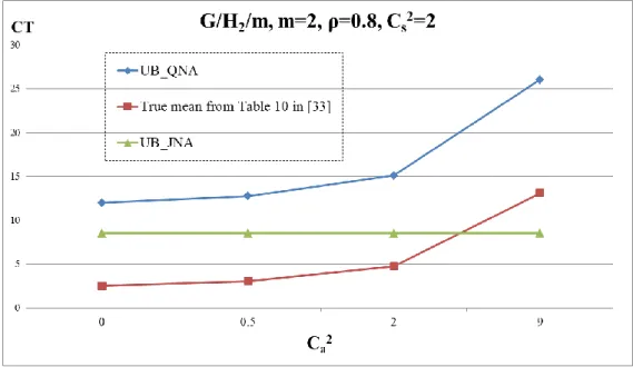
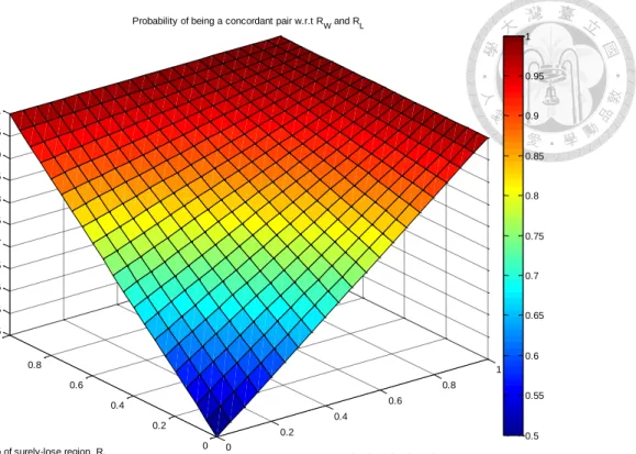
i) Showed that QNA approximation is bounded by known upper and lower bounds proposed by Kingman, Brumelle and Marshall respectively.

ii) Compared with existing literature results, QNA captures the variations of true expected cycle time well because of heterogeneous SCVs but JNA does not.

iii) Obtained a valuable insight from derived α that capturing heterogeneous SCVs benefits the ranking of top designs and improves probability of correct ranking because variability has greater impacts on cycle time while lower utilization.

Based on the above for a single GI/G/m queue, BRA is then extended to general re-entrant lines with multiple workstations. Rank correlation, which measures the concordance of pair-wise comparisons in two quantitative indices, is adopted to quantify the goodness of ranking.

III

Simulation studies over a five-station re-entrant line demonstrated that rank correlation of QNA always outperforms that of JNA, and the difference is especially significant for top designs. This is consistent with the insight iii) obtained from BRA.

Then, in order to investigate the effects of heterogeneous SCVs, the original design space is transformed using true ranking, and in this ordinal space each thirty designs are clustered into a group. After grouping, we found that heterogeneous SCVs contribute to improve differentiation between groups and also make designs in a group better separated, which benefit raise the probability of correct ranking. This is why heterogeneous SCVs benefit rank correlation of a simplified model.

In summary, the contributions of this thesis are as follows.

i) Adopted re-entrant line capacity allocation as the conveyor problem to meaningfully compare two simplified models: JNA has unity SCVs while QNA has heterogeneous SCVs,

ii) Established theoretical foundations, BRA, to analyze the probability of correct ranking and quantify the goodness of different simplified models,

iii) Derived the probability of correct ranking between a pair of designs α, and a valuable insight is that heterogeneous SCVs have greater impacts on top designs, iv) Simulation studies demonstrated that heterogeneous SCVs contribute to improve

differentiation between groups and make designs in a group better separated, v) Because of iv), QNA always outperforms JNA in terms of rank correlation, and

the difference is especially significant for top designs. It is consistent with iii), vi) Investigate in aspects of both theory and experiment how selecting simplified

models of different variability affects ranking for OO and OT.

Keyword: Model selection, ordinal optimization, heterogeneous variability, ranking

analysis, re-entrant line capacity allocation

IV

中文摘要

排序佳化(OO)著重在設計間績效值的排名而不是績效值本身，並利用目標軟 化的策略以很高機率找到足夠好的設計取代勢必求得最佳設計。排序轉換（OT）

是一排序佳化的技術，其利用一個簡化模型的績效評估和排名進一步地減少計算 量。在同一個系統中經常有多個簡化模型的選擇，其掌握到系統中不同細節或不 同面向。選擇一個適合的簡化模型決定 OT 和 OO 效能的關鍵因素，因此如何選 擇用來排名的簡化模型以及如何分析簡化模型的優劣，對於 OT 和 OO 來說都是 重要且挑戰的問題。

因為不同簡化模型之間大多缺乏一個共同的依據，使得不同的簡化模型之間 的比較是非常困難，以致於鮮少有文獻從理論上探討不同簡化模型對於排名的影 響。此外，因為排名是一個相對指標而非絕對指標，使得簡化模型的排名之優劣 難以直接量化更遑論分析。

在本論文中，我們選用一個重要的工程優化問題─迴流產線產能分配作為載 具以研究如何選擇適合的簡化模型。採用傑克遜網絡近似（JNA）和排隊網絡分 析儀（QNA）這兩種常見的排隊網絡近似模型進行研究，並以其平均生產週期 時間為績效指標。此兩種模型皆發展自參數分解法，但 JNA 由於指數分配的假 設為統一的 SCVs 而 QNA 則有異質的 SCVs。 因此我們對 QNA 與 JNA 進行比 較來研究如何考量不同變異的簡化模型選擇對排名的影響，並分析考量異質 SCVs 的簡化模型之優劣。

本研究其中一個關鍵在於量化簡化模型的排名之優劣，因為排名是一個相對 的指標而不是絕對指標導致此量化的困難。為此，我們創新地開發了一界限與排 名分析(BRA)，用來量化和分析簡化模型的排名之優劣。BRA 有兩項創新之處:

i) 分析簡化模型的上限與下限

ii) 推導正確排序機率，假設真實生產週期在其上、下限間為均勻分佈

V

首先分析在單一 GI/G/m queue 中正確排序一對設計的機率，從兩個設計間 QNA

近似績效值變化量推導其上限的最少變化量，因而得到更好的正確排序機率 α。

從 BRA 的分析可得到下列結果與觀察:

i) 證明 QNA 近似績效值落於分別由 Kingman、Brumelle 和 Marchall 所提出

的上限與下限,

ii) 與文獻中的結果比較發現，QNA 因為掌握到異質 SCVs 的特徵，故能掌

握到真實的期望生產週期之變化，但 JNA 不行

iii) 從 α 可得知一重要的觀察─因變異對於生產週期的影響在產線於低使用

率時特別顯著，所以異質 SCVs 對前若干名設計的影響較大因而有助於提 高正確排序機率。

根據上方對單一 GI/G/m queue 的分析結果，將 B＆R 分析推展到普遍常見的有多 工作站之迴流產線。以排名相關性(rank correlation)作為量化其排名優劣的指標，

排名相關性是用來衡量兩個定量指標間成對比較是否一致的統計值。

從實驗模擬發現 QNA 的排名相關性總優於 JNA 的排名相關性，兩者差異在 前若干名設計中特別顯著，此結果與 BRA 得到的 iii)觀察一致。為了更加瞭解異 質 SCVs 的效果，我們將原本的設計空間依據設計的真實排名轉換到一排序空間，

在該排序空間中的每三十個設計都群聚成一組。分組後我們發現異質 SCVs 有助 於增加各組間的差異且使得同組內之設計被更好地區隔，這兩者都有助於提升正 確排序機率─這就是為什麼考量異質 SCVs 能增進排名相關性。

總結本論文貢獻在於，

i) 以迴流產線產能分配問題為載具比較兩種基於相同理論基礎的簡化模型，

有統一 SCVs 的 JNA 和異質 SCVs 的 QNA

ii) 建立 BRA 來分析正確排序機率以此作為量化簡化模型之優劣的依據

iii) 推導正確排序機率α，和一重要觀察─異質 SCVs 對於前若干名設計有較

大的影響

iv) 模擬結果顯示異質 SCVs 有助於增加各組間的差異且使得同組內之設計被

VI

更好地區隔

v) 因為 iv)的結果，QNA 在排名相關性上總優於 JNA，且兩者差距在前若干

名設計中尤其顯著，和 iii)的結論一致。

vi) 從學理和實驗的面向分析不同變異考量下之簡化模型對排序佳化和排序

轉換的影響

關鍵字: 模型選擇、排序佳化、異質變異、排名分析、迴流產線產能分配

VII

Contents

Abstract ... I

中文摘要... IV

Contents ... VII List of Figures ... IX List of Tables ... X

Chapter 1 Introduction ... 1

1.1 Motivation ... 1

1.2 Literature Survey ... 3

1.2.1 Optimal Capacity Allocation of Re-entrant Lines ... 4

1.2.2 Performance Evaluation Models ... 6

1.2.3 Selection of Simplified Models for OO ... 8

1.3 Scope of Research ... 10

1.4 Thesis Organization ... 15

Chapter 2 Conveyor Problem: Re-entrant Line Capacity Allocation ... 16

2.1 Problem Description and Complexity Analysis ... 16

2.2 Mathematical Abstraction of Machine Allocation Problem... 18

2.2.1 Open Queuing Network Modeling ... 18

2.2.2 Formulation: Nonlinear Integer Programming ... 20

2.3 Conveyor Problem for Ordinal Optimization ... 21

Chapter 3 Parametric Decomposition Method for OQN ... 22

3.1 Introduction ... 22

3.2 Class Aggregation ... 24

3.3 Parametric Decomposition Method ... 26

3.3.1 Markovian Routing ... 28

3.3.2 Deterministic Routing ... 29

3.4 Performance Measures ... 31

3.4.1 Node Level Measures ... 31

3.4.2 System Level Measures ... 32

3.5 Two Simplified Models for Re-entrant Line: QNA and JNA ... 33

VIII

Chapter 4 Ordinal Transformation and BRA ... 35

4.1 Ordinal Transformation ... 35

4.1.1 Ranking in terms of Approximations by Simplified Model... 37

4.1.2 Transformation to Ordinal Space ... 40

4.1.3 Performance Index: Rank Correlation ... 40

4.2 BRA of QNA and JNA in single GI/G/m queue ... 42

4.2.1 Bound Analysis of QNA and JNA ... 43

4.2.2 Ranking Analysis of QNA and JNA ... 50

4.3 Summary ... 62

Chapter 5 Extensions of BRA to General Re-entrant Lines ... 64

5.1 BRA of QNA and JNA for General Re-entrant Lines ... 64

5.2 Extension to N Designs ... 71

5.3 Discussion of Variability ... 72

5.4 Summary ... 76

Chapter 6 Machine Capacity Allocation Experiments ... 78

6.1 Overview ... 79

6.2 Selection of Top Designs in Ordinal Space ... 80

6.3 Re-entrant Network Models and Experiment Factors ... 82

6.3.1 Simulation model: 5-station and 2-product model... 82

6.3.2 Experiment Factors ... 86

6.4 Numerical Results ... 88

6.5 Efficiency of Using Simplified Models for OT ... 95

Chapter 7 Conclusions ... 97

Appendix Ranking Analysis of QNA as Simplified Model in Other Cases ... 99

References ... 101

IX

List of Figures

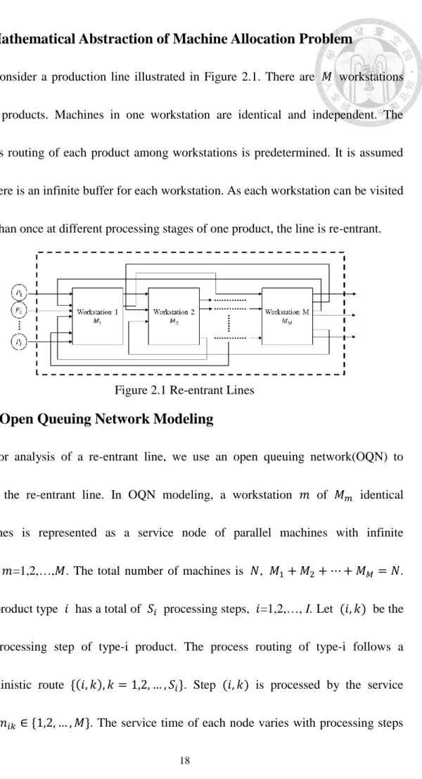
Figure 2.1 Re-entrant Lines ... 18

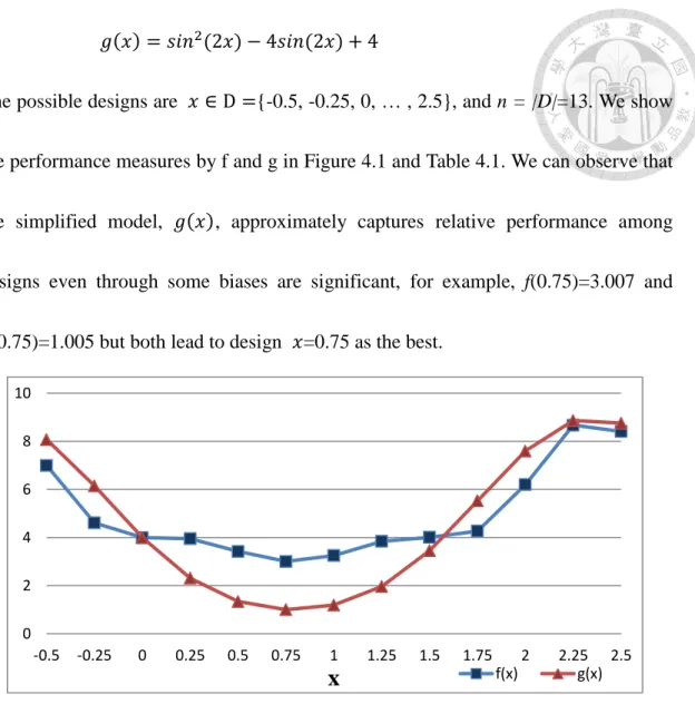
Figure 4.1 An illustrative example of OT ... 39

Figure 4.2 Transformation to ordinal space ... 40

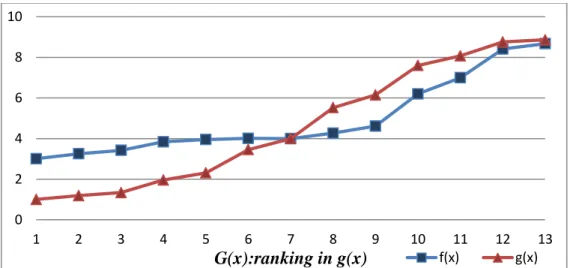
Figure 4.3 Comparison of upper bound between QNA and JNA while SCVs≦1 ... 48

Figure 4.4 Comparison of upper bound between QNA and JNA while SCVs>1 ... 48

Figure 4.5 Advantage of QNA bounds with heterogeneous SCVs ... 49

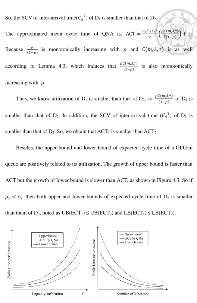
Figure 4.6 UB, ACT, LB w.r.t. utilization and number of machines ... 53

Figure 4.7 Two simple diagrams ... 54

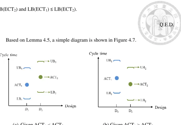
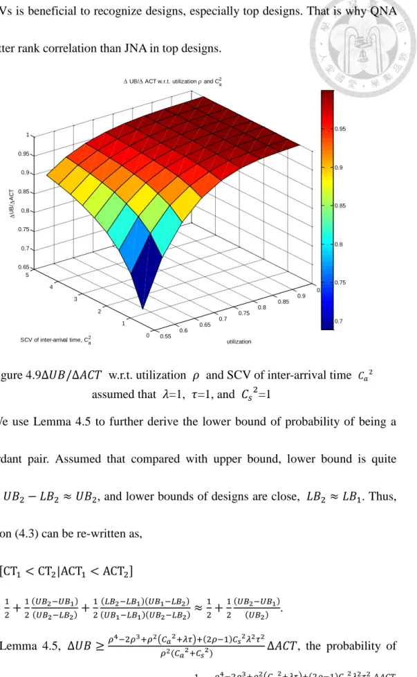
Figure 4.8 Probability of being a concordant pair w.r.t. R

_W

and R

_L

... 58

Figure 4.9∆𝑼𝑩/∆𝑨𝑪𝑻 w.r.t. utilization and SCV of inter-arrival time ... 61

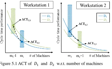
Figure 5.1 CT of

𝑫𝟏 and 𝑫𝟐 w.r.t. number of machines ... 65

Figure 5.2 Four possible cases of bounds given ACT

₁

< ACT

₂

... 66

Figure 5.3 Actual p.d.f. and the p.d.f under our assumption ... 71

Figure 5.4 D

₁

and D

₂

are similar, (a) JNA (b) QNA ... 74

Figure 5.5 D

₁

and D

₂

have distinct differences, (a) JNA (b) QNA ... 76

Figure 6.1 Flowchart of Experiment ... 80

Figure 6.2 A five-workstation and two-product re-entrant Line ... 83

Figure 6.3 Routing of each product ... 83

Figure 6.4 Unstable designs labeled in both Simulation and QNA(JNA) ... 89

Figure 6.5 Performances of DES simulation in original design space ... 90

Figure 6.6 Performances of DES Simulation after OT by QNA ... 91

Figure 6.7 Performances of DES Simulation after OT by JNA ... 91

Figure 6.8 Comparison between QNA and JNA in rank correlation of top-K designs ... 93

Figure 6.9 Grouping after ordinal transformation using true performance ... 94

Figure 6.10 Difference of mean between K

^th

and K+1

^th

group ... 94

Figure 6.11 Coefficient of variance of each group ... 94

X

List of Tables

Table 4.1 Ranking order among designs of this example ... 39

Table 6.1 Release of each product ... 84

Table 6.2 Workstation failure setting ... 84

Table 6.3 Processing steps of each product ... 85

Table 6.4 True rankings of the selected top-10 designs in QNA and JNA ... 92

Table 6.5 Comparison of computation time between QNA and JNA ... 95

1

Chapter 1 Introduction

1.1 Motivation

Ordinal optimization (OO) focuses on “ranking” in performances among designs instead of their “values” and exploits a goal softening strategy aiming at “good enough” designs with high probability as opposed to an optimal design for sure.

Ordinal transformation (OT) proposed by Xu and Chen et al. [1] is an OO technique that utilizes a simplified model for perform evaluation and ranking to further reduce computational effort. Huang et al. [38] proposes an OT approach to transform the original design space into a new one-dimensional space where all designs are positioned according to their ordinal ranks using the simplified model. The original design space may be high-dimensional, have multiple local optimums spread far apart, and include a mix of integer-valued and categorical variables [38]. After OT, the new design space is one-dimensional, likely to be well-behaved and have some global trends [44]. Therefore, OT has the following important advantages: 1) handles a mix of discrete and categorical decision variables in a high-dimensional design space; 2) OT is a general approach and has the potential to effectively perform optimization when simplified models are appropriate.

2

However, there are often multiple choices of simplified models for a system that capture different levels of details or aspects. The selection of an appropriate simplified model is a key factor for the effectiveness of OT and OO. Thus, the selection of simplified models is a significant problem for OT. There are few theoretical results on the effects of rankings by different simplified models for OO since it is difficult to meaningfully compare among different simplification methods in a common ground.

Another challenge of selecting simplified models for OO is the quantification of the goodness of rankings by simplified models. This is difficult because “ranking” is a relative index while “value” is an absolute index. Thus, how to theoretically analyze the goodness of rankings by different simplified models is another challenging problem for OO.

In this thesis, we adopt re-entrant line machine capacity allocation problem as the conveyor problem to investigate selection of simplified models for OO. In a semiconductor fab, there are several products flow through a sequence of processing steps. The production flow of each product consist of a sequence of processing steps , where the flow visits some workstations more than once at different steps of processing. This re-entrant characteristic poses a unique challenge to capacity allocation, since jobs of different products as well as jobs of the same product but at

3

different processing steps may compete for the finite capacity of a workstation.

In the literature, because capacity allocation is crucially significant to semiconductor fab, there has been much research on this problem. Chang et al. [45]

designed a daily target setting system, which helps allocate the capacity to product as well as stages under master production schedule in a horizon of one day. Field applications demonstrated that this allocation method leads to over 20% increase in daily moves and more than 8% decrease of wafers-in-process (WIPs) of a foundry fab case [45]. Therefore, in this thesis, we shall consider the optimal machine capacity allocation for re-entrant lines, an important engineering optimization problem, as the conveyor problem to investigate the selection of an appropriate simplified model.

1.2 Literature Survey

Re-entrant line capacity allocation is regarded as the conveyor problem in this thesis. The determination of number of machines allocated in each workstation of an arbitrary queueing network is a complex problem. There is a mount of literature for the optimal allocation of machines for single node, exponential service and infinite buffer queueing networks, yet not as much literature exists for the case when there are complex topologies like re-entrant lines and general inter-arrival or service time distributions in the network because of the intractability to acquire the exact

4

performance. Such a complex production line can be modeled as an open queueing network [2][3][4][26]. For open queueing networks, parametric decomposition method is a widely used approximation, but it has different characterization on variability terms owing to various assumptions. Therefore, we analyze how the characterization of variability in simplified models affects ranking using re-entrant line capacity allocation as the conveyor problem to investigate the model selection problem for OO and how to analyze the goodness of ranking by simplified models.

Therefore, we review the related works of optimal machine allocation problem in re-entrant lines, and the commonly used techniques and models which developed for performance evaluation of a queueing network.

1.2.1 Optimal Capacity Allocation of Re-entrant Lines

For closed queueing networks, Shanthikumar and Yao [31] formulate the machine allocation problems as a nonlinear integer program and propose a greedy heuristic to maximize throughput.

Dallery and Stecke [32] define the optimal configuration problem in a closed queueing network. Then, use designed decomposition method to determine the best configuration of each subnetwork that yields the highest throughput for the overall closed queueing network, where the number of stations, the number of machines, and

5

the workload allocated to each station defines a configuration of each subnetwork.

Bitran and Tirupati [33] propose a greedy heuristic solution approach to minimize the work-in-process (WIP), instead of using conventional convex programming method. An extension of Bitran and Tirupati formulation is presented by Boxma et al.

[15], which propose a greedy algorithm for machine allocation problem in

multi-server open queueing network with exponential inter-arrival and service processes in order to minimize cost of machine allocation but generate undominated solutions. Later, Frenk et al. [34] propose an improved version of the greedy algorithm proposed by Boxma et al. [15].

Connors et al. [4] develop an open queueing network model for performance evaluation of manufacturing systems characterized by the effect of rework and scrap.

A marginal allocation procedure to determine the number of tools needed to achieve a target cycle time is designed based on the performance estimates form the queueing network models.

Bispo and Tayur

[35] use simulation-based optimization approach and

develop expressions for and validate the appropriate Infinitesimal Perturbation Analysis (IPA) derivatives. These derivatives can be used to determine the optimal parameters of managing re-entrant flow lines.

6

1.2.2 Performance Evaluation Models

We briefly classify the evaluation models as follows: (1) Exact analysis (2) Approximation models (3) Discrete event system simulation.

Exact Analysis

Exact solutions are known by Jackson[5] for open queueing networks with exponential inter-arrival and service time distributions, and probabilistic job routing which described by a routing matrix. The main result is that the solutions have a product form for the stationary multi-dimensional state probability where each product term is the solution of isolated queueing workstations. Kelly[6] extended Jackson’s result to networks with more general routings, i.e. deterministic routing, but inter-arrival and service time distributions still follow exponential distributions.

Gordon and Newell [7], and Baskett et al. [8] extend the result to closed and mixed queueing networks, respectively.

Approximation methods

The lack of success in obtaining exact solutions for general queueing networks has motivated researchers to develop approximation models to evaluate network performances. There are several known approaches, i.e. diffusion approximation [2][10], mean value analysis[3][12], and parametric decomposition methods [3] [10]

[13][14] [15] [16] [17]. Here, we emphasize on parametric decomposition methods.

7

The decomposition method can be roughly described in three basic steps:

Step 1: Analysis of interaction between workstations.

Step 2: Evaluation of performance measure at each station.

Step 3: Evaluation of performance measure for the whole network.

It is well-known that AT&T Bell Laboratories uses the parametric decomposition methods as the basis of their Queueing Network Analyzer (QNA) software package [13] [14]. QNA describes open queueing network with non-exponential service time, non-Poisson arrival processes, and non-Markovian routing, for which exact analytical techniques are unavailable. Bitran and Tirupati [3] improve the parametric approximation. Segal and Whitt [14] proposed the refined approximation model for re-entrant lines with deterministic routing of products. Conner et al. [4] develop an open queueing network model for performance analysis of semiconductor manufacturing.

DES Simulation

Currently, the rapid advances in computing power and memory have opened up the opportunities of optimizing by simulation models, which usually called simulation-based optimization. For those complex systems that are intractable to traditional analytical methods, simulation has often been adopted as an evaluation model because it has the advantage of high fidelity and modeling flexibility in coping

8

with the various system configurations. Examples include the optimization of flow production lines via running a simulation model to find the optimal solution [18] [19].

However, fidelity and flexibility often come with expensive computational cost.

Besides, with the stochastic nature of systems, hundreds of Monte Carlo simulation runs are required to reach a statistically significant evaluation.

1.2.3 Selection of Simplified Models for OO

First, simplification is important because it is central to the model selection process. An approach to modelling that is usually suggested to start by building a simple model and then gradually adding details [20], but starting with a simple model implies there are many initial simplifications in the developer’s mind. The subsequent process of adding details is the inverse of simplification. Brook et al. [23] studied the simplification in the simulation of manufacturing systems and used an alternative approach to modelling is to start by building a complex model and then try to simplify it. Brook pointed out the advantage of this approach is able to examine model’s behavior and indicate which features of the model are important and which are unimportant, and hence the best simplification to perform. Moreover, Johnson et al.

[21] develop a procedure for simplifying a detailed model into a fast simulation model that achieves a statistically in distinguishable level of accuracy and precision.

9

Most of works discuss the accuracy and precision of simplified models in aspect of “value”, and focus on finding a fast enough simplified model even though with

endurable biases. But there are few theoretical results discuss in view of relative

“orders” provided by simplified models. However, for OO the correlation of ranking

among designs by simplified models is much more important than the accuracy of performance of designs.

Xu et al [1] propose an ordinal transformation (OT) framework, which utilizes a simplified model to rank all designs in terms of their approximated performance and then transform the original design space to an ordinal space. There is an illustrative machine allocation example of the OT framework in [1] which uses Jackson network approximation, a model being unity SCVs, as the simplified model of a re-entrant line.

However, Kao et al. [24] study the daily target setting and machine allocation problem and [25] investigate the effects of target-induced variability on cycle time performance, these show the significance of variability for cycle time and also expose the deficiency of the model being unity SCVs. Based on the work of Hu [26], it uses queueing network analyzer, a model being heterogeneous SCVs, as the simplified model of a re-entrant line to quickly translate production goals into production flow control parameters.

Importantly, both [21] and [23] pointed out the phrase of ‘complexity’ or ‘level of

10

detail’ has not been well-defined, and there are no solid foundations in theory to simplify a system, let alone the theoretical comparisons between different simplifications. Based on the previous works, in this thesis we investigate the model selection problem for OO by the comparison of two simplified models: one is unity SCVs and the other is heterogeneous SCVs. Also, we establish the theoretical analysis of how different variability in simplified models affects ranking and demonstrate the validity of using ranking information in OO by an illustrative experiment.

1.3 Scope of Research

Ordinal optimization (OO) focuses on “ranking” in performances among designs instead of their “values” and exploits a goal softening strategy aiming at “good

enough” designs with high probability as opposed to an optimal design for sure.

Ordinal transformation (OT) proposed by Xu et al. [1] is an OO technique that utilizes a simplified model for perform evaluation and ranking to further reduce computational effort. There are often multiple choices of simplified models for a system that capture different levels of details or aspects. The selection of an appropriate simplified model is a key factor for the effectiveness of OT and OO. Thus, how to select simplified models for ranking and how to analyze the goodness of simplified models are significant and challenging problems for OT and OO.

11

However, there is little literature to theoretically explore the influences of different simplified models on ranking, since the comparison among various simplified models, however, is often difficult in lack of a common ground. Moreover, because ranking is a relative index instead of an absolute index, the goodness of ranking by a simplified model is also difficult to quantify let alone to analyze.

In this thesis, machine capacity allocation for re-entrant lines, an important engineering optimization problem, is adopted as the conveyor problem to investigate the selection of an appropriate simplified model. For re-entrant lines, queueing networks are commonly used as approximation models, including Jackson network approximation (JNA) and queueing network analyzer (QNA). Both of them are obtained on the same theoretical basis of parametric decomposition method.

Parametric decomposition method is a widely used approximation model. It decomposes a queueing network into individual network nodes and use first order and second order parameters, mean and variance, to characterize the stochastic arrival and service processes of each node. Owing to various assumptions of networks, parametric decomposition method has different characterization on variability terms.

Xu and Chen et al. [1] use Jackson network as an approximation model of a re-entrant line where assumes the arrival and service processes of each station are all exponentially distributed, a model being unity SCVs. However, [24] shows the

12

significance of considered variability into cycle time performance and also exposes the deficiency of the model being unity SCVs. Based on the work of Hu [26], it uses queueing network analyzer (QNA), a model being heterogeneous SCVs, as the simplified model of a re-entrant line to quickly translate production goals into production flow control parameters.

Thus, we compare between two simplified models, one being unity SCVs (JNA) and the other being heterogeneous SCVs (QNA), to research how different variability in simplified models affects ranking for OO. It is a meaningful comparison because both these simplified models are developed in the same theoretical basis, and the only difference is the characterization of variability.

A key step in the investigation is the quantification of the goodness of rankings by simplified models. A bound and ranking analysis, BRA, is developed to quantify and analyze the goodness of rankings by simplified models. There are two innovations in BRA: 1) Analyze the upper and lower bounds of simplified models; 2) Derive the probability of correct ranking under the assumption of actual cycle time being uniformly distributed between its upper and lower bounds.

The probability of correct ranking between a pair of designs for a single GI/G/m queue is first studied. With the variation of two QNA approximations, the least variation of their upper bound is derived and this helps obtain a higher probability of

13

correct ranking α.

In this case, the results and insights from BRA are as follow.

iv) Showed that QNA approximation is bounded by known upper and lower bounds proposed by Kingman, Brumelle and Marshall respectively.

v) Compared with existing literature results, QNA captures the variations of true expected cycle time well because of heterogeneous SCVs but JNA does not.

vi) Obtained a valuable insight from derived α that capturing heterogeneous SCVs benefits the ranking of top designs and improves probability of correct ranking because variability has greater impacts on cycle time while lower utilization.

Based on the above for a single GI/G/m queue, BRA is then extended to general re-entrant lines with multiple workstations. Rank correlation, which measures the concordance of pair-wise comparisons in two quantitative indices, is adopted to quantify the goodness of ranking. In our experiment, α is greater than 0.75 and significantly difference with the probability of 0.5 like tossing a coin.

Finally, a simulation experiment is conducted over a five-station re-entrant line.

Simulation results show that rank correlation of QNA always outperforms that of JNA and their difference is especially significant for top designs. This corresponds to the insight obtained from our BRA and discussion about heterogeneous SCVs.

Furthermore, we innovatively reverse the logic of ordinal transformation and use true

14

performance as the ranking index, and then cluster each thirty designs to a group.

After grouping, we found that heterogeneous SCVs benefit better differentiation between groups and also make designs in a group better separated. That is why considering heterogeneous SCVs in simplified models improve the rank correlation.

In this thesis, we investigated in aspects of both theory and experiment how selecting simplified models of different variability affects ranking by using re-entrant line capacity allocation as the conveyor problem to compare two simplified models in the same theoretical basis. Finally, we developed the BRA and established theoretical foundations to quantify and analyze the goodness of ranking by simplified models.

The contributions of this thesis are as follows.

1. Adopted re-entrant line capacity allocation as the conveyor problem to meaningfully compare simplified models with different level of details, QNA being heterogeneous SCVs and JNA being unity SCVs,

2. Established theoretical foundation to quantify and analyze how selecting simplified models of different variability affects ranking,

3. Derived a lower bound of probability of correct ranking α in the case of single GI/G/m queue with two designs, and the property of α showed that heterogeneous SCVs have greater impacts on top designs,

4. Simulation study demonstrated that heterogeneous SCVs contribute to improve

15

differentiation between groups and make designs in a group better separated, 5. Simulation result also showed that QNA always outperforms JNA in terms of

rank correlation, especially significant for top designs, which corresponds to 3.

1.4 Thesis Organization

The remaining thesis is organized as follows. Chapter 2 defines the machine capacity allocation problem in a re-entrant line and models the re-entrant line into an open queueing network model. Parametric decomposition method is introduced in Chapter 3 and two simplified models with different characterization of variability, QNA and JNA, are also discussed. In Chapter 4, motivated by the deficiencies of traditional simulation-based optimization approaches, ordinal transformation (OT), an OO-based approach, facilitates us significantly reduce the computation effort is described. Then, we analyze the goodness of using QNA or JNA as the simplified model for OT. By bound and ranking analysis (BRA), we investigate the probability of correct ranking in single GI/G/m queue. In Chapter 5, we extend the BRA of single GI/G/m queue to general queueing networks. An experiment of five-workstation re-entrant line with hundreds of designs is conducted in Chapter 6 and the ranking performances of QNA and JNA are compared. Chapter 7 concludes this thesis.

16

Chapter 2

Conveyor Problem: Re-entrant Line Capacity Allocation

In this chapter, machine capacity allocation problem in re-entrant lines will be defined as our conveyor problem for ordinal optimization. At first, re-entrant lines are characterized by the inclusion of feedback loops that allow products to visit some workstations more than once at different stages of processing. The challenges of machine capacity allocation in re-entrant lines are introduced and the complexity is also investigated. Then, we model the re-entrant lines as an open queuing network (OQN) with multiple product types, shared service workstations, and deterministic routing for each product. At last, the reasons of using re-entrant line capacity allocation as the conveyor problem for ordinal optimization are discussed.

2.1 Problem Description and Complexity Analysis

Re-entrant lines consist of multiple products, shared workstations with several identical machines, and predetermined processing routing through the network for each product. At each workstation, there not only the external arrival flows but also the internal re-entrant flows cause the fierce competition of machine capacity. It is

17

important to determine how best to allocate service capacity to each workstation so as to optimize various performance measures, such as the total cycle time(or makespan).

In actual manufacturing systems, there are several machine groups with different characteristics. Our research focuses on the machine allocation of one machine group and assume all machines in a machine group are identical and without the quality concern. Even though actual manufacturing systems have various machine groups and the assumption of identical machine here is not realistic, the major effect to this investigation is only the generation of all possible designs.

This scenario is often seen in daily operation planning of flexible manufacturing systems. Managers are responsible for meeting daily production goals and it is important to decide how allocate available machines to each workstation. However, the number of allocation designs depends on how many workstations in the network and how many available machines to be allocated. If there are M workstations and N machines, total number of possible allocation design grows in a combinatorial way. It is known that determining the optimal machine capacity allocations in re-entrant lines is a NP-hard problem. Therefore, how to determine the optimal allocation design of the machine capacity to each workstation in re-entrant lines is a significant and challenging problem and need an efficient methodology to solve [27].

18

2.2 Mathematical Abstraction of Machine Allocation Problem

Consider a production line illustrated in Figure 2.1. There are 𝑀 workstations and 𝐼 products. Machines in one workstation are identical and independent. The process routing of each product among workstations is predetermined. It is assumed that there is an infinite buffer for each workstation. As each workstation can be visited more than once at different processing stages of one product, the line is re-entrant.

Figure 2.1 Re-entrant Lines

2.2.1 Open Queuing Network Modeling

For analysis of a re-entrant line, we use an open queuing network(OQN) to model the re-entrant line. In OQN modeling, a workstation 𝑚 of 𝑀_𝑚 identical

machines is represented as a service node of parallel machines with infinite buffer, 𝑚=1,2,…,𝑀. The total number of machines is 𝑁, 𝑀₁+ 𝑀₂+ ⋯ + 𝑀_𝑀 = 𝑁.

Each product type 𝑖 has a total of 𝑆_𝑖 processing steps, 𝑖=1,2,…, I. Let (𝑖, 𝑘) be the k-th processing step of type-i product. The process routing of type-i follows a deterministic route {(𝑖, 𝑘), 𝑘 = 1,2, … , 𝑆_𝑖}. Step (𝑖, 𝑘) is processed by the service node 𝑚_𝑖𝑘 ∈ {1,2, … , 𝑀}. The service time of each node varies with processing steps

19

and service times of individual product types at a given node are assumed independent of each other. Arrival processes of individual product types to the network are assumed independent and identically distributed with a general distribution. First-Come-First-Serve (FCFS) is the service discipline of each node.

The re-entrant line is modeled as an open queuing network as follows:

(1) Multiple server nodes: Each workstation with multiple machines is modeled as one multiple-server node.

(2) External arrivals: Products loaded into the re-entrant line for processing constitute the arrival to the network.

(3) General arrival processes: Product arrival processes to each node are described by the specific probability distribution of product inter-arrival times. Inter-arrival times of different product types are assumed individual and identically distributed.

(4) General service processes: Service processes are specified by general distributions.

Service time distribution varies with different processing steps of different products. And the service time distribution at a node is independent of the other.

(5) Deterministic routing: Processing routings of individual product types are fixed.

(6) Service discipline: The service discipline of each node is FCFS.

20

2.2.2 Formulation: Nonlinear Integer Programming

Let us formalize the machine capacity allocation problem in re-entrant lines.

Suppose we have 𝑀 workstations, 𝑁 machines to be allocated, and 𝐼 product types, our objective is to find an optimal machine allocation design which minimizes the average of mean cycle time of each product.

Definition: Machine allocation design

A machine allocation design is specified by the number of machines in each workstation and represented by a set with 𝑀 elements. The 𝑖^𝑡ℎ element in this set stands for that there are 𝑀_𝑖 machines to be allocated at workstation 𝑖. And every machine must be allocated to a workstation. Therefore, the machine allocation design

indexed by 𝑘 can be written as 𝐷_𝑘 = {𝑀₁^𝑘, 𝑀₂^𝑘, … , 𝑀_𝑀^𝑘} where 𝑀₁^𝑘+ 𝑀₂^𝑘+ ⋯ + 𝑀_𝑀^𝑘 = 𝑁.

Definition: Machine capacity allocation problem

Our objective is to find an optimal machine capacity allocation design 𝐷_𝑘^∗ = {𝑀₁^𝑘∗, 𝑀₂^𝑘∗, … , 𝑀_𝑀^𝑘∗}, to minimize the average of mean cycle time of each

product, where

𝑘^∗ = argmin

𝑘

1

𝐼∑ MCT_𝑖(𝐷_𝑘)

𝐼

𝑖=1

, 𝐷_𝑘 ∈ 𝐷

and MCT_𝑖(𝐷_𝑘) denotes the mean cycle time of product type 𝑖 under a specific allocation design 𝐷_𝑘.

21

Because MCT_𝑖(𝐷_𝑘) is nonlinear with respect to 𝐷_𝑘, each element in 𝐷_𝑘 is the number of machines in each workstation and must be an integer. Therefore, this machine capacity allocation problem is formulated as a nonlinear integer programming problem.

2.3 Conveyor Problem for Ordinal Optimization

For machine capacity allocation problem in re-entrant lines, the original solution space is discrete and high-dimensional, which may have multiple local optimums and be hard to search in such a solution space. The re-entrant behavior poses the challenge to analyze the effects of re-entrant flows since that the interactions or dependencies among workstations are hard to describe and also difficult to exactly analyze the system in re-entrant lines [28]. If we would like to obtain accurate evaluation of a machine allocation design in re-entrant lines, we have to exploit the discrete event simulation (DES) but discrete event simulation suffers from the high computational cost. Due to its nature of complexity and combinatorial solution space, machine capacity allocation problem in re-entrant lines is extremely complicated and the use of simplified models is necessary. Thus, this re-entrant line capacity allocation problem is suitable to be the conveyor problem for investigating the model selection of ordinal optimization.

22

Chapter 3

Parametric Decomposition Method for OQN

In this chapter, we introduce the parametric-decomposition approximation method of OQNs and the related extensions to improve its accuracy of approximations. According to the parametric decomposition method, there are two simplified models developed for OQNs, one is with unity SCVs and the other is with heterogeneous SCVs. The simplified model with unity SCVs is essentially based on the assumption of Jackson networks, and also called “Jackson network approximation (JNA)”. The simplified model with heterogeneous SCVs is developed by Whitt[13], and names as “Queueing Network Analyzer (QNA)”. It is a meaningful comparison because both of them are developed in a same theoretical basis, and the only difference between JNA and QNA is characterization of SCVs. Then, node-level measures and system-level measures of simplified models can be obtained. At last, we summarize how the comparison of these two simplified models relates to the model selection problem in OO.

3.1 Introduction

T

he parametric-decomposition approximation method first proposed by Reiser and Kobayashi[10] is a useful method to analyze the steady-state performance of

23

OQNs. The main idea is to approximately characterize the arrival or service processes of each node by two parameters: mean and variability, approximate the relationship among nodes in the network, and then analyze the individual nodes separately.

Parametric decomposition method treats each node as an independent GI/G/m queue with m identical machines, infinite buffer for waiting, FCFS discipline and using two parameters to describe its general inter-arrival time distribution and general service time distribution respectively.

A standard decomposition approximation assumes Markovian routing of products after the service at each node in an OQN, which is the basic property of Jackson network. Bitran and Tirupati [14] observed that the SCV of departure of a product calculated under the assumption of Markovian routing is distorted by the presence of other products at a node. Bitran and Tirupati proposed the approximation of the SCV of inter-departure times at each node for each product and showed that the SCV of inter-departure times can be refined as the sum of two terms: the first reflects the queuing effect at the node, and the second captures the effect caused by inter-arrival time distributions of other products. Then, Segal and Whitt[16] proposed the refined approximation of the SCV of inter-departure times for aggregated product flows in re-entrant lines with deterministic routing of products. Numerical results in [16] showed that the refined approximations have relative errors of about 5-20% in

24

estimating the inter-departure SCVs.

3.2 Class Aggregation

First recall that the notations of a multiple-product OQN model. Each product type 𝑖 has a total of 𝑆_𝑖 processing steps, 𝑖 =1,2,…, I. Let (𝑖, 𝑘) be the k-th processing step of type-i product. The process routing of type-i follows a deterministic route {(𝑖, 𝑘), 𝑘 = 1,2, … , 𝑆_𝑖}. Step (𝑖, 𝑘) is processed by the service node 𝑚_𝑖,𝑘 ∈ {1,2, … , 𝑀}. Then, multiple types of products are aggregated into a single product in the OQN model. The aggregation procedure follows the work of Whitt[13] and summarizes in the following.

Define some notations:

𝜆_𝑖: external arrival rate of product type 𝑖;

𝐶_𝑖²: inter-arrival time SCV of product type 𝑖;

𝛿_𝑖𝑗 = { 1, product type i externally entering the network at node j.

0, otherwise.

𝜆_𝐸 : aggregate external mean arrival rate;

𝐶_𝐸² : inter-arrival time SCV of aggregate external arrivals;

𝜆_𝑚𝑛 : aggregate mean arrival rate from node 𝑚 to node 𝑛;

𝜏_𝑚 : aggregate mean service time at node 𝑚;

𝐶_𝑠𝑚² : aggregate service time SCV at node 𝑚;

25

𝜏_𝑖𝑘 : mean service time at 𝑘-th step of product type 𝑖;

𝐶_𝑖𝑘² : service time SCV at 𝑘-th step of product type 𝑖;

𝑄={𝑞_𝑚𝑛}: routing matrix, and 𝑞_𝑚𝑛 is ratio of routings from node 𝑚 to node 𝑛;

𝟏H(x): an indicator function of the set H, 𝟏H(x) = {1, 𝑖𝑓 𝑥 ∈ 𝐻.

0, 𝑜𝑡ℎ𝑒𝑟𝑤𝑖𝑠𝑒.

First, we obtain the aggregate external arrival rates by adding up mean arrival rate of

each product at node 𝑛,

𝜆_𝐸𝑛 = ∑^𝐼_𝑖=1𝜆_𝑖𝛿_𝑖𝑛. (3.1)

As the external arrivals of products are independent, the inter-arrival time SCV of

aggregate external arrivals is 𝐶_𝐸𝑛² = ∑ 𝐶_𝑖^{2 𝜆}_𝜆^{𝑖𝛿𝑖𝑛}

𝐸𝑛

𝐼𝑖=1 . (3.2)

The aggregate mean arrival rate from node 𝑚 to node 𝑛 is

𝜆_𝑚𝑛 = ∑^𝐼_𝑖=1∑^𝑆_𝑘=1^𝑖−1𝜆_𝑖𝟏{𝑚_𝑖,𝑘 = 𝑚, 𝑚_𝑖,𝑘+1 = 𝑛}, ∀m ≠ n, m, n = 1,2, … , M. (3.3)

And the ratio of routings from node 𝑚 to node 𝑛 can be calculated as

𝑞_𝑚𝑛 = ^𝜆𝑚𝑛

∑^𝐼_𝑖=1∑^𝑆𝑖_𝑘=1𝜆_𝑖𝟏{𝑚_𝑖,𝑘=𝑚} (3.4)

The aggregate service time of a step at node 𝑚 is composed of service times of each step of each product that routed to be served by node 𝑚. The aggregate mean service

time at node 𝑚,

𝜏_𝑚 = ^{∑𝐼𝑖=1∑𝑆𝑖𝑘=1𝜏𝑖𝑘𝜆𝑖𝟏{𝑚𝑖,𝑘=𝑚}}

∑^𝐼_𝑖=1∑^𝑆𝑖_𝑘=1𝜆_𝑖𝟏{𝑚_𝑖,𝑘=𝑚} , (3.5)

and the corresponding SCV at node 𝑚 is

26

𝐶_𝑠𝑚² =^{∑ ∑ 𝜏𝑖𝑘𝟐(𝐶𝑖𝑘}

𝟐+𝟏)𝜆_𝑖𝟏{𝑚_𝑖,𝑘=𝑚}

𝑆𝑖𝑘=1 𝐼𝑖=1

∑^𝐼_𝑖=1∑^𝑆𝑖_𝑘=1𝜏_𝑚^𝟐𝜆_𝑖𝟏{𝑚_𝑖,𝑘=𝑚} − 1. (3.6)

3.3 Parametric Decomposition Method

T

he parametric-decomposition approximation method first proposed by Reiser and Kobayashi[10] is a useful method to analyze the steady-state performance of OQNs. The main idea is to approximately characterize the arrival or service processes of each node by two parameters: mean and variability, approximate the relationship among nodes in the network, and then analyze the individual nodes separately. The decomposition approximation can be comprised of the basic three steps:

(1) analysis of the relationships between arrival, service, and departure processes at a node;

(2) analysis of the dependency among nodes of the network;

(3) approximation of performance measures of the whole network.

Define more notations for each node in OQN:

𝑀_𝑚 : number of machines in node 𝑚;

𝜆_𝑎𝑚 : mean total arrival rate to node 𝑚;

𝐶_𝑎𝑚² : inter-arrival time SCV at node 𝑚;

𝐶_𝑑𝑚² : inter-departure time SCV at node 𝑚;

𝐶_𝑚𝑛² : inter-departure time SCV for the flow transiting from node 𝑚 to node 𝑛;

27

Because of the flow relationship among nodes in the network, the total arrival rate of node 𝑛 is the summation of external arrivals to node 𝑛 and internal arrivals to

node 𝑛, represented as

𝜆_𝑎𝑛 = ∑^𝐼_𝑖=1𝜆_𝑖𝛿_𝑖𝑛+ ∑^𝑀_𝑚=1𝜆_𝑚𝑛 = ∑^𝐼_𝑖=1𝜆_𝑖𝛿_𝑖𝑛+ ∑^𝑀_𝑚=1𝜆_𝑎𝑚𝑞_𝑚𝑛 (3.7)

Where 𝛿_𝑖𝑛=1 if product type 𝑖 entering the network at node 𝑛. Equation (3.7) is known as the traffic rate equations with 𝜆_𝑚𝑛 as defined by equation (3.3). In

equation (3.7), there are 𝑀 equalities with 𝑀 unknown variables { 𝜆_𝑎𝑛, 𝑛 = 1,2, … , 𝑀}, so the 𝜆_𝑎𝑛 can be solved by these 𝑀 simultaneous equations. After

obtaining the total arrival rate to node m, the average utilization of node 𝑛 can be

calculated by, 𝜌_𝑛 =^𝜆𝑎𝑛_𝑀^𝜏𝑛

𝑛 (3.8)

Segal and Whitt [14] pointed out that the resulting utilization of each node is exact. To ensure the stability of networks, the average utilization should be limited below the

capacity of the line,

𝜌_𝑛 < 1, 𝑛 = 1,2, … , 𝑀.

By utilizing the procedure of Whitt[13], the inter-arrival time SCV of an

aggregate arrival process can be obtained as 𝐶_𝑎𝑛² = 1 − 𝜔̃ + 𝜔_𝑛 ̃_𝑛^𝜆𝐸𝑛_𝜆^{𝐶𝐸𝑛2}

𝑎𝑛 + 𝜔̃ ∑_𝑛 ^𝜆_𝜆^𝑚𝑛

𝑎𝑛

𝑀𝑚=1 𝐶_𝑚𝑛², (3.9)

where 𝜔̃ = [1 + 4(1 − 𝜌_{𝑛 𝑛})²(𝑣_𝑛− 1)]⁻¹ and 𝑣_𝑛 = [∑ (^𝜆_𝜆^𝑚𝑛

𝑎𝑛)²

𝑀𝑚=1 ]⁻¹.

28

However, the approximate variability parameter of the sub-flow from node 𝑚 to node 𝑛, 𝐶_𝑚𝑛², is related to the routing criteria and the dependency among nodes.

Note that the arrivals of a node are aggregated by the departures of its upstream nodes.

And the departures out of a node is split into several sub-flows of different downstream nodes according to the routing matrix 𝑄={𝑞_𝑚𝑛}. Thus different routing criteria will influence the characteristics of nodes and the properties of networks. In the following we discuss two kinds of routing criteria, Markovian routing and deterministic routing, and obtain the approximate variability parameter of the sub-flow from node 𝑚 to node 𝑛, 𝐶_𝑚𝑛², under different routing criteria.

3.3.1 Markovian Routing

The Markovian routing means that each product completes service at node 𝑚

and proceeds to node 𝑛 with probability 𝑞_𝑚𝑛, which is independent of the current state and history of the network. The routing matrix 𝑄={𝑞_𝑚𝑛} interprets as the

independent probabilities of going to node 𝑛 after completed at node 𝑚. The approximate variability parameter of the sub-flow from node 𝑚 to node 𝑛, 𝐶_𝑚𝑛², under Markovian routing is proposed by Whitt[13],

𝐶_𝑚𝑛² = 𝑞_𝑚𝑛𝐶_𝑑𝑚²+ (1 − 𝑞_𝑚𝑛) (3.10)

Because of the independency of Markovian routing, if all the external arrival

29

processes are Poisson and products follow Markovian routings, then all internal arrival processes are also Poisson. If we assume that there is a single product and service time distributions are exponential, then parametric decomposition method is consistent with Jackson network and most significantly provides exact performance measures of Jackson network [13].

3.3.2 Deterministic Routing

As the observation of Bitran and Tirupati in [14] that if in the multiple product types, their arrivals do not follow Poisson distributions and the routings are deterministic, the use of Equation (3.9) to describe the approximate variability parameter of the sub-flow from node 𝑚 to node 𝑛 may not perform well due to the independency assumption of Markovian routing. Bitran and Tirupati identified the distortion in the SCV of a given product because of the presence of other products and refer to this distortion as the interference effect. Following the work of Bitran and Tirupati, Segal and Whitt proposed the refined calculation of the approximate

variability parameter of the sub-flow from node 𝑚 to node 𝑛,

𝐶_𝑚𝑛² = 𝑞_𝑚𝑛𝐶_𝑑𝑚²+ (1 − 𝑞_𝑚𝑛)𝑞_𝑚𝑛𝐶_𝑎𝑚²+ (1 − 𝑞_𝑚𝑛)²𝐶_𝑒𝑚², (3.11)

where 𝐶_𝑒𝑚² is an average of the external arrival-process variability parameters, 𝐶_𝑒𝑚² = ∑ 𝐶_𝑖²(_∑^{∑𝑆𝑘=1}_∑ ^{𝜆𝑖1{(𝑖,𝑘):𝑚}_𝜆 ^{𝑖,𝑘=𝑚}}

𝑆 𝑖

𝑘=1 1{(𝑖,𝑘):𝑚_𝑖,𝑘=𝑚}

𝐼𝑖=1 )

𝐼𝑖=1 . (3.12)

30

And Whitt[13] suggested that the SCV of the departure process at node 𝑚 by 𝐶_𝑑𝑚² = 1 + (1 − 𝜌_𝑚²) (𝐶_𝑎𝑚²− 1) +^𝜌𝑚

2(max{𝐶𝑠𝑚2 ,0.2}−1)

√𝑀𝑚 . (3.13)

The experiments conducted in [14] and [16] if the network is multiple-product and deterministic routing, then apply Equation (3.11) to capture the interaction among stations instead of using Equation (3.10). Numerical results in [16] showed the refined approximations have relative errors of about 5-20% in estimating the inter-departure SCVs.

In this thesis, we focus on re-entrant lines with multiple products, deterministic routing, general (non-Poisson) arrivals, and general service time distributions.

Therefore, instead of Equation (3.10), we approximate the variability parameter of the sub-flow from node 𝑚 to node 𝑛 , 𝐶_𝑚𝑛², by Equation (3.11). By substituting

Equation (3.11) into Equation (3.9), 𝐶_𝑎𝑛² becomes

𝐶_𝑎𝑛² = 𝛼_𝑛+ ∑^𝑀_𝑚=1𝐶_𝑎𝑚²𝛽_𝑚𝑛 (3.14)

where

𝛼_𝑛 = 1 + 𝜔̃ {_𝑛 ^𝜆𝐸𝑛_𝜆^{𝐶𝐸𝑛2}

𝑎𝑛 − 1 + ∑ (^𝜆_𝜆^𝑚𝑛

𝑎𝑛) [𝑞_𝑚𝑛𝜌_𝑚²𝑋_𝑚+ (1 − 𝑞_𝑚𝑛)²𝐶_𝑒𝑚²]

𝑀𝑚=1 },

𝛽_𝑚𝑛 = 𝜔̃ (_𝑛 ^𝜆_𝜆^𝑚𝑛

𝑎𝑛) 𝑞_𝑚𝑛[(1 − 𝜌_𝑚²) + (1 − 𝑞_𝑚𝑛)],

𝜔̃ = [1 + 4(1 − 𝜌_{𝑛 𝑛})²(𝑣_𝑛− 1)]⁻¹ and 𝑣_𝑛 = [∑ (^𝜆_𝜆^𝑚𝑛

𝑎𝑛)²

𝑀𝑚=1 ]⁻¹

𝑋_𝑚 = 1 +^{(max{𝐶𝑠𝑚}

2,0.2}−1)

√𝑀𝑚 .

Equation (3.14) is known as the set of traffic variability equations, which

31

approximate the relationship among the inter-arrival time SCV of all nodes.

Finally, from the parametric-decomposition approximation analysis, we can obtain the four parameters (𝜆_𝑎𝑚, 𝐶_𝑎𝑚² , 𝜏_𝑚, 𝐶_𝑠𝑚² ) of each node by Equation (3.7), (3.14),

(3.5), and (3.6) respectively to describe the characteristics of each node and approximate the performance measures of node-level and system-level as follows.

3.4 Performance Measures

Once we obtain the arrival and service parameters, (𝜆_𝑎𝑚, 𝐶_𝑎𝑚² , 𝜏_𝑚, 𝐶_𝑠𝑚² ), of each

node, we can exploit them to calculate many performance measures. In this section, we would describe how to approximate the performance measures by utilizing the results of the parametric-decomposition approximation analysis. Assume that all service nodes are highly utilized, which is usually realistic in industry.

3.4.1 Node Level Measures

According to Whitt [13][16], the expected waiting time approximation of node 𝑚 with parameter ( 𝜆_𝑎𝑚, 𝐶_𝑎𝑚² , 𝜏_𝑚, 𝐶_𝑠𝑚² ) as a 𝐺𝐼/𝐺/𝑀_𝑚 queue based on the

heavy-traffic limit theorem is

𝐸[𝑊_𝑚(𝐺𝐼/𝐺/𝑀_𝑚)] =^{𝐶𝑎𝑚2 +𝐶}₂ ^𝑠𝑚2 𝐸[𝑊_𝑚(𝑀/𝑀/𝑀_𝑚)] (3.15)

where 𝐸[𝑊_𝑚(𝑀/𝑀/𝑀_𝑚)] is the expected waiting time for a 𝑀/𝑀/𝑀_𝑚 queue,