國立臺灣大學工學院土木工程學系 碩士論文
Department of Civil Engineering College of Engineering National Taiwan University
Master Thesis
非穩態時間序列資料在環境工程問題中的應用-以賭徒機率模型與時間頻 率分析為例
Application of Non-stationary Time Series Data to Environmental Engineering Problems - from Physically based Gambler's ruin (GR) Model to Time-Frequency
Analysis (TFA)
葉庭谷 Ting-Gu Ye
指導教授:蔡宛珊 教授 Advisor: Christina W. Tsai, Ph.D.
中華民國 105 年 7 月 July, 2016
誌謝
在這 2 年的研究生活很感謝蔡教授對我們的訓練,雖然過程辛苦但我們熬夜
努力的時候老師都與我們一同奮戰,在這段時間一直有感受到老師對我們這些學 生的關心,在與學生的互動上也是非常用心,還記得去老師家包水餃的聚餐,讓 我覺得我們研究室就像一個家庭一樣,學弟妹很可愛,學妹家昕非常有耐心都會 幫我們這些可憐的學長看英文論文,而學弟氣祥會陪正在煎熬的我們打電動、說
屁話紓解緊張的情緒,希望蔡門的好氣氛能夠一直持續下去。再來 914 的志中、
亭霞、欣宜,雖然你們常把我們當作苦工,但是研究室因為你們這幾個少根筋的 增添了許多歡笑,讓苦悶的研究生活增添不少色彩,你們也陪伴我經歷了許多開 心與傷心的事。富建、鈺倢、品慶,你們是我研究放鬆打發時間的好選擇,感謝 你們慷慨地貢獻糧食以及聽我講一堆屁話。最後最感謝跟我一起畢業的隆成、勁 捷與棕翰,實在是很幸運能交到這麼棒的同學,這兩年我們並肩作戰留下許多的 回憶及歡笑,不管是研究上或是生活上都受到你們不少的幫助,希望各位以後都 能一切順利。
中文摘要
第一部分:非穩態機率賭徒漠型在泥沙濃度風險分析之應用
本論文利用序率方法模擬均一粒徑的泥沙顆粒在流體中之交換運動過程: 利 用賭徒問題(Gambler’s ruin model) 序率模型估算不同流況的條件下,水中顆粒數 達到水質標準中最大容砂量的機率,不同於前人,本論文利用蒙地卡羅模擬(Monte Carlo Simulation)建立賭徒問題(Gambler’s ruin model)的數值模型,該模型解決了理 論模型無法考慮機率為非穩態的問題,並且可以計算模式中當水質達到最大含砂 量時所需的步輻,進而推估所需的時間。為了比較數值及理論模型的差異,本論 文利用台灣石門水庫霞雲站的資料作為示範案例,對每日庫區的水質濁度做有效 的風險評估(Risk Analysis),以利附近淨水廠水質處利作業控管時參考,其中考量 到 計 算 泥 沙 運 動 機 率 時 資 料 隱 含 很 大 的 不 確 定 性 , 故 結 合 不 確 定 性 分 析 (Uncertainty Analysis)以考慮日水位的不確定性對有效風險的影響變化。
第二部分:時頻分析在登革熱及水文時間序列分析上之應用
近年來全球暖化造成全球的氣候異常也誘發許多複合型的災害,近幾年登革 熱在台灣南部地區造成了許多的危害,在氣候條件的改變下登革熱的發生頻率有 越來越高的趨勢,地域性也有漸漸向北的趨勢,其中有許多研究單位提出登革熱 的散佈可能與降雨、潮位、氣溫…等水文氣像因素的改變有極為密切的關連性。
本論文希望利用近年來被廣泛利用在各大領域的幾個時頻分析工具(短時距傅立葉 轉換、小波轉換、希爾伯特-黃轉換),來對長時間的水文氣象時序資料進行時頻分 析,並且拆解出不同尺度的事件分析極端事件發生的頻率變化,最後將結果與登 革熱病發的時序資料進行頻率分析,比較這些水文氣象因子的頻率變化是否影響 登革熱疫情之散佈。
關鍵字:泥砂運動、賭徒問題、不確定分析、蒙地卡羅模擬、水文資料時序分析、
登革熱、時頻分析、短時距傅立葉轉換、小波轉換、希爾伯特-黃轉換、非穩態時 間序列
ABSTRACT
Part I: Water Quality Risk Analysis
The Gambler’s ruin model has been employed to estimate the probability of reaching the designated sediment capacity such as the pre-established water quality standard or maximum sediment carrying capacity in reservoirs with different flow conditions. However, this theoretical model has a stationary probability assumption used to reduce mathematical complexity. In this study, we develop a non-stationary Gambler’s ruin model by using the Monte Carlo simulation method. Finally we use the daily water level data of the Xia Yun hydrologic station to predict the effective risk of reaching the maximum capacity of the water treatment plant in the Shihmen Reservoir in 2008. Compared with previous work, this non-stationary model could obtain more accurate probability, which can be proved using measured daily concentration data of the Shihmen Reservoir.
Part II: Time Frequency Analysis
Extreme events occur more and more frequently due to climate change. Recently the dengue fever is a pressing issue of southern Taiwan, and the dengue fever might have characteristic temporal scales that can be further identified. Some researchers hypothesized that the dengue fever events might have linkage with climate change. In this study we propose to use the time-frequency analysis to observe time series data of the dengue fever, and hydrologic and meteorological variables. In addition, we also compare and discuss the analysis results from three time-frequency methods, the Hilbert Huang transform (HHT), the Wavelet transform (WT) and the short time Fourier
transform (SFFT). A more suitable time-frequency analysis method will be identified and selected to further analyze relevant time series data pertinent to the aforementioned issue. The most influential time scales of hydrologic and meteorological variables associated with dengue fever can be identified. Finally the linkage between hydrologic/meteorological factors and the number of dengue fever incidences can be established.
Keywords: the Monte Carlo simulation, discrete-time Markov chain, Gambler’s ruin problem, reservoir risk analysis, climate change, dengue fever, time-frequency analysis, Hilbert Huang Transform, Wavelet Transform, Short Time Fourier Transform, Non-stationary time series data
CONTENTS
口試委員會審定書 ... #
誌謝 ...i
中文摘要 ... ii
ABSTRACT ... iii
CONTENTS ... v
LIST OF FIGURES ... vii
LIST OF TABLES ... x
Part I: Water Quality Risk Analysis ... 1
Chapter 1 Introduction ... 2
1.1 Problem Statement ... 2
1.2 Objectives of Study... 3
1.3 Overview of thesis ... 3
Chapter 2 Literature Review... 5
Chapter 3 Gambler’s ruin Problem ... 8
3.1 Model Development ... 8
3.1.1 Conception of Modified Gambler’s ruin Problem ... 8
3.1.2 Determination of Transition Probability ... 10
3.1.3 Characteristics of Flow Field ... 13
3.1.4 Quantification of Sediment Concentration ... 14
3.1.5 Mean Time Spent on Each State ... 16
3.1.6 The Monte Carlo Simulation of Non-stationary model ... 17
3.2 Case Study: The Shihmen Reservoir Basin ... 19
3.2.1 Property of Research Region ... 19
3.2.2 Data Calibration and Validation ... 19
3.2.3 Risk Analysis ... 22
3.2.4 Uncertainty Analysis ... 22
3.2.5 Results and Discussions ... 24
3.3 Summary and Conclusion ... 35
Part II: Time-Frequency Analysis ... 37
Chapter 4 Introduction ... 38
4.1 Problem Statement ... 38
4.2 Objectives of Study... 39
4.3 Overview of thesis ... 39
Chapter 5 Literature Review... 41
Chapter 6 Transformation methods ... 45
6.1 Introduction of Methods ... 45
6.1.1 Short-Time Fourier Transform (STFT) ... 45
6.1.2 Wavelet Transform (WT) ... 47
6.1.3 Hilbert-Huang Transform (HHT) ... 50
6.2 Case Study: The dengue fever in Kaohsiung city ... 57
6.2.1 Introduction of Dengue Fever (DF) ... 57
6.2.2 Results of Spatial Distribution ... 60
6.2.3 Results of Time-Frequency Analysis ... 63
6.3 Summary and Conclusion ... 80
REFERENCE ... 82
APPENDIX ... 86
LIST OF FIGURES
Figure 1.1 Flow chart of Gambler’s ruin model ... 4
Figure 3.1 Probabilities of different states in gambler ruin model ... 13
Figure 3.2 Log-profile of flow velocity and Rouse profile of concentration ... 15
Figure 3.3 Locations of the Xia Yun hydrologic station and Shihmen Reservoir, from Wu (2015) ... 19
Figure 3.4 Ratting curves of calibration and verification ... 20
Figure 3.5 Water level data of Xia Yun hydrologic station in 2008 ... 21
Figure 3.6 Wavelet spectrum of water level in 2008 ... 21
Figure 3.7 The risk of water quality exceeding pre-establish standard estimated by original Gambler’s ruin model ... 24
Figure 3.8 The sediment concentration data of the Shihmen Reservoir in 2008 ... 25
Figure 3.9 Increasing probability in different date ... 26
Figure 3.10 Risks of original Gambler’s ruin model simulated by the Monte Carlo simulation ... 27
Figure 3.11 Risks of non-stationary Gambler’s ruin model, which 𝐶𝑡𝑖𝑚𝑒 = 1500 ... 28
Figure 3.12 The mean time spent of each date ... 29
Figure 3.13 Uncertainty result estimated by the Rosenblueth method ... 31
Figure 3.14 Uncertainty results from January to March ... 32
Figure 3.15 Uncertainty results from April to June ... 32
Figure 3.16 Uncertainty results from July to September ... 33
Figure 3.17 Uncertainty results from October to December ... 33
Figure 6.1 Two famous window functions of the STFT ... 46
Figure 6.2 “Time-frequency boxes (“Heisenberg rectangles”) representing the energy
spread of two windowed Fourier atoms” from Mallat, S. (1999) ... 47
Figure 6.3 Morlet wavelet with different wavelet coefficients ... 49
Figure 6.4 “Heisenberg time-frequency boxes of two wavelets the time support is reduced but the frequency spread increases and covers an interval that is shifted toward high frequencies.” from Mallat, (1999) ... 50
Figure 6.5 example of non-sinusoid-like signals, from Huang et al.(1998) ... 52
Figure 6.6 Example of a typical intrinsic mode function, from Huang et al.(1998) ... 53
Figure 6.7 Process of Empirical Mode Decomposition method ... 54
Figure 6.8 Change of mean value of the upper envelopes and the lower envelopes ... 55
Figure 6.9 Distribution of dengue epidemic in the world in 2006, from Wikipedia ... 57
Figure 6.10 Aedes mosquitoes ... 58
Figure 6.11 General symptoms of dengue fever, from Wikipedia ... 59
Figure 6.12 Spatial distribution of dengue fever and population in Kaohsiung ... 60
Figure 6.13 Hotspot of dengue fever and the distribution of bus stations ... 61
Figure 6.14 Correlation between dengue fever and bus stations ... 62
Figure 6.15 Correlation between dengue fever and population ... 62
Figure 6.16 Wavelet spectrum of dengue fever from 2000 to 2015 ... 65
Figure 6.17 Wavelet spectrum of dengue fever from 2000 to 2010 ... 65
Figure 6.18 Wavelet spectrum of dengue fever from 2003 to 2012 ... 66
Figure 6.19 Wavelet spectrum of dengue fever from 2006 to 2015 ... 66
Figure 6.20 Wavelet spectrum of rainfall in Kaohsiung, Cianjhen, from 2000 to 2015 . 68 Figure 6.21 Wavelet spectrum of rainfall in Kaohsiung, Qishan, from 2000 to 2014 ... 68
Figure 6.22 Energy Contour of Cianjhen and Qishan ... 69
Figure 6.23 Wavelet spectrum of temperature in Kaohsiung from 2000 to 2015 ... 70
Figure 6.24 Wavelet spectrum of humidity in Kaohsiung from 2000 to 2015 ... 71 Figure 6.25 Wavelet spectrum of Southern Oscillation Index (SOI) ... 72 Figure 6.26 Wavelet spectrum of Oceanic Niño Index (ONI) ... 73 Figure 6.27 a) IMF5 of dengue fever and IMF8 of rainfall, b) IMF5 of dengue fever and IMF8 of rainfall lag 14 weeks ... 74 Figure 6.28 IMF5 of dengue fever and IMF7 of temperature, b) IMF5 of dengue fever and IMF8 of temperature lag 14 weeks ... 75 Figure 6.29 Trend of Temperature ... 76 Figure 6.30 a) IMF5 of dengue fever and IMF5 of SOI, b) Trend of dengue fever and Trend of SOI ... 77 Figure 6.31 a) IMF5 of dengue fever and IMF5 of ONI, b) Trend of dengue fever and Trend of ONI ... 78
LIST OF TABLES
Table 2.1 Literature of probability of sediment movement ... 5
Table 2.2 Different Markovian model of sediment transport ... 6
Table 2.3 Modification of Gambler’ruin model ... 7
Table 3.1 Typhoon events in 2008 and date of typhoon attacking ... 30
Table 5.1 Comparison of different time-frequency methods ... 44
Table 6.1 Producing process of the IMF... 56
Table 6.2 Hydrologic variables of time frequency analysis ... 63
Part I: Water Quality Risk Analysis
Developing the Non-stationary Gambler’s Ruin
Model in Reservoir Risk Analysis
Chapter 1 Introduction
1.1 Problem Statement
The frequency of hydrologic extreme event becomes higher and higher due to climate change. Moreover, the characteristics of climate and geography in Taiwan caused many reservoir sedimentation problems. The hydraulic researchers recently paid more attention to more effective reservoir management.
The Gambler’s ruin problem is a stochastic process applied to describe the random walk. Furthermore, it is a special case of the discrete parameter Markov chain (assuming that time and space are both discrete types). The random walk is a mathematical formalization of natural random processes such as the stock market index or the trajectory of bacteria. At first the Gambler’s ruin problem is a theory which describes how to estimate the probability of victory of a gambler playing a series of games. Recently this probability theory has been applied to sediment transport problems, since many researchers demonstrated that the Markov process can appropriately simulate the particle diffusion behavior. Einstein (1937) first proposed an innovative concept of the sediment pickup probability. After the first stochastic framework of sediment transport model was built by Einstein, more and more studies on sediment transport are developed using stochastic processes. Tsai et al. (2014) first applied the Gambler’s ruin (GR) problem to reservoir turbidity risk analysis. Wu (2015) improved two transition states to three transition states in the above GR model. Both studies provided the case simulations of the Shihmen reservoir, and obtained reasonable estimations. Although this Gambler’s ruin model can estimate the risk of water turbidity fairly well, the model has a simplified stationary probability assumption, which might not be appropriate for time varying flow field. In this study, we propose to modify the
Gambler’s ruin model to accommodate non-stationary transition probabilities, which depend on particle properties and time varying flow conditions.
1.2 Objectives of Study
The aim of this study is to establish an improved Gambler’s ruin model with non-stationary transition probabilities that can be used to estimate the risk are that we propose to modify the stationary probability assumption, and increase the applicability of this model. to achieve the above aim, we will apply the Monte Carlo simulation to build a non-stationary Gambler’s ruin model. Furthermore, we will observe the difference between non-stationary model and original model. We are interesting in the mean time spent on each Markov states calculated by the transition matrix as we think that the mean time spent can build the relationship between round of games and real time.
1.3 Overview of thesis
In chapter 3, the Gambler’s ruin theory will be introduced first, and it was applied to develop the GR model. Important variables in GR, such as transition probabilities and number of unit sediment, will be defined. Chapter 3.1.5 presents how to estimate the mean time spent on each state, which can be used to link the round of games and real time. The non-stationary probability GR model will be built by Monte Carlo simulations in Chapter 3.1.6. Finally a case study will be presented by using the time series data of the Xia Yun hydrologic station in 2008. The comparison between original GR and non-stationary GR will be discussed, and we will make a suggestion. Figure 1.1 presents a flow chart of our research.
Figure 1.1 Flow chart of Gambler’s ruin model
Chapter 2 Literature Review
The deterministic approaches of sediment transport model have already been developed in previous studies (e.g., Meyer-Peter and Muller, 1948; Parker, 1979 among others). Researchers in the sediment transport field were interested in mechanisms of sediment particle movement, and they defined many different mechanisms of particle movement such as pickup, rolling and suspending. The stochastic framework of a sediment transport model was first built by Einstein (1937) since he proposed an innovative concept of sediment pickup probabilities. Subsequently, more and more researchers paid attention to the stochastic process of sediment transport, and many studies presented several formulas used to estimate probability of sediment movement by different mechanisms (e.g., Cheng and Chiew 1998, Wu and Lin 2002, Wu and Chou 2003 among others). Many researchers started to apply probability theories to sediment transport since we can easily estimate probability by the properties of flow field and some characteristics of sediment particles. Table 2.1 shows a comparison of different probability derivations of sediment movement.
Table 2.1 Literature of probability of sediment movement Probability
theory PDF of turbulence
fluctuations Action
mechanisms Sediment type Bed grain exposure Cheng and
Chiew (1998) Gaussian Lifting Uniform size Fully exposure Cheng and
Chiew (1999) Gaussian Suspend Uniform size Fully exposure Wu and Lin
(2002) Log-normal Lifting Uniform size Fully exposure Wu and Yang
(2004) Gram-Charlier Lifting,
Rolling Mixed size Random protrusion
In previous studies many scholars presented that the Markov chain process can well simulate sediment movement behavior in the water column because such behavior has memory-less property. Sediment movement can be regarded as a Markov process, as it is often thought whether the sediment particles moves is only dependent on the present state. Sun and Donahue (2000) simulated the non-uniform size sediment exchange on the bed by a continuous-time Markov chain with two motion states (static and moving). Wu and Yang (2004a) applied a new definition of the pseudo-four-state to rectify and improve the two-state Markov chain model developed by Sun and Donahue (2000), and designed experiments to compare with the theory. Tsai and Yang (2013) developed a three-state continuous-time Markov chain model considering bed material, bed load, and suspended load layer. The Markov processes are widely applied to stochastic sediment transport field. Table 2.2 presents some sediment transport models using Markovian process with different transition states.
Table 2.2 Different Markovian model of sediment transport Previous model Transition states Particle type
Sun and Donahue (2000) Two type Non-uniform size
Wu and Yang (2004a) Pseudo-four-state Mixed-size
Christina Tsai (2013) Three type Uniform size
The gambler’s ruin problem is a special case of the discrete-time Markov chain, which keeps the memory-less property. Tsai et al. (2014) developed a gambler’s ruin model to estimate the risk that water quality exceeds the pre-established standard in the reservoir, and obtained reasonable simulation results in the Shihmen Reservoir. Wu
(2015) added the third state (the sediments maintain in the water column) in the gambler’s ruin model developed by Tsai et al. (2014). In the previous studies researchers used the assumption of stationary probability to derive the analytical solution of the gambler’s ruin problem. Table 2.3 shows the evolution of the GR model.
Table 2.3 Modification of Gambler’ruin model Previous
model
Transition
states Particle type Probability Solution Tsai et al.
(2014) Two type Uniform size Stationary Analytical Wu, N.-K.
(2015) Three type Uniform size Stationary Analytical
This study Three type Uniform size Non stationary Numerical
Chapter 3 Gambler’s ruin Problem
3.1 Model Development
3.1.1 Conception of Modified Gambler’s ruin Problem
The Gambler’s ruin problem is a stochastic theory describing that a gambler plays a finite number of games with probability 𝑝 of winning one unit of fortune, 𝑞 of losing one unit of fortune in each game. Wu (2015) proposed the modified Gambler’s ruin problem, and added the probability 𝑟 of tie of a game (𝑝 + 𝑞 + 𝑟 = 1). Moreover, each game is memory-less and independent. This theory has the characteristics of the Markov process. The aim of this problem is that estimating the probability of the event that a gambler starting with initial 𝑖 unit of fortune and reaches a pre-establish goal of 𝑁 unit of fortune before the gambler goes bankrupt (0 unit).
In modified Gambler’s ruin problem, the number of fortune owned by the gambler at time 𝑛 is denoted by 𝑋𝑛. This process *𝑋𝑛, 𝑛 = 1,2,3, … + is a special case of discrete-time Markov chain with transition probabilities
(2.1)
and 𝑃00= 𝑃𝑁𝑁 = 1
This discrete-time Markov chain can be classified into three classes, namely,
*0+, *1,2,3, … 𝑁 − 1+ and *𝑁+. The second class is transient, and the others classes are recurrent. The recurrent class means that if a process enters recurrent class, it will never leave this state (i.e., the gambler either reaches pre-estimated goal *𝑁+ or goes bankrupt {0}). In contrast with the recurrent class, the transient class can always change its state to the neighboring and current states (i.e., the gambler wins, loses or has a tie in
, 1 , 1 ,
1 (for 1, 2,..., 1)
i i i i i i
P p
P q p q r i N
P r
a game). In the end a process will enter the recurrent class with this rule, which means that the gambler will either reach his goal or go bankrupt.
In the modified Gambler’s ruin problem, Wu (2015) denotes the probability of starting from 𝑖 unit to reaching 𝑁 unit by 𝑃𝑖. 𝑃𝑖 can be written as
(2.2)
Equation (2.2) can be written as since 𝑝 + 𝑟 + 𝑞 = 1
(2.3)
If 𝑖 = 1,2,3 … 𝑁 − 1. Equation (2.3) given 𝑃0 = 0 , can be denoted as the following
By summing those equations based on the geometric series, we can obtain
(2.4)
We can then obtain the following, as 𝑃𝑁= 1
(2.5)
And hence
1 1
, 1,2,..., 1
i i i i
P pP
rP qP i
N
1 ( 1)
i i i i
P P q P P
p
2 1 1 0 1
2
3 2 2 1 1
1
1 1
( )
( ) ( )
( )i
i i
q q
P P P P P
p p
q q
P P P P P
p p
P P q P
p
1
1
1 ( / ) 1 ( / ) ,
,
i
i
q p P if p q
q p P
iP if p q
1
1 ( / ) 1 ( / ) ,
1 ,
N
q p if p q
q p P
if p q N
(2.6)
If the parameters 𝑝 , 𝑞 are known, we can estimate the probability 𝑃𝑖 from state 𝑖 to 𝑁.
Note that as 𝑁 → ∞
(2.7)
3.1.2 Determination of Transition Probability
Those parameters in the above Gambler’s ruin theories such as the probability of winning (p), the probability of losing (q), and the probability of tie (r) need to first be defined for different flow conditions and particle geometric features. Tsai et al. (2014) first presented an innovative hypothesis. They defined the number of sediment particles in the water column as state 𝑖 which is like the number of coins owned by the gambler.
Moreover, the probability of winning (𝑝) is regarded as the probability of a sediment particle suspending from the river bed. The probability of losing (𝑞) is regarded as the probability of a sediment particle depositing from water column. The probability of tie (𝑟) regarded as the probability of a sediment particle maintaining in water column defined by Wu (2015).
The probabilities of different sediment movement mechanisms have been developed. First Einstein (1942) presented the concepts of sediment pickup probability.
Afterwards more and more researchers paid attention to the stochastic process of sediment transport. Cheng and Chew (1998, 1999) applied the Gaussian distribution
1 ( / ) 1 ( / ) ,
,
i N i
q p if p q
q p P
i if p q
N
1 ( ) ,if
0 ,if
i
i
q p q
p P
p q
assumption to derive the probability formulas which can estimate the probability of a sediment particle suspending from the bed load layer into the suspended load layer, and the probability of a sediment particle lifted from river bed into the water column. Wu and Lin (2002) modified the probability formulas by using the log-normal distribution assumption for improving accuracy of the derived probability. Wu and Yang (2004) improved this probability theory suitable for the mixed size sediment particles. The winning and losing probability in the above theories can be estimated by the dimensionless shear stress 𝜃 (the Shields parameter).
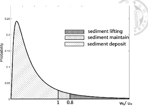
Wu (2015) used the Rouse number 𝑍𝑅 to classify the sediment states (sediment deposit 𝑍𝑅 > 2.5 ; sediment suspend 𝑍𝑅 < 2 ; sediment maintain in the water column 2.5 < 𝑍𝑅 < 2 ). We regard 𝑍𝑅 = 2.5 as the threshold of sediment suspension, where 𝑍𝑅 = 𝑤𝑠⁄(𝜅𝑢∗); 𝑤𝑠 = settling velocity; 𝑢∗ = bed shear velocity; 𝜅 = von Kármán constant
(2.8)
where 𝑑∗ = (∆𝑔/𝜈2)1/3𝑑 = dimensionless diameter of particles; ∆= (𝜌𝑠− 𝜌)/𝜌 ; 𝜌𝑠 = density of particles; 𝜌 = density of fluid; 𝑔 =gravitational acceleration; 𝜈 = kinematic viscosity of fluid; and 𝑑 = diameter of particles. Wu (2015) let 𝜃1 and 𝜃0.8 denote substituting 𝜔𝑠⁄(𝑢∗)=1 and 𝜔𝑠⁄(𝑢∗)=0.8 into equation(2.8) respectively since von Kármán constant κ=0.4.
2 3
* 2 3
* *
( 25 1.2 5) ( s / )
d
w u d
0.8
1.5625*
1
Increasing Probability
In the Gambler’s ruin model, the sediment lifting probability is regarded as the increasing probability. Lifting probability can be represented by the first-order Taylor series expansion according to Wu and Lin (2002). Therefore Wu (2015) presented that the increasing probability (𝑝) can be estimated by the dimensionless shear stress based on equation(2.9).
(2.9)
Decreasing Probability
Wu (2015) applied the definition of depositing events that a sediment particle will deposit when 𝜔𝑠⁄(𝑢∗) > 1 to estimate the decreasing probability. Probability of the depositing event can be equal to P(𝜃 < 𝜃1) , and decreasing probability can be represented as 𝑞 = 1 − P(𝜃 > 𝜃1)
(2.10)
Maintaining Probability
We can easily obtain the formula of maintaining probability (𝑟), as 𝑝 + 𝑞 + 𝑟 = 1 in the Gambler’s ruin problem. Figure 3.1 shows the illustration of different state probability.
(2.11)
2ln 0.0687 /
ln(0.0687 / ) 2
0.5 0.5 1 exp
ln(0.0687 / )) 0.724
L L L
C C
p C
2ln 0.044 /
ln(0.044 / ) 2
0.5 0.5 1 exp
ln(0.044 / ) 0.724
L L L
C C
q C
2
2
ln(0.0687 / ) 2 ln(0.0687 / )
0.5 1 exp
ln(0.0687 / ) 0.724
ln 0.044 /
ln(0.044 / ) 2
0.5 1 exp
ln(0.044 / ) 0.724
L L
L
L L L
C C
r C
C C C
Figure 3.1 Probabilities of different states in gambler ruin model
3.1.3 Characteristics of Flow Field
Before estimating the probability of sediment movement, we first need to obtain the dimensionless shear stress. (𝜃 = 𝑢∗2⁄∆𝑔𝑑, where 𝑢∗=shear velocity; d =diameter of particle). The dimensionless shear stress is a parameter expressing the characteristic of flow field and sediment particle geometric features. Moreover there are several methods to estimate the shear velocity of flow filed. Wu (2015) applied the energy gradient method in the modified Gambler’s ruin model for steady and uniform open channel flow, ( 𝑢∗ = √𝑔𝑅𝑆 ; 𝑅= hydraulic radius; and 𝑆= friction slope). Wu (2015) estimated the bed friction slope by curve fitting; furthermore assumed the discharge of a rating curve can be evaluated by multiplying the depth-average velocity and the cross section area (i.e.,Q = A ∗ 𝑢̅̅̅ where A= cross section area; 𝑢𝑑 ̅̅̅= depth-average velocity). 𝑑 Moreover, he simplified the flow field by the logarithmic velocity profile. As such, the depth-average velocity can be evaluated by integrating the velocity profile
(2.12)
(2.13)
where 𝑢̅̅̅(z)= temporal mean velocity at height z above the bed level; ℎ= water depth; 𝑑 𝑧0=zero-velocity level (𝑧0 = 𝑘𝑠⁄30); 𝑘𝑠= equivalent roughness height of Nikuradse is assumed equal to 2𝑑 in Wu and Chou (2003).
3.1.4 Quantification of Sediment Concentration
After estimating the probability of the Gambler’s ruin model, we also need to quantify sediment concentrations in the water column. It is critical that the number of sediment particles for different state i in the water column above per unit bed area can be calculated by multiplying the mean concentration and water depth. Wu (2015) assumed the sediment concentration following the Rouse profile, and used the logarithmic profile assumption for the flow velocity. Researchers usually use the solid volume per unit fluid volume (𝑚3⁄𝑚3) or the solid mass per unit fluid volume (𝑘𝑔 𝑚⁄ 3) to express sediment concentration. The concentration is expressed as a function of height 𝑧 by the Rouse profile.
(2.14)
where 𝑐𝑎= reference concentration; 𝑎= reference height (𝑎 = 2.75𝑑), which is bed load thickness in Cheng and Chiew (1999).
The depth-integrated suspended load transport (𝑞𝑠,𝑝) can be obtained by integrating the product of flow velocity 𝑢̅̅̅(𝑧) and suspended concentration 𝑐(𝑧) from 𝑎 to ℎ as 𝑑 following
* 0
1ln( ) ut z u z
0 0
* 0
ln( ) ( )
h h t z z d
u z
u z dz z dz
u h h
*( ) *
ws
u a
h z a
c c z h z
(2.15)
Wu (2015) defined the mean volumetric concentration as the following
(2.16)
where 𝑐𝑚𝑒𝑎𝑛= mean concentration ( 𝑘𝑔 𝑚⁄ 3); 𝑞𝑠,𝑝= suspended sediment particle discharge per unit width (𝑘𝑔 𝑠 𝑚⁄ ⁄ ); 𝑞𝑓= flow discharge per unit width (𝑐𝑚𝑠 𝑚⁄ ).
Figure 3.2 Log-profile of flow velocity and Rouse profile of concentration
State 𝑖 is regarded as number of particles equals to 𝑖 in the water column, which can be expressed as the number of particles above per unit bed area (1 𝑚⁄ 2) as the following
(2.17)
* *
,
0
( ) ( ) *( ) ln( )
ws
h h u
s p a t a a
u
h z a z
q u z c z dz c dz
z h z z
, /
mean s p f
c q q
, s mean
s p s
c h
N V
where 𝑉𝑠,𝑝= volume of each suspended sediment particle (𝑉𝑠,𝑝 = 𝜋𝑑3⁄6); 𝜌𝑠= density of particles (𝑘𝑔 𝑚⁄ 3).
In the Gambler’s ruin model, 𝑁𝑠 is defined as the initial state 𝑖 in equation (2.17) by Wu (2015). Moreover, we defined per 1000 particles as one unit since we need to reduce the number of state 𝑖 in order to increase computation efficiency.
3.1.5 Mean Time Spent on Each State
In addition, it is desirable to know the time the concentration will reach a pre-established standard, and the time spent is an important factor of water management.
The gambler’s ruin problems can estimate not only the probability of the gambler reaching a pre-estimate standard but also the mean time spent in each state. If we can exactly define the relationship between the game and the time for each game, we can predict the mean “real time” spent of exceeding events.
Transition probabilities matrix
The transition probability matrix includes probabilities of the transition states. The Gambler’s ruin model is a finite state Markov chain whose states are numbered as T = *1,2,3 … , t+ denotes the set of transient states. Researchers denote the transition probabilities matrix as the following
(2.18)
where 𝐏𝐓 is the transition probabilities matrix. This matrix does not include the state 0 and state 𝑁. For transient state 𝑖 and 𝑗, we denoted 𝑠𝑖,𝑗 as the expected number of time periods that the Markov chain is in state 𝑗, given that it starts in state 𝑖. When 𝑖 = 𝑗 let 𝛿𝑖,𝑗=1, otherwise 𝛿 𝑖,𝑗 is equal to 0. We can express
11 12 1
1 2
t
t t tt
P P P
P P P
PT
(2.19)
and we let 𝐒 denote the matrix of 𝑠𝑖,𝑗 as
(2.20)
We also can express the above equations by using matrix type
(2.21)
Final we can use equation (2.21) to estimate the mean time spent on each state, but the unit of mean time spent is the number of round (one unit of game) in the gambler’s ruin theories. In the engineering application the unit of one simulation time is second or minute, so we need to define the relationship between time and the number of rounds (one unit of game).
3.1.6 The Monte Carlo Simulation of Non-stationary model
The Gambler’s ruin model was developed by deriving an analytical solution in the previous studies. This method would reduce the simulation time. It is hypothesized that probabilities are stationary in each game. The main purpose of this study is building a non-stationary probability model. Analytical solutions are not available under non-stationary probabilities. In this study we applied the Monte Carlo simulation to build a numerical model. Moreover we want to define a relationship between time and the number of rounds of game for defining non-stationary transition probabilities. Later the accuracy of a numerical model will be demonstrated against a stationary case.
Correlation between time and one unit of game
In the Gambler’s ruin theory, the round of games is different from real time. In engineering applications, the real time in the risk analysis needs to be determined.
, , ,
k=1
= t
i j i j ik kj i j ik kj
k
s
P s
P s11 12 1
1 2
t
t t tt
s s s
s s s
S
( )1
T S I P
Before we add the time effect in our model, a relationship to link the round of games and real time needs to be established. It is assumed that the ratio of the number of rounds of games and time is a constant. Such ratio should be influenced by flow condition and sediment characteristics. In this study, this ratio is used to estimate the real time spent, and an appropriate probability can be determined according the time spent.
(2.22)
where the 𝐶𝑡𝑖𝑚𝑒 is the ratio of real time D (day) and the round of a game R(round).
In this study various 𝐶𝑡𝑖𝑚𝑒 values will be tested. Eventually a rule to fit 𝐶𝑡𝑖𝑚𝑒 value is needed in future work. Furthermore, the 𝐶𝑡𝑖𝑚𝑒 value can be determined from experiments with various flow conditions and time scales.
D(day) R(round) Ctime
3.2 Case Study: The Shihmen Reservoir Basin
3.2.1 Property of Research Region
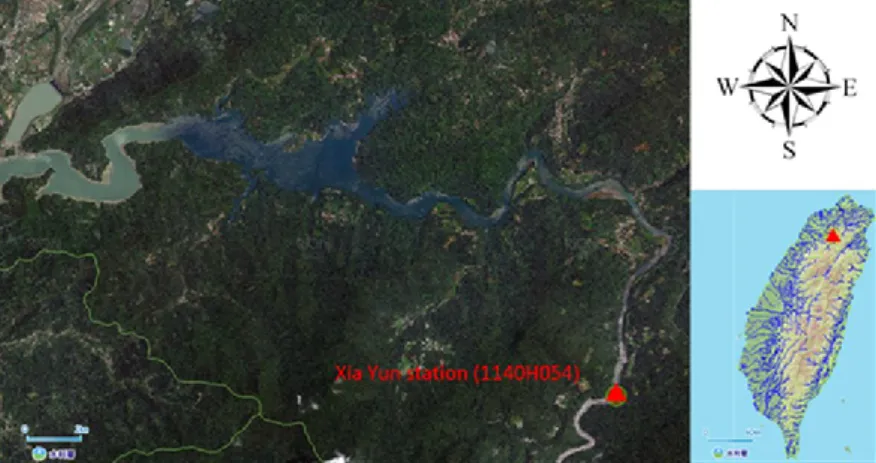
In order to provide a meaningful comparison with the stationary Gambler’s ruin model established by Wu (2015), the Xia Yun hydrologic station (No.1140H054) is selected, for this study. The Xia Yun hydrologic station is located at the upstream side (X:285813, Y:2740336, TWD67) of the Shihmen Reservoir (No.20405) basin as presented in Figure 3.3. The Hydrographic data (i.e. water level, flow discharge, sediment concentration and cross section) in year 2008 were provided by the Northern Region Water Resources Office (NRWRO).
Figure 3.3 Locations of the Xia Yun hydrologic station and Shihmen Reservoir, from Wu (2015)
3.2.2 Data Calibration and Validation
Model calibration needs to be done for our model to determine the friction slope 𝑆.
We use sixty one daily flow discharge data for calibration and validation. We separate those data into two groups. The first group used for calibration has forty one data, and the second group used for validation has twenty data. The result of the friction slope 𝑆 is equal to 0.00135 by using the least squares method. Figure 3.4 shows the results of the flow discharge rating curve in section 3.1.3 by calibration and validation. The R-square
of the flow discharge rating curve verification is 0.9689.
Figure 3.4 Ratting curves of calibration and verification
In our study, the flow field time series data is used to estimate the non-stationary probability. First, we need to demonstrate that the flow field time series data are a non-stationary process. The wavelet spectrum is applied to identify whether the time series data have the properties of the stationary process. A stationary process needs to satisfy a few conditions.
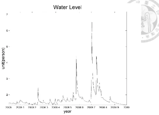
It means that the PDF of time series data is a time independent function. Moreover, the mean and variance are independent of time based on the definition of stationary process. Figure 3.5 shows the water level data of the Xia Yun hydrologic station in 2008.
Figure 3.6 is a wavelet spectrum of water level data. It can be found that period and energy of water level data are changing with respect to time. The mean and variance of the water level with respect to time are not always the same. This result cannot satisfy the definition of a stationary process. In this study, the water level data is demonstrated to be a non-stationary process.
n k m k n m
p(x ,n k,x ,m k) p(x ,n,x ,m)
Figure 3.5 Water level data of Xia Yun hydrologic station in 2008
Figure 3.6 Wavelet spectrum of water level in 2008
3.2.3 Risk Analysis
Wu (2015) applied the maximum standard operating turbidity of water treatment plant (2000NTU) to define the threshold to calculate the risk. Wu (2015) used an empirical formula presented by Hsu et al. (2007) for translation between sediment concentration in the Shihmen Reservoir basin and turbidity as follows
(2.23)
where Q𝑆𝐿,𝑃𝑃𝑀 = sediment concentration [PPM]; Q𝑆𝐿,𝑃𝑃𝑀 = water turbidity. We apply the Gambler’s ruin model to analyze the risk of water turbidity reaching the maximum capacity of water treatment plant (2000NTU). The probability of failure is the probability of event Q𝑚𝑎𝑥 < 𝑄𝑆𝐿,𝑃𝑃𝑀, and thus the risk can be defined as follows
(2.24)
where Q𝑚𝑎𝑥 = maximum sediment capacity of water treatment plant [PPM], and the Q𝑚𝑎𝑥 is equal to 2248 PPM in this study; Q𝑆𝐿,𝑃𝑃𝑀 = estimated sediment concentration [PPM]
3.2.4 Uncertainty Analysis
In the Gambler’s ruin model, the flow field data are an important factor. It is found that using daily water level to calculate the flow field data will incur uncertainty. One of the uncertainties is that using daily mean water level to present the variable flow depth in each day. In this study we consider the uncertainty of variable water level, and we apply the point estimate method (PEM) for the uncertainty analysis. Rosenblueth (1975) presented the two-point method used to calculate the uncertainty of input variable of a deterministic model, and later he improved this method to accommodate asymmetric probability distributions in 1981. The concept of the point estimate (PEM) is using the statistic moments to obtain the representative points of the probability distribution of
,PPM 1.124
SL NTU
Q Q
max ,
( SL PPPM)
Risk P Q Q
each input variable. Equation(2.25) shows the preservation of statistic moments, which is used to obtain the representative points and weight of each representative point.
(2.25)
Based on equation(2.25) we can derive the equations as follow
(2.26)
We used equation (2.26) to obtain the representative points and weight of each point. If we have the statistic moment of input variables, we can estimate the statistic moments of model output by using equation(2.27).
(2.27)
(2.28)
Although the point estimate method (PEM) can quickly calculate the statistic moments of model output, it cannot directly determine the probability distributions of model outputs. In such case, one can be referred to the Monte Carlo method if the probability distribution of model outputs is desirable. The advantage of the point estimate method (PEM) is its computational efficiency.
2 2 2
3 3 3 3
( ) ( )
( ) ( )
+ +
+ X
+ X X
P + P = 1 P x + P x = X
P x X P x X
P x X P x X
2
0.5 1 1 1
1 ( 2)
+
X + X
P
P = 1 P
x X P P
( )n n n
E Y P y P y
2 2
( ) ( ) ( )
Var Y E Y E Y
3.2.5 Results and Discussions
Original Gambler’s Ruin Model
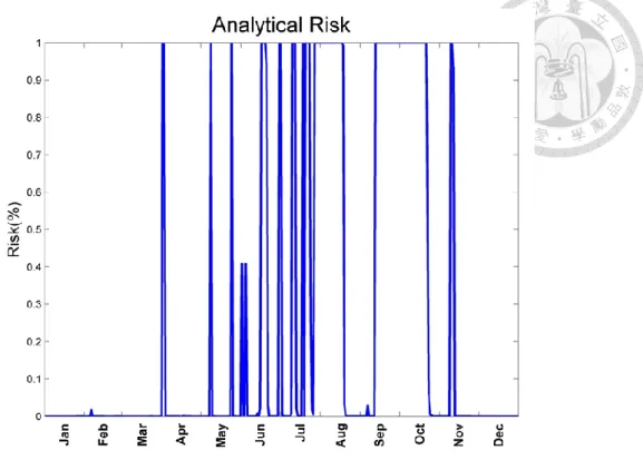
We can calculate the probability of the event that water turbidity exceeding 2248 PPM by using the original Gambler’s ruin model. In the model, only the present flow field and not the change of flow field in the future is considered when quantifying the transition probabilities. Figure 3.7 shows the result of original Gambler’s ruin model.
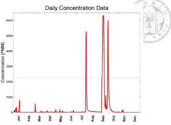
Daily concentration data of the Shihmen Reservoir are compared with the result in Figure 3.8.
Figure 3.7 The risk of water quality exceeding pre-establish standard estimated by original Gambler’s ruin model
Figure 3.8 The sediment concentration data of the Shihmen Reservoir in 2008 The result shows that the water turbidity has high risk in June to October, but original concentration data shows that there are only three water turbidity event higher than 2248 PPM in July to October in the Shihmen Reservoir.
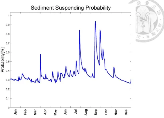
Figure 3.9 Increasing probability in different date
Figure 3.9 shows the sediment lifting probability. It can be observed that before the peak of probability, the probability will decrease very fast. The time scale of extreme flow events in Taiwan is typically not very long so the high lifting probability may not stay for long time. With a stationary transition probability assumption, it is easier that the water turbidity is prone to increase. In this study, it is hoped that the stationary assumption can be relaxed. Then the Gambler’s ruin model is capable of taking to the future flow condition into consideration.
Gambler’s Ruin Model with Non-stationary Probability
The non-stationary Gambler’s ruin model by the Monte Carlo simulation is developed. The proposed analytical solution to the stationary Gambler’s ruin model will be validated. Figure 3.10 shows a stationary simulation by the Monte Carlo simulation, which shows the result is in good agreement with the analytical solution.
Figure 3.10 Risks of original Gambler’s ruin model simulated by the Monte Carlo simulation
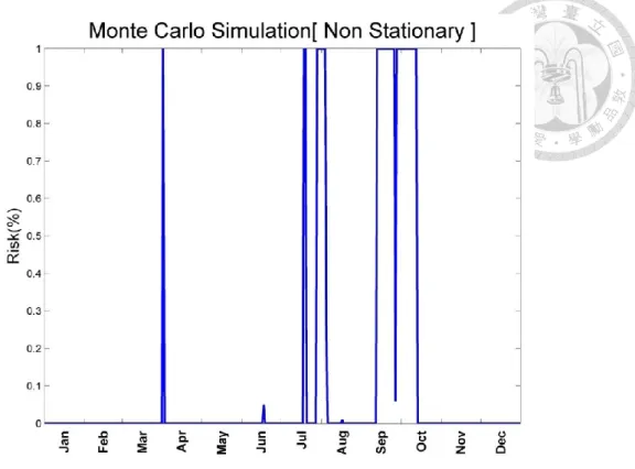
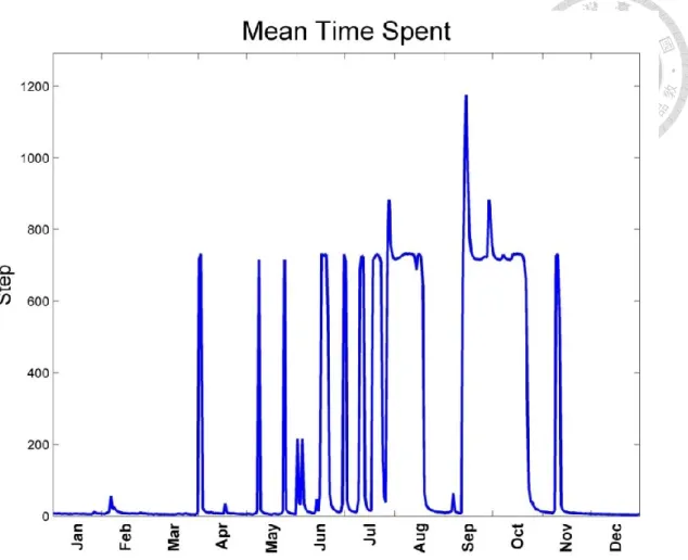
Moreover, we introduce the non-stationary probability model in chapter 3, and the 𝐶𝑡𝑖𝑚𝑒 values are used to consider the transition probability estimated by using future flow condition. Figure 3.12 shows the mean time spent on each state. It can be found that the range of mean time spent is from 200 to 1200 rounds. If the model wants to consider the flow condition within 2-3 days, the ratio needs to be 1⁄500. (round:
200~1200; day:2~3, when 𝐶𝑡𝑖𝑚𝑒~ 1 500⁄ ) Figure 3.11 shows a result of non-stationary probability Gambler’s ruin model with consideration of future flow condition within 2-3 days since range of mean time. The result becomes closer to the real daily concentration data. The non-stationary model needs to have the future flow condition prediction.
Figure 3.11 shows a result when the ratio 𝐶𝑡𝑖𝑚𝑒 is 1 500⁄ .
Figure 3.11 Risks of non-stationary Gambler’s ruin model, which 𝐶𝑡𝑖𝑚𝑒 = 1 500⁄ In this non-stationary probability model we can consider different predicted flow conditions by adjusting 𝐶𝑡𝑖𝑚𝑒 values. However, quantifying the 𝐶𝑡𝑖𝑚𝑒 values as a function of flow and particle conditions is an important task. In this case, the 𝐶𝑡𝑖𝑚𝑒 values are determined according with the mean time spent. The mean time spent shows how many rounds in a simulation, which can offer some information of the ratio 𝐶𝑡𝑖𝑚𝑒. Figure 3.12 shows the mean time spent of the original stationary GR model estimated by the transition probability matrix 𝐏𝐓.
Figure 3.12 The mean time spent of each date
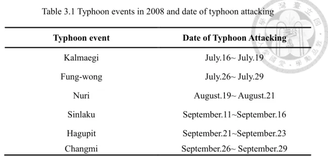
In the non-stationary probability case, 𝐶𝑡𝑖𝑚𝑒 needs to be defined according to the predicted flow condition, which may be simulated by hydraulics channel flood model such as the HEC-RAS. We can observe that the times with high risk are located at July and September, as there are some events of water turbidity reaching the pre-established standard (2248 PPM) in real concentration data. It is found that the date of typhoon striking Taiwan is close to the date of high rick. There are four typhoons attacking Taiwan (refer to Table 3.1). It can be found that the original GR overestimates the risk, since the time scale of typhoon events in year 2008 are not very long. It can be concluded that the GR with non-stationary probabilities is more suitable to estimate the risk of flow turbidity than the original model according to the above results.
Table 3.1 Typhoon events in 2008 and date of typhoon attacking Typhoon event Date of Typhoon Attacking
Kalmaegi July.16~ July.19
Fung-wong July.26~ July.29
Nuri August.19~ August.21
Sinlaku September.11~September.16
Hagupit September.21~September.23
Changmi September.26~ September.29
Result of Rosenblueth Method
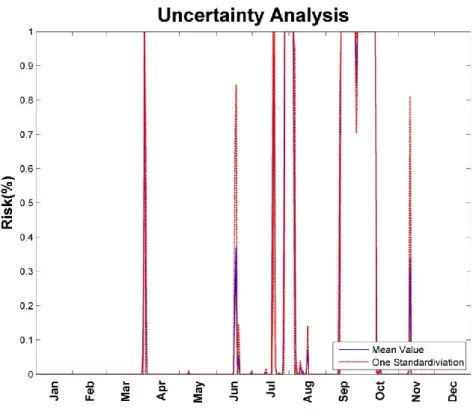
We use hourly data to estimate the uncertainty of the non-stationary model by Rosenblueth point estimate method. We can obtain the mean value and the standard deviation of the output. It can provide information such as what time the flow field is more uncertain. Figure 3.13shows the uncertainty result of non-stationary model. In Figure 3.13 the bold line is the mean value of output and the dash line is one standard deviation of output.
Figure 3.13 Uncertainty result estimated by the Rosenblueth method
The mean value of output is very close to the deterministic result, as the deterministic model uses the mean daily flow data. However, the standard deviations of results are very high, which means the changes of hourly flow data are very huge. We show the error bar result of each four months in the following figures.
Figure 3.14 Uncertainty results from January to March
Figure 3.14 shows the uncertainty results of model from January to March, and the standard deviations are close to zero. The uncertainties of flow field are insignificant from January to March. In Taiwan the rainfall events occur more often in May to November. The change of hourly flow field is dominated by rainfall so the change of flow condition is not obvious from January to March.
Figure 3.15 Uncertainty results from April to June
Figure 3.15 shows the uncertainty results of model from April to June. The standard deviation becomes high in June. The uncertainty of flow increases significantly, which
Figure 3.16 Uncertainty results from July to September
Figure 3.16 shows the uncertainty results of model from July to September. The standard deviation becomes very fluctuating. The uncertainty of daily flow data might be attributed to the frequent typhoons in summer. (Kalmaegi: July.16~ July.19;
Fung-Wong: July.26~ July.29; Sinlaku: September.11~September.16; Jang-Mi:
September.26~ September.29)
Figure 3.17 Uncertainty results from October to December
Figure 3.17 shows the uncertainty results of model from October to December. There are only some incidents close to October, and the uncertainties are negligible in
December. In the uncertainty analysis, it can be found that those high uncertainty events occur in typhoons. In our research we only consider the uncertainty associated with hourly flow change. Therefore, it shows the most uncertainty factor of hourly flow field is typhoon, at the time scale of substantial changes in flow. Tsai et al. (2014) also presented the typhoon event brings significant rainfall, which leads to increased sediment concentrations. It should be recognized that high risk events usually accompanies high uncertainty flow field. Moreover, in this study, the uncertainty of sediment concentrations is assumed to be primarily attributed to the uncertainty of flow.
If there exist more complex flow conditions, many other uncertainty factors can be considered in the uncertainty analysis.
3.3 Summary and Conclusion
The aim of this study is to establish an improved Gambler’s ruin model with non-stationary transition probabilities that can be used to estimate the risk of violating the pre-established turbidity standard. This study also proposed to modify the stationary probability assumption so that the applicability of this model can be expanded. It can be found that original GR will overestimate when the time scale of extreme flow events is not very long. If the temporal change of extreme flow events is not very high, the flow can be viewed as approximately stationary, then averaged stationary transition probabilities can be used. In our case, when extreme flow events in Taiwan are changing dramatically with respect to time, it is more suitable to use non-stationary probabilities in GR. Although the non-stationary GR can more accurately estimate the risk, the ratio 𝐶𝑡𝑖𝑚𝑒 needs to carefully determined for the predicted flow conditions. The ratio 𝐶𝑡𝑖𝑚𝑒 is determined by using mean time spent in this study. It is found that 𝐶𝑡𝑖𝑚𝑒 should be dependent on the characteristic time scale of extreme flow events, which changes from time to time. Therefore, 𝐶𝑡𝑖𝑚𝑒 needs to be linked with the characteristic time scale of extreme flows, which needs to be further investigated.
The result also shows that both the risk and uncertainty are high in summer, and most of which can be attributed to the occurrences of typhoons. In our research, the transition probability can be defined using flow condition and characteristics of sediment particles. It is assumed that the size of particles is uniform in our research.
This study focuses more on the flow conditions, however, the transition probabilities should vary upon many other variables such as rainfall intensity, bed form and erosion effect. It will avoid the risk be dominated by the flow condition. Furthermore, this model can be extended to more complicated flow conditions.
The aim of this study is to establish an improved Gambler’s ruin model with non-stationary transition probabilities that can be used to estimate the risk. In this study, we propose to modify the stationary probability assumption, and extend the applicability of this model. It can be found that original GR will overestimate the risk when the time scale of extreme flow events is not very long. If the change of extreme flow events is not very high, this problem can be resolved by averaging the transition probability. In our case, extreme flow events in Taiwan are changing dramatically so the non-stationary probability GR is more suitable than original GR. Although the non-stationary GR can more accurately estimate the risk, the ratio 𝐶𝑡𝑖𝑚𝑒 needs to be determined and the future flow predictions should be made available. The ratio 𝐶𝑡𝑖𝑚𝑒 is determined by using the mean time spent in this study, but it is found that 𝐶𝑡𝑖𝑚𝑒 is not always a constant due to the time scale of extreme flow events are not always the same. Therefore, 𝐶𝑡𝑖𝑚𝑒 needs to be linked with time scale of extreme flow, and it is a target of our team in the future. It shows the risk and uncertainty both high in summer, and most of those events are caused by the typhoon. In our research the transition probability is define by using flow condition and characteristic of sediment particle, and it is assume that particle is uniform seize in our research. Therefore, the most important role is the flow condition in our model. The definitions of transition probability are not immutable, and it can consider more variable, such as rainfall intensity, bed form and erosion effect. Furthermore, this model can be applied in more complicate flow field.
Part II: Time-Frequency Analysis
Application of Time-Frequency Analysis
Methods to Analyzing Dengue Fever Incidence
in Kaohsiung
Chapter 4 Introduction
4.1 Problem Statement
The dengue fever has become a significant public health burden in the south Taiwan in recent years. Many research of epidemic and public health thought that the high peaks for dengue fever outbreak have a strong connection with hydrology events.
Moreover, both the frequencies of extreme events of dengue fever and hydrology significantly increase due to climate change. The Zika virus (ZIKV) spread by daytime-active Aedes mosquitoes recently impacted Brazil. More and more researchers start to pay attention to the dengue fever disaster in Taiwan. Statistical models to analyze the correlation between dengue fever and some weather factors such as precipitation, temperature and humidity were proposed. Benjamin (2011) used search query surveillance to develop a predict system, and compared three models to predict the number of dengue fever. Chien and Yu (2014) used the Distributed lag nonlinear model (DLNM) to estimate the risk of dengue fever with different weather factors.
Chien and Yu (2014) used the Distributed lag nonlinear model (DLNM), which can consider the delayed effects and non-linear effects, to estimate the risk of dengue fever with different weather factors. Chiu et al. (2014) also calculated the risk of dengue fever by a threshold-based-quantile regression method, which can consider the spatial characteristics of dengue fever. The above studies all used different weather time series data to investigate the correlation with dengue fever, but those weather factors are multiple time scale data. Multiple time scale data are referred to data consisting of different time scales such as daily time scale, weekly time scale and seasonal time scale.
For example, the precipitation time series data consist of different time scale events such as typhoon and East Asian rainy season. Those statistical models cannot
decompose the time series data into different time scale events. Moreover it is suspected that the dengue fever events have some relationships between extreme hydrologic events. In this study, we propose to use the time-frequency analysis to extract extreme events from original data, and discuss the relationships between the dengue fever and different time scaled hydrology events. Finally, we will summarize what hydrologic events play an important role in dengue fever.
4.2 Objectives of Study
This study attempts to obtain the correlation between dengue fever and different time scale hydrologic factors, including precipitation, temperature, humidity and El Niño, by time frequency analysis. We will discuss the comparisons of statistical model and time-frequency analysis. Moreover, there are many novel time frequency analysis methods presented in last decade. In this study, we select three most well-known time frequency analysis methods to analyze, and compare the difference between each time frequency analysis method.
4.3 Overview of thesis
The time frequency analysis is an improvement of the Fourier transform, which overcomes the shortage of the Fourier transform. The time frequency analyses are suitable to apply to non-stationary signals. It is known that most time series data in natural world are non-stationary signals. Some information or trend can be identified by decomposing or expanding the original time series data. First, many different hydrologic factors in this research relevant to the dengue fever are selected.
Simultaneously, we will compare advantages of different transform methods.
(Short-Time Fourier Transform, Wavelet Transform and Hilbert-Huang Transform) At last, we will discuss the spectrum of each factor from different methods. Suggestions
will be made for Center for Disease Control (CDC) from hydrologic perspectives.