Compressive Detection and Localization of Multiple Heterogeneous Events in Sensor Networks
Ruobing Jiang†, Yanmin Zhu†, Hongzi Zhu†, Qian Zhang‡, Jiadi Yu†, Lionel M. Ni‡
†Shanghai Jiao Tong University
‡ Hong Kong University of Science and Technology
†{likeice, yzhu, hongzi, jiadiyu}@sjtu.edu.cn; ‡{qianzh,ni}@cse.ust.hk
Abstract—This paper considers the crucial problem of event detection and localization with sensor networks, which not only needs to detect occurrences but also to determine the locations of detected events and event source signals. It is highly challenging when taking several unique characteristics of real-world events into consideration, such as simultaneous emergence of multiple events, overlapping events, event heterogeneity and stringent requirement on energy efficiency. Most of existing studies either assume the oversimplified binary detection model or need to collect all sensor readings, incurring high transmission overhead.
Inspired by sparse event occurrences within the monitoring area, we propose a compressive sensing based approach called CED, targeting at multiple heterogeneous events that may overlap with each other. With a fully distributed measurement construction process, our approach enables the collection of a sufficient number of measurements for compressive sensing based data recovery. The distinguishing feature of our approach is that it requires no knowledge of, and is adaptive to, the number of occurred events which is changing over time. We have imple- mented the proposed approach on a testbed of 36 TelosB motes.
Testbed experiments and simulation results jointly demonstrate that our approach can achieve high detection rate and localization accuracy while incurring modest transmission overhead.
I. INTRODUCTION
Recent years have witnessed the rapid development of wireless sensor networks, in which each sensor node is able to sense many environmental parameters including temperature, humidity, sound, pressure, etc. Based on the sensor readings, a wide variety of abnormal events can be detected using wireless sensor networks [1]. A lot of real-world event detection applications have been developed, e.g., forest fire alarming [2], border intrusion detection [3], and chemical spill detection [2].
This paper considers the crucial problem of event detection and localization with sensor networks, which not only needs to detect occurrences but also to determine event locations and source signal strengths. When an event occurs, it typically stimulates some kinds of signals that propagate over the space [4] [5]. Sensor nodes close to the event can sense the signal stimulated by the event. By processing the signals received by those sensors, occurrences of the event can be detected. The sink node in the network is responsible for reporting detected events with their locations, and then appropriate measures can be taken in response to the events. Sensor nodes are usually resource constrained, having limited energy and computational power. The performance metrics for event detection in sensor networks include detection rate, localization accuracy and energy efficiency.
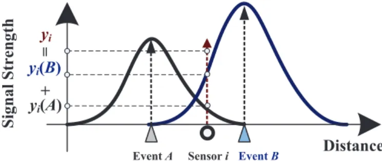
It is highly challenging when taking several unique charac- teristics of real-world events into consideration. First, multiple events may arise at the same time, and even worse, some of the events may have overlapped regions of signal propagation. A sensor located in the overlapped region of two events receives a superimposed signal instead of two separate signals of the two events, as shown in Fig. 1. Second, events are typically heterogenous, differing in the magnitudes of signal strengths caused by the events. It is desirable to determine the nature of each occurred event, e.g., event source signal strength.
Finally, sensor nodes are highly resource constrained and energy efficiency is an important design requirement. This suggests that wireless transmissions should be kept minimal for event detection and localization.
Driven by its importance, there have been a number of research efforts devoted on event detection and localization with sensor networks. A large body of approaches [3] [6]
assume the binary detection model. According to this model, each sensor node has a fixed detection range within which an event can always be detected by the sensor. In the real world, however, such assumption is impractical. With such a simplified model, many sensors may repeatedly report the same event, which adds the difficulty of removing duplicated detections of the same event. On the other hand, it also leads to inaccurate event localization. Several existing studies [7] [8]
[4] have adopted the more realistic model in which an event stimulates a signal whose strength decays over propagation distance. However, they usually require the sink node to collect all signal strengths of the sensors. This incurs high power consumption [9] due to multihop wireless transmissions.
Signal Strength
Distance
Event A Sensor i Event B
yi(A) yi(B) yi
=
+
Figure 1. An example illustrating that a sensor within the overlapped region of two events does not receive two separate signals of events A and B. Instead, it can only read a superimposed signal of the two events.
We have the important observation that event occurrences in a monitoring area are typically sparse in the real world.
Inspired by this observation, we propose a compressive sensing based approach called CED to detection and localization of multiple heterogeneous events. To exploit the sparse nature of events by using compressive sensing, several key issues remain to be solved, including the gap between sparse event occurrences and constrained sensor readings, unknown number of dynamic events, and unfeasibility of single reading serving as a measurement. To address the issues, we first bridge the gap between sparse event occurrences and constrained sensor readings, and then propose a fully distributed measurement construction process enabling the sink to collect a sufficient number of measurements. We also extend the basic CED to reduce the influence of noises. With both testbed experimen- tations and simulations, we demonstrate the efficacy of our proposed approach.
The main technical contributions are summarized as follows.
• We exploit the sparse nature of event occurrences in the real world for detection and localization of multiple heterogenous events which may overlap with each other.
• We propose CED for detection and localization of mul- tiple heterogenous events. It relies only on constrained sensor readings to construct measurements on event occurrences that satisfy the data recovery condition of compressive sensing. The number of occurred events defining the sparsity level of event occurrences, is critical to compressive sensing based estimation, but is dynamic over time and unknown in advance. The distinguishing feature of our approach is that it is distributed and adaptive to the changing number of occurred events.
• We have implemented the proposed approach in a testbed of 36 TelosB motes. Testbed experiments and extensive simulations show that our approach achieves good event detection and localization performance, yet with signifi- cantly reduced transmission overhead.
The rest of the paper is organized as follows. The next section reviews related work. We present the network model and preliminaries in Section III. We explain the basic idea in Section IV, and give the design details in Section V. Section VI reports the implementation and testbed based experiments.
In Section VII, we present simulation results. Section VIII concludes the paper.
II. RELATEDWORK
Event detection under binary detection model. A lot of event detection approaches assume a binary detection model under which an event is considered as detected as long as it occurs within the sensing range of a sensor node. In [6], the binary detection model is adopted and it is assumed that events only occur at some points of interest. In [10], a fault tolerant event detection approach is proposed to increase decision reliability using collaboration between neighboring nodes. In [3], once detecting an event, a sensor node transmits a single pulse instead of a data packet to the sink. The resolution of the event location is limited by the pre-defined size of sectors.
Event detection based on the simplified binary detection model raises the issue of repeated detections and event localization error can be large due to the large detection range.
Event detection under realistic event model. Several existing approaches consider the more practical model for events, in which the signal strength of an event decreases with distance. In [11], an approach is developed for detecting nuclear radiation threat in an open space or a sidewalk in cities. It estimates the location and intensities of threats based on Bayesian algorithms. However, at most one threat is consid- ered. Sheng et al. [7] propose an algorithm for determining the locations of multiple acoustic events. The algorithm requires all sensor readings be collected back to the processing server which then applies maximum likelihood methods to estimate event locations. The main drawbacks of this algorithm include high communication overhead and the requirement on the knowledge of the number of events.
Compressive sensing based event detection. The tech- nique of compressive sensing has been utilized by only sev- eral existing schemes [4] [12] for event detection in sensor networks. However, all of them make direct use of com- pressive sensing. For compressive sensing to be applicable, they assume that the possible locations at which events may occur are known and the number of occurred events is also available. Such assumptions are not realistic in most real-world environments. Furthermore, they also make the impractical assumption that each node is able to monitor every possible location. This essentially means that any event covers the whole monitoring area. This is not true in reality. Therefore, these existing schemes are inapplicable for detection and localization of real-world events that may occur anywhere in the monitoring area, and cover limited region due to quick signal attenuation. More importantly, the number of occurred events is changing over time and unknown in advance. In response to the limitations of the existing schemes, this work proposes a distributed approach based on compressive sensing to address the unsolved challenges.
III. MODEL ANDPRELIMINARIES
A. System Model
We consider a wireless sensor network for detecting and localizing events in a monitoring area, which is composed of a sink node, and a set of connected sensor nodes, denoted by N = {1, 2, · · · , n}. We assume that sensor nodes are uniformly distributed at random in the monitoring area. Sensor nodes are aware of their own locations through embedded Global Positioning System (GPS) receivers or some localiza- tion algorithms [13]. The location of a sensor node i∈ N is denoted by li. The sensor nodes share the same communication range, denoted by r.
Sensor nodes constantly sense the surrounding and record their readings. The sensor network performs event detection and localization periodically. At the beginning of each pe- riod t, all sensors have prepared their readings, y(t) =<
y1(t), y2(t),· · · , yn(t) >. Event detection is performed for
each detection period and the same process is applied for each period. Thus, we omit the period notation t for brevity.
We make the practical assumption that the sensor network is roughly time synchronized. Note that we do not require accurate time synchronization. Many existing algorithms have been developed for practical time synchronization in large- scale sensor networks. For example, FTSP [14] can achieve clock synchronization accuracy as much as 2.24 µs by ex- changing a few bytes among neighbors every 15 minutes.
Since the event detection period is normally tens of seconds to tens of minutes. Thus, FTSP is sufficient for providing the needed time synchronization accuracy.
B. Event Model
Let Ω denote the set of all k events that have occurred in the current detection period, Ω = {ωj}kj=1. Note that k changes over time. As widely used in prior studies such as [7] [8], we model an event ωj as a signal source with source signal strength λj. Events are heterogenous in that the source signal strength is different from event to event. We assume that {λj} are i.i.d. random variables following normal distribution N (µλ, σ2λ). The position of an event ωj is denoted by pj.
The signal strength λj of event ωj attenuates over the distance, as illustrated in Fig. 1. The signal strength at a point that is d(d > 1) away from the signal source is dλα. α is an event-dependent decay factor. When d ≤ 1, the signal strength at the point is λ. To validate the event model, we have performed real experiments on an example event caused by a heater. The experiments shown in Subsection VI-A confirm the applicability of the event model in reality. In our work, we adopt α = 2. However, our design and analysis can be easily extended to other settings of α.
Suppose a sensor node i can sense signals from a subset Ω′ of events in Ω. Its signal reading yi is a superimposed signal strength from events in Ω′
yi= βi
∑
ωj∈Ω′
λj
d2ji, (1)
where djiis the Euclidean distance between sensor node i and event ωj, and βiis the fixed signal gain factor of sensor node i.
Each sensor node i has a signal sensitivity θ below which the sensor cannot detect any signal, i.e., yi = 0 if yi< θ. Based on the sensor sensitivity, an event has a coverage within which a sensor is able to sense the signal from the event.
Definition 1 (Coverage of event). The coverage of an event is defined as the region within which a sensor senses the signal strength from the event that is larger than the sensor’s sensitivity θ.
The monitoring region has an area of ς and is virtually divided into q small grids. The location of an event can be approximated by the centroid of the grid containing the event. Then, we can define a vector to represent the complete information of the events including the number of events, source signal strengths and locations.
Definition 2(Event occurrence vector). The event occurrence vector, denoted by g =< g1, g2,· · · , gq >, represents the occurrences, source signal strengths, and locations of multiple events,
gs=
{ 0, no event in grid s
λj, event ωj ∈ Ω in grid s , 1≤ s ≤ q. (2) Remarks: It is apparent that when there are k events, only k entries of g are nonzero and the rest q− k are zeros.
With Definition 2, we can rewrite (1) as yi = βi
∑q s=1
gs
d2si, (3)
where dsi is the distance between sensor node i and grid s.
Note that the grid size is a design parameter which strikes the tradeoff between event localization accuracy and computation complexity. We will study its impact in Subsection VII-D.
We assume that an event typically lasts for a certain duration before it disappears and the lifetime of an event is larger than the detection period.
C. Basics of Compressive Sensing
We next introduce some basics of compressive sensing [15].
A signal x = [x1, x2,· · · , xn]T ∈ Rn, can be represented on a basis of n× 1 vectors {ψi}ni=1, which are usually orthogonal.
Given an n× n basis matrix Ψ = [ψ1|ψ2| · · · |ψn], x can be represented as the product of Ψ and a coefficient vector d, x = Ψd =
∑N i=1
diψi, in which diis the coefficient for the basis vector ψi. x is said to be k-sparse if the coefficient vector d has no more than k non-zero elements and k≪ n.
Compressive sensing employs a linear measurement process making projections of elements in the k-sparse vector x. Then, x can be recovered based on the projections using algorithms such as the Basis Pursuit algorithm [16].
In the measurement process, a vector z of m measurements ( m < n) are collected, which are inner productions between x and m measurement vectors{ϕi}mi=1,
z = Φx = [ϕT1x, ϕT2x,· · · , ϕTmx]T, (4) where Φ = [ϕ1, ϕ2,· · · , ϕm]T is an m× n measurement matrix. To allow reconstruction of x from the m measure- ments, the m×n matrix Θ = ΦΨ should satisfy the restricted isometry property (RIP) of order 3k [17].
The RIP can be satisfied with high probability either when both conditions C1 and C2 are met, or when both C1 and C3 are met.
• C1: The measurement matrix Φ is a random matrix in which elements ϕi,j are independent and identically distributed (i.i.d.) random variables [17].
• C2: If the measurement matrix does not contain zero values, then the number of measurements should be large enough, i.e., m = O(k log(nk)) [18].
• C3:If the measurement matrix is sparse (i.e., it contains many zero values), the number h of nonzero elements in
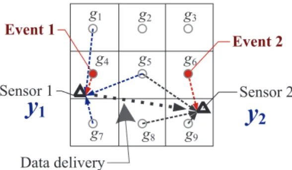
Figure 2. An example for illustrating the basic idea.
each row should be large enough. There is a tradeoff be- tween the number m of measurements and the number h of nonzero elements in each measurement. For example, h = O(log n) suffices if m = O(poly(k, log n)) [19].
IV. BASICIDEA
In this section we explain the basic idea of our compressive sensing based approach. From Definition 2, we can find that to detect and localize the set Ω of k events, it is equivalent to determining the event occurrence vector g. With g, one can obtain the signal strengths λ ={λj}kj=1 of k events and their locations p = {pj}kj=1. Since g is sparse, according to compressive sensing [18], we can fully recover it based on m measurements over g. That is z = Ag, where A is usually an m× q measurement matrix that satisfies condition C1 and C2. In another word, each entry of A should be a nonzero coefficient. Note that m << q, where q =|g|.
Unfortunately, it is difficult to construct measurements of g that satisfy condition C2 using a sensor network, although it is easy to meet condition C1 [5]. This is because there is a clear gap between sparse g and constrained sensor readings. This gap has two implications. First, there is no super node existing in the network, which could project all event occurrences to a single measurement such that each coefficient is nonzero (meeting condition C2). This suggests that we can only seek to constructing measurements meeting condition C3. Second, a single constrained sensor reading is not feasible to serve as a measurement meeting condition C3, because it is only able to provide a superimposed strength from a limited number of events close to it. We call a measurement meeting condition C3 a qualified measurement.
We use the example in Fig. 2 to illustrate this situation.
Suppose Sensor 1 can detect the signal from an event falling in a set of grids, G1 = {1, 4, 5, 7}, and for Sensor 2, G2={5, 6, 8, 9}. We find that the strength reading of Sensor 1 cannot serve as a qualified measurement for g because it is a projection of only g1, g4, g5, and g7.
The basic idea of our approach is to construct m qualified measurements (meeting condition C3),
z =Dg = [DT1g, D2Tg,· · · , DTmg]T, (5) by combining multiple individual sensor readings into each single measurement. To construct a qualified measurement
denoted by zc, 1 ≤ c ≤ m, a set Yc of sensor readings are projected into the measurement.
zc=∑
i∈Yc
yi=∑
i∈Yc
∑
s∈Gi
βigs
d2si = ∑
s∈(∪i∈YcGi) gs ∑
j∈Ns
βj d2sj,
(6) where Gi is the set of grids that can be sensed by sensor i, and Ns is the set of sensors that can sense an event in grid s. Then, there will be|∪
i∈YcGi| nonzero coefficients of g in measurement zc. The coefficient of gs in zc is
D(c, s) = ∑
j∈Ns
βj
d2sj. (7)
For example in Fig. 2, a measurement can be generated by projecting the reading of Sensor 1 and that of Sensor 2. To realize the projection, Sensor 1 transfers its reading to Sensor 2 and Sensor 2 does the projection. Such projection process continues in a distributed fashion. Eventually, a projected value involving a number of sensor readings becomes a qualified measurement and is collected by the sink.
To realize the basic idea described above, we have to address three key issues.
• Unknown number k of events. The number of occurred events as well as the sparsity level of the event occurrence vector is unknown. Without such knowledge, it is difficult to determine the sufficient number of measurements.
Such number of measurements should be adaptive to the changing number of occurred events.
• Quality of measurements. We should determine the sufficient number of sensor readings to be projected in a single measurement which is qualified. Since the sensor network can be in large scale, the measurement constructing process should be executed in a distributed fashion.
• Uncertain coverage of grids. In order to apply com- pressive sensing to estimate g, the measurement matrix D should be known. However, it is uncertain because the coverage of grids are uncertain. The coverage of a grid is defined as the coverage of the event that locates in the grid. Since the event to occur in the grid is unknown, the coverage of the grid is also uncertain.
V. DESIGN OFCED A. Overview
The design of CED is in response to the key issues, realizing the basic idea presented in the previous section. It proceeds in three major stages in each detection period.
(1) In the first stage, to address the key issue of unknown number of events, a specific number of seed nodes are gen- erated. Each seed node initiates a measurement construction process. The generation of the seed nodes is in a distributed fashion and the number of seeds is adaptive to the number of events that have occurred in the monitoring area.
(2) In the second stage, each seed starts a measurement process which leads to a measurement. To address the issue of
ensuring the resulting measurement is qualified, the measure- ment process projects a sufficient number of sensor readings.
Each of the measurement process terminates at the sink which collects the measurement.
(3) In the third stage, after the sink node has collected all the measurements, the sink tries to recover the event occurrence vector g. To address the key issue of uncertain coverage of grids, we propose an iterative algorithm based on the Basis Pursuit algorithm. The algorithm alternates in updating the coverage of each grid by fixing g and estimating g by fixing the coverage of each grid.
B. Generating Seed Nodes
In the first stage, a specific number of seeds should be generated. Each seed node starts the measurement construction process which results in a measurement. The objective of generating the number of seeds is to ensure that a sufficient number m of measurements are eventually collected by the sink, m = O (poly(k, log q)). With CED, the seeds are generated spontaneously and the number of seeds is adaptive to the unknown number k of events that have occurred. The basic idea of the seed generation process is to first generate mp= Θ(k) primary seeds, and then each primary seed selects ms= log q secondary seeds. As a result, the set of all seed nodes includes both the primary seeds and the secondary seeds. It is easy to know the total number m of seed nodes is Θ(k) + Θ(k)× log q = O (poly(k, log q)).
Generating primary seed nodes. At the beginning of each detection period, the primary seeds are spontaneously generated by each node comparing its received signal strength with a threshold, denoted by ρ, which is a design parameter.
If yi> ρ, node i marks itself as a primary seed node.
We next explain the setting of ρ to ensure that Θ(k) primary seeds are generated in the whole network. First, we show that the number of nodes whose signal strength is larger than ρ is normally distributed with parameters that are determined by ρ. Second, we show the determination of ρ by ensuring the probability of generating at least k primary seeds with a customized probability δp, 0.5 < δp< 1.
Theorem 1. The number of primary seeds is a random variable following normal distribution N (f(ρ)k, k(f (ρ)σµλλ)2), f (ρ) = πµρςλn, where ρ is the threshold to generate primary seed nodes.
Proof: Consider an event ω. There is a circular region o(ω) centered at the event, within which the received signal strength is larger than ρ. Assuming the signal gain factors of sensors are 1, the area of o(ω) is πλρω. When k events occur, the total area of the circular regions{oj}kj=1of all the events can be approximated as,
ς(y≥ ρ) = π ρ
∑k j=1
λj. (8)
Because of the uniformly distributed sensor nodes, the expect-
ed number of primary seeds, mp, can be computed as, mp=πn
ρς
∑k j=1
λj. (9)
Because{λj}kj=1are i.i.d. random variables following normal distributionN (µλ, σ2λ), mpis also a random variable follow- ing the normal distribution
N (πnµλ
ρς k, k(πn
ρςσλ)2). (10) Given the normal distribution, we want to make sure that the number of generated primary seeds is larger than k with a high probability which is application specific and can be customized by application developers. Let δpdenote this probability. Then, we can derive the closed form of the desired threshold ρ, as shown by the following theorem.
Theorem 2. Let ρ = nπς ( µλ−√
2σλerf−1(2δp−1)) , 0.5 <
δp< 1, then Pr(mp> k) > δp.
Proof: Denoting the cumulative distribution function (CDF) of a random variable X following normal distribution N (µ, σ2) by FX(x) = Pr(X≤ x), we have FX(x) = 12[1 + erf(√x−µ
2σ2)] and erf(x) = √2π
∫x
0 e−t2dt is the Gauss error function, which is a non-decreasing odd function. Because ρ =nπς (
µλ−√
2σλerf−1(2δp−1))
, we have erf−1(2δp− 1) = µλ−nπρς
√2σλ
, (11)
i.e.,
erf(µλ√−nπρς
2σλ ) = 2δp− 1. (12) Since δp > 0.5, then erf(µλ−
ρς
√ nπ
2σλ ) > 0. Because the error function is nondecreasing and k > 1, we have
erf(
√k(µλ−nπρς)
√2σλ
) > erf(µλ−nπρς
√2σλ
) > 0. (13) As a result, we have
erf(
√k(µλ−nπρς)
√2σλ
) > 2δp− 1. (14) Because
erf(
√k(µλ−nπρς)
√2σλ
) = erf(−k− knπµρςλ
√2knπσρςλ ), (15)
and that the error function is an odd function, we have erf(k− knπµρςλ
√2knπσρςλ ) < 1− 2δp. (16)
As a result, we have
Fmp(k) < 1− δp, (17) which means
Pr(mp≤ k) < 1 − δp. (18)
Path length h = 3 hops
Seed 1 2
y0 y1 y2 Sink
y0+yz=1+y2 Measurement constructing path
0 y0
v =
1 0 y1
v =v +
2 1 y2
v =v +
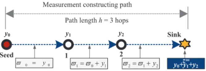
Figure 3. An example for illustrating the measurement construction process which is initiated at the seed node and terminates at the sink.
Thus, we have the conclusion
Pr(mp> k) > δp. (19)
Remarks: The Gauss error function erf(x) defines the CDF of a normally distributed random variable.
Selecting secondary seed nodes.After a sensor marks itself as a primary seed, it tries to recruit a specific number ms of secondary seed nodes from its neighborhood. Each sensor node maintains its neighbors by periodically exchanging heartbeat messages. To recruit ms secondary seed nodes, each primary sensor randomly selects them from its neighbors. Then, it no- tifies the selected nodes by broadcasting a message containing the IDs of the selected secondary seed nodes.
We next show the determination of the important number msof the secondary seeds that a primary seed recruits. Since wireless links in sensor networks are unreliable, measurement processes may fail before they reach the sink node. To account such failures caused by unreliable links, each primary seed node should select a sufficient number of secondary seeds. We assume that the average link reliability of each link is P (after taking into account the maximum number of per-hop retrans- missions). With the number h of hops that a measurement process will travel (to be explained in the next subsection), the success probability of a measurement process is Ph. The objective is to guarantee that the number of successful measurements arriving at the sink per primary seed is larger than log q with a high probability δs which is an application- specific constant. We know that the number of measurements successfully arriving at the sink is a random variable that is binomially distributed with parameter (ms, Ph). Then, by solving the following equation, we can derive ms.
P r(ms> log q) > δs (20) C. Constructing Measurements
In the second stage, qualified measurements are constructed and collected at the sink. To construct a measurement, the measurement process determines a measurement constructing path along which the sensor readings on the path are projected into the measurement. To ensure the resulting measurement is qualified, the number h of hops of the path should be sufficiently large.
Projecting sensor readings. Suppose the measurement constructing path is already determined. Each node along
the path produces an intermediate measurement by projecting all sensor readings of the nodes proceeding itself along the path and its own reading. Then, the eventual measurement is simply the linear projection of all sensor readings. Consider the example shown in Fig. 3. The measurement is initiated at the seed node and the measurement constructing path is (Seed→ 1 → 2 → Sink). The seed node produces the first intermediate measurement ϖ0 = y0. Then, it sends ϖ0
to Sensor 1 which then produces the second intermediate measurement ϖ1 by projecting its reading into ϖ0, i.e., ϖ1= ϖ0+y1= y0+y1. This measurement process continues along the path and terminates at the sink. Eventually, the sink node produces the resulting measurement z =∑2
i=0yi. In order to support the recovery of g, each measurement is associated with a metadata which includes node IDs and locations of all the sensor nodes involved in the measurement.
Determining path length h (hops).To ensure a measure- ment is qualified, h should be sufficiently large. We show the determination of h in the following theorem.
Theorem 3. When h = ςγ1qrlog q
√ θ
µλ, the expected number of nonzero coefficients of g in a measurement is γ1log q, meeting condition C2, where γ1 is a constant.
Proof: In order to ensure that O(log q) grids can be sensed in a measurement process, h should be determined which is the expected number of sensor nodes along a mea- surement constructing path. Considering the sensing area ς(h) covered by h nodes along the path, the expected path length can be computed as h×r2. The width of ς(h) is the expected sensing range of a sensor which is determined by the expected source signal strength µλ and can be computed as 2√µλ
θ . Then the expected number of grids that is covered by ς(h) can be computed as 12hr× 2√µλ
θ /ς′, where ς′ = ς/q is the area of a grid. Thus, we have h = O(log q)ς/rq√µλ
θ . Using a constant γ1 to represent O(log q), we have h =ςγ1qrlog q
√ θ µλ. Remarks: From Theorem 3, we can see that h can be locally computed by each sensor node.
Selecting relays.To ensure that a measurement constructing path travels h hops and finally reaches the sink node, each relay along the path should select the next relay. We assume that each node has established the hop distance to the sink node through some existing methods (e.g., [20]). We next explain how a relay node is selected. Consider node i with hop distance ηi is on the measurement constructing path of measurement zc, 1 ≤ c ≤ m. There are two main steps. In the first step, node i determines the hop distance η of the next relay. The determination of η is dependent on ηi and the number h′ of signal readings having been projected into zc.
η∈
{ηi− 1}, if h − h′ = ηi
{a|a ≤ ηi− 1}, if h − h′ < ηi
{a|a ≥ ηi}, if h − h′ > ηi
(21)
In the second step, a node with its hop distance equaling η is selected. Node i broadcasts its intermediate measurement
with the required η. On receiving it, all the nodes whose hop distance is equal to η starts a backoff timer. The backoff time of node j is inversely proportional to the number of intermediate measurements that it has relayed. As a result, the neighbor having relayed the least number of measurements will first reply an ACK to i. On receiving the ACK, i further notifies the completion of relay selection by a broadcast, muting other competing nodes.
D. Estimating Event Occurrence Vector
In the third stage, the sink node detects the occurrences and the locations of the occurred events by estimating the event occurrence vector with all the received measurements.
We first construct the measurement matrix D based on the metadata of the collected measurements. Then, we propose an iterative algorithm to estimate the event occurrence vector with z andD. Finally, the information about the occurred events is extracted from the estimated event occurrence vector.
Constructing D0. Since the measurement matrixD in (7) is necessary to estimating g but it is unknown, we construct the initial measurement matrixD0by estimating the expected coverage of grids. Suppose the set of sensor nodes involved in measurement zcis Yc, in which a subset Nsof nodes are in the coverage of grid s. Then, we have D0(c, s) =∑
i∈Ns
βi d2si. To compute it, we first determine the subset Nsby initializing the signal strength in grid s as the expected source signal strength µλ. Then, d2si(i ∈ Ns) can be computed using the location information in the metadata.
Designing iterative algorithm. The iterative algorithm alternates in two main steps: updating the measurement matrix D by fixing g and estimating g by fixing D.
Estimating g with D. With a given D, g can be recovered with the Basis Pursuit algorithm [16] by solving,
ˆ
g = arg min
g′ ∥g′∥1, s.t. z =Dg′. (22) UpdatingD with g. Given g computed in the previous step, the signal strength for each grid is updated. Then, the coverage of each grid can be adjusted. Next, D is updated.
The algorithm terminates until the difference between the new computed D and the previous one is smaller than a tiny positive value which is application specific. The pseudo codes of the algorithm are in Algorithm 1.
Detecting and locating events based on g. We finally determine the number k of the occurred events, their locations p ={pj}kj=1, and source signal strengths λ ={λj}kj=1. k is the number of nonzero entries in g. Then, the nonzero entries in g are assigned to λ, and the centroids of the corresponding grids with detected events are assigned to p.
E. Dealing with Noisy Signals
In reality, received signals of sensor nodes usually con- tain noises. Two factors account for such noises, including environmental turbulence and cheap hardware of a low cost sensor. Without considering such noises in sensor readings, our proposed algorithm may suffer degraded performance of event detection and localization.
Algorithm 1: Iterative Estimation Algorithm Input :
z: measurement vector
D0: initialized measurement matrix q: the dimension of the sparse vector g
M : the maximum number of iterations customized by users Output :
ˆ
g : the estimated sparse event occurrence vector 1: D ← D0, ˆg← ⃗0;
2: foriter=1, iter< M do
3: ˆg← find a solution using Basis Pursuit algorithm given D, z, and q;
4: UpdateD′ with ˆg;
5: if∥D′− D∥2is very small then 6: break;
7: else 8: D ← D′; 9: end if 10: end for 11: return ˆg;
In this subsection, we propose noise-aware CED, which extends the basic CED, to reduce the influence of noises in sensor readings. We first model noises in sensor readings and then revise our iterative estimation algorithm by leveraging the Basis Pursuit Denoising algorithm [16].
Modeling noises.We model a noise as a normally distribut- ed random variable ϵi∼ N (µϵ, σ2ϵ) [16] for node i in its signal reading, yi′= yi+ ϵi. Then, measurements z is now presented as zc′ = zc+∑
i∈Ycϵi= zc+ ε, where Yc is the set of sensor nodes involved in measurement zc. Because |Yc| = h and ϵi∼ N (µϵ, σϵ2), we have ε∼ N (hµϵ, hσϵ2).
Revising iterative estimation algorithm. We revise the iterative estimation algorithm by changing the main step of estimating g with D. The key optimization problem (22) is modified to take the added noises into consideration as follows,
ˆ
g = arg min
g′
γ2∥g′∥1+ 1/2∥z − Dg′∥22, (23) where γ2is an application-specific constant. Then, we employ the Basis Pursuit Denoising algorithm [16] to solve the modi- fied problem, which explicitly allows existence of differences between z andDg.
VI. TESTBEDIMPLEMENTATION ANDEXPERIMENTS
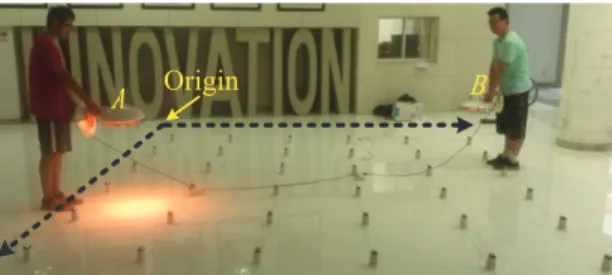
We have implemented our approachCED on a small scale testbed of 36 TelosB motes embedded with a temperature sensor, as shown in Fig. 4. The sink node is connected to a ThinkPad R400 laptop computer. We developed TinyOS based code for sensor nodes, which is responsible for signal sampling, generating seeds, constructing measurements and forwarding intermediate measurements. We also developed Java code at the laptop side to estimate event occurrence vectors, detecting and localizing events. We generated events with electrical heaters as shown in Fig. 5. Two heaters of different rate powers, one is 700 W and the other is 1,000 W.
A. Validation of Signal Attenuation Event Model
We first conduct experiments to validate the signal at- tenuation model for events generated by heaters and derive the attenuation parameter α. In the experiments, a linearly
Origin
Figure 4. The testbed of 36 TelosB motes with two different heater events at A and B.
Figure 5. The linearly-deployed testbed of 20 TelosB motes for validating the signal attenuation event model (the inset shows the heater).
deployed testbed of 20 TelosB motes was used, as shown in Fig. 5. The motes were equally spaced and the separation between two neighboring motes was 20 cm. The heater of 700 W was facing the ground, being elevated 1 meter above the ground. The temperature 1 dm away from the heater is about 60.0°C. The environmental temperature of the day conducting the experiments was about 30.4°C.
Fig.6 plots sensor temperature readings against increasing distance from the heater. The regressed curve of temperature t as a function of distance d is also plotted, t = 30.4 +60d2. We can clear see the regressed curve well sketches the measured readings. This confirms that the signal attenuation event model is valid in reality. In addition, we derive that the attenuation parameter α for heater events is 2.
B. Performance of CED
We next evaluate the performance of CED when there are at most two heterogeneous heater events. The testbed of 36 TelosB motes was deployed over a 5 m×5 m monitoring area.
The separation distance between two neighboring nodes is 8 dm. The origin of the virtual grids is shown in the figure.
Heaters were uniformly placed in the region randomly at random. An event is detected if the estimated location is at most 2 dm away from its real location. We used two settings of virtual grid size: 4 dm and 8 dm. We tested three settings of events: Case 1 (signal event), Case 2 (two separate events), and Case 3 (two overlapping events with average distance of 11 dm). Each data point is averaged over 10 independent experiments with the same configuration.
The detection rate for three cases are reported in Fig 7. We can find that our approach can achieve a detection rate of no lower than 85%. When there is a single event, the detection rate with grid size of 4 dm×4 dm and 8 dm×8 dm are 99% and 93.5%, respectively. The performance of our approach slightly
0 10 20 30 40
30 35 40 45
Distance d (dm) Temperaturet(◦C) Temperature readings
t= 30.4 +60d2
Figure 6. Verifying signal attenua- tion model using a single heat source.
Case 1 Case 2 Case 3
0.6 0.8 1
Three Cases
DetectionRate Grid Size 4 dm × 4 dm
Grid Size 8 dm × 8 dm
Figure 7. Performance results of testbed experiments.
decreases when the grid size is smaller. The main reason is that the number of deployed nodes is limited. As the grid size is smaller, there are more grids, indicating more unknown variables should be estimated.
VII. SIMULATIONS
A. Methodology and Simulation Setup
We conduct extensive simulations to evaluate the basicCED (B-CED) and noise-aware CED (NA-CED) in larger scale settings. They are compared with two existing schemes.
• Complete data collection based scheme (CPLT) [7] : This scheme collects all sensor readings that are beyond sensor sensitivity. After the sink has collected all data readings, it applies the Closest Point Approach (CPA) [7]
to estimate the event occurrence vector. It first identifies all local maxima among all received signals and then selects the closest grid to each local maximum sensor as the location of one occurred event.
• Compressive data collection based scheme (CPRS)[9]:
This scheme uses compressive data collection to recover sensor readings and CPA [7] to detect events. We assume that this scheme knows the priori knowledge about the number k of events (Note it is impractical in reality).
Then, the number of required measurements to recover sensor readings is ϱk log n, where ϱ denotes the average number of sensors within the coverage of an event.
The performance metrics we use for performance evaluation include detection rate, number of false alarms, localization error, source signal strength error, and transmission overhead.
An event is considered as detected if its detected location is within the tolerated location error. Both the localization error and the source signal strength error are calculated as the aver- age difference between the real value and the estimated value for successfully detected events. The transmission overhead counts all transmissions excluding control packets for MAC and routing maintenance.
The default settings of system parameters are as follows.
The number k of events is 10 and they are uniformly dis- tributed at random in the monitoring area. There are 1,000 sensor nodes uniformly distributed in the monitoring area of size 100 m× 100 m. The default size of a virtual grid is 5 m×5 m. The sensor communication range is 10 m. The tolerated location error is 5 m. Both δp and δsare 0.7. γ1 and γ2 are set to 3 and 0.5, respectively. The signal gain factors βi, 1 ≤ i ≤ n are set as 1. The source signal strengths of events follow the normal distribution,N (9, 3). The sensitivity
200 400 600 800 1000 1200 0
0.2 0.4 0.6 0.8 1
Number of Sensor Nodes (n)
DetectionRate
NA-CED B-CED CPLTCPRS
Figure 8. Detection Rate vs. Number of sensor nodes n.
200 400 600 800 1000 1200
0 2 4 6 8 10 12 14
Number of Sensor Nodes (n)
NumberofFalseAlarms
NA-CED B-CED CPLTCPRS
Figure 9. Number of false alarms vs.
Number of sensor nodes n.
200 400 600 800 1000 1200
1.5 2 2.5
Number of Sensor Nodes (n)
LocalizationError
NA-CED B-CED CPLTCPRS
Figure 10. Localization error vs.
Number of sensor nodes n.
200 400 600 800 1000 1200
0 2 4 6 8 10 12
Number of Sensor Nodes (n)
SourceSignalStrengthError
NA-CED B-CED CPLTCPRS
Figure 11. Source strength error vs.
Number of sensor nodes n.
200 400 600 800 1000 1200
102 103 104 105 106
Number of Sensor Nodes (n)
TransmissionOverhead
NA-CED B-CED CPLTCPRS
Figure 12. Transmission overhead vs. Number of sensor nodes n (log scale y-axis).
5 10 15 20
0 0.2 0.4 0.6 0.8 1
Number of Events (k)
DetectionRate
NA-CED B-CED CPLTCPRS
Figure 13. Detection rate vs. Number of events k.
5 10 15 20
0 5 10 15 20
Number of Events (k)
NumberofFalseAlarms
NA-CED B-CED CPLTCPRS
Figure 14. Number of false alarms vs. Number of events k.
2 4 6 8 10 12
0 0.2 0.4 0.6 0.8 1
Side Length of Grid (m)
DetectionRate
NA-CED B-CED CPLTCPRS
Figure 15. Detection rate vs. Grid size.
θ of sensor nodes is set as 0.05. We add Gaussian white noiseN (0, 0.01) to sensor readings. The average transmission success rate of a link is 0.9 and the maximum number of retransmission is 3. Each data point is the average value of 20 independent runs with the same configuration.
B. Impact of Number of Sensor Nodes
We first study the performance of all the schemes as the number of nodes increases from 200 to 1,200. We report the results in Fig. 8 to Fig. 12. We can find that the noise-aware CED consistently achieves the best detection rate, the least false alarms, the lowest transmission overhead, and the modest event localization error and source signal strength error. This confirms that the noise-awareCED successfully leverages the sparsity of event occurrences in the monitoring area.
Compared with the noise-aware CED, the basicCED pro- duces considerably worse detection rate, more false alarms, lower localization error and source signal strength error, and similar transmission overhead. The results demonstrate that the extension for dealing with noises is effective. Signal readings of sensors are associated with noises. Not taking such noises in consideration results in degraded detection rate and increased number of false alarms.
Even granted with the impractical knowledge of number k of occurred events, CPRS still has the worst detection rate, and the highest transmission overhead. It achieves the lowest localization error, and modest number of false alarms and signal strength error because it only detects less than 2 events. It is assumed by CPRS that the sensor readings are sparse but it is usually not true because a single event can cause many nonzero sensor readings. As a result, using a
compressive sensing collection approach fails to accurately recover all sensor readings. This immediately leads to the poor performance of CPRS.
Compared with CPRS, CPLT has a better detection rate, and a lower transmission overhead, but more false alarms, larger localization error and signal strength estimation error.
The main reasons for the poor performance of CPLT are two folds. On the one hand, it is not able to determine the number k of the occurred events. On the other hand, applying the technique of selecting the closest grid to each local maximum sensor as an event suffers low detection accuracy, especially when there are multiple overlapping events.
C. Impact of Number of Events
We next investigate the impact of the number of actually occurred events on the performance of different schemes. In this set of simulations, we vary the number of the occurred events from 2 to 22. We report the results of detection rate and number of false alarms in Fig. 13 and Fig. 14.
We can see that as k increases, both the basic and the noise- aware CED can maintain high detection rate. When k = 22, the detection rates of the basic and the noise-aware CED are 81.1% and 94.3%, respectively. The main reason is that our approach produces a sufficient number of measurements that is adaptive to the number of events. In contrast, CPLT produces decreasing performance of detection rate with increasing k.
This is because more overlapping events result in more local maxima readings that do not respond to true event locations.
As a result, CPLT produces more false alarms as k increases, from 4.1 to 15.4 false alarms.