應用DEMATEL與ANP探討多國藉企業國外直接投資的決定因素：以日本企業投資台灣為例

全文

(1)國立高雄大學經營管理研究所碩士論文. Apply the hybrid of DEMATEL and ANP to explore the determinants of MNEs’ FDI abroad: The case of Japanese enterprises invest in Taiwan 應用 DEMATEL 與 ANP 探討多國藉企業國外直接投資的決定因素：以日本企業投資台灣為例. 研究生：山下大樹撰指導教授：鄭育仁博士. 中華民國一 O 四年一月.

(2) 致謝辭兩年半的時間，總算完成了碩士學位，從一開始的迷迷糊糊到現在寫完這論文，還是覺得不太真實，一路上接受到許許多多的幫助，也有好多好多的感謝，說也說不完。兩年半的時間，總算完成了碩士學位，從一開始的懵懵懂懂到現在寫完這論文，一路過來我受益良多，一路上也受到許多人的幫助，也有說不盡的感謝。最需要感謝的人，就是我的指導教授鄭育仁老師的無私教誨，由於我是日本人留學到台灣念研究所，中文程度在學習研究所課程中算是相當的吃力，但很幸運的是遇見鄭育仁老師，在我不懂或無法消化研究所所學的課程，他總是很有耐心地教導我與指導我的論文，少了老師的幫助，我想或許這篇論文連寫出來的機會都沒有了，有幸能夠在這麼棒的老師指導之下完成碩士學位，真的很榮幸也很感激。此外，特別要感謝各位幫助我完成問卷的日本廠商的人，非常感謝您們撥空時間幫助我完成問卷的填寫，並且提供了許多我在設計問卷時未納入考量的因素並提供寶貴的意見，使我的論文能夠更具備完整性，沒有您們的幫助我的論文也不會順利完成。另外，也相當謝謝兩位口試委員在百忙之中前來我的口試，感謝陳筠昀老師以及林聖蒨老師提供許多讓我的論文能夠更好的建議，使我能夠進一步改善並修正我的論文，在此致上萬分的感謝之意。當然還必須感謝經管所的大家，兩年半的時間如果沒有你們的陪伴，研究所之路絕對不會像我經歷過的那樣精彩，我有困難與疑問之時總是能夠提供許多有用的意見，幫助我度過難關。最後，感謝我的父母親還有各位親朋好友對我的無限支持，家裡總是不干涉我做的任何決定，在我決定來台灣念書時也全力支持我，在我研究所期間遇到學期困難低落時候，總是充滿關心幫助我度過難關，直到至今完成論文。總之，要感謝的人真的太多了，少了你們的幫助，我不可能可以完成這篇論文，真的，非常感謝。山下大樹. i. 2015.1.25.

(3) Apply the hybrid of DEMATEL and ANP to explore the determinants of MNEs’ FDI abroad: The case of Japanese enterprises invest in Taiwan Advisor: Dr. Cheng, Yu-Jen Institute of Business and Management National University of Kaohsiung Student: Taiki Yamashita Institute of Business and Management National University of Kaohsiung. Abstract This study employs a hybrid model that combines decision making trial and evaluation laboratory (DEMATEL) and analytic network process (ANP) to explore the determinants of Japanese MNEs invest in Taiwan. In addition to the four motives (namely Market seeking, Efficiency seeking, Resource seeking, and Strategic-asset seeking) Dunning (1993) classified, this study proposes a new Network seeking motive to catch the Taiwan-Japan historical ties. The determinants of each motive are collected from past literature and opinions of five experts. This study designs a self-structured questionnaire for the pairwise comparison of each determinant in each motive. The respondents are focused on the senior managers of seven Japanese multinational enterprises (MNEs) who are all in charge in foreign direct investment (FDI) affairs in Taiwan. The results show that Efficiency seeking is the most strength-of-influence with other motive. Besides, Network seeking dispatches the strongest influence on the other motives. These results highlight the important roles of Efficiency seeking and Network seeking play in the Japanese MNEs investment in Taiwan. Especially, most Japanese MNEs regard Taiwan as a “step stone”, they will expand to invest in other countries in the future instead of to invest in Taiwan permanently. Keywords: DEMATEL, ANP, Foreign Direct Investment (FDI), Multinational Enterprises (MNEs). ii.

(4) 應用 DEMATEL 與 ANP 探討多國藉企業國外直接投資的決定因素：以日本企業投資台灣為例指導教授：鄭育仁博士國立高雄大學經營管理研究所學生：山下大樹國立高雄大學經營管理研究所. 摘要本文結合決策實驗室分析法(DEMATEL)與網路分析法(ANP)來分析日本多國際企業投資到台灣的決定因素。為深討日本企業投資台灣的投資因素、本文除了引用 Dunning (1993)所分類的尋求市場 (Market seeking)、尋求效率(Efficiency seeking)、尋求資源 (Resource seeking) 與尋求策略性資產(Strategic-asset seeking) 等四個投資動機構面外，還額外增加一個新的尋求網絡 (Network seeking) 構面，用以涵蓋台灣與日本過去特殊的歷史淵源。本文設計了一個自我架構 (self-structured) 的問卷，對每一個投資動機構面中的每一個決定因素進行配對比較 (pairwise comparison)，其訪談對象為七位任職於有直接投資到台灣的日商公司，其總部負責投資台灣業務的資深經理人。研究結果顯示，尋求效率動機與其他動機的交互影響最強，同時，尋求網絡也成為日商投資到台灣最重要的動機影響最大。這些結果突顯出尋求效率與尋求網絡動機扮演日本多國藉企業投資台灣的重要角色。特別是日本多國藉企業將投資台灣視為未來到其他投資國家投資的 “跳板 (step stone) ”，而不是想要永久在台灣投資。. 關鍵字：決策實驗室分析法、網路分析法、國外直接投資、多國藉企業 iii.

(5) Contents Chapter 1 Introduction ..........................................................................................................1 1.1 Research Background ......................................................................................... 1 1.2 Research Motivation and Purpose ..................................................................... 4 1.3 Research Contributions ...................................................................................... 5 1.4 Research Structure ............................................................................................. 6 Chapter 2 Literature Review ........................................................................................ 7 2.1 Entry Mode ......................................................................................................... 7 2.1.1 Exports ............................................................................................................. 8 2.1.2 Contractual Agreements .................................................................................. 8 2.1.3 Joint Ventures (JVs) .......................................................................................... 9 2.1.4 Wholly Owned Subsidiaries ............................................................................. 9 2.2 The Determinants of Foreign Direct Investment ................................................ 9 2.2.1 Market Seeking .............................................................................................. 10 2.2.2 Resource Seeking ........................................................................................... 11 2.2.3 Strategic-asset Seeking .................................................................................. 12 2.2.4 Efficiency Seeking .......................................................................................... 12 2.2.5 Network Seeking ........................................................................................... 13 Chapter 3 Research Methodology ............................................................................. 15 3.1 DEMATEL and ANP Technique .......................................................................... 16 3.1.1 DEMATEL Approach ....................................................................................... 16 3.1.2 ANP Approach ............................................................................................... 16 3.2 Research Procedure .......................................................................................... 17 3.2.1 Set up Research Architecture ........................................................................ 17 3.2.2 Select the Candidate Determinants .............................................................. 17 3.2.3 Create the DEMATEL Questionnaires .............................................................. 19 3.2.4 Create the ANP Questionnaires ..................................................................... 20 iv.

(6) 3.2.5 Date Collection .............................................................................................. 21 3.3 Data Processing Steps ....................................................................................... 22 Chapter 4 Research Results ........................................................................................ 28 4.1 Measuring Relationships among Motives by DEMATEL ................................... 28 4.1.1 Calculate the Direct Relation Average Matrix ............................................... 29 4.1.2 Normalized Direct-relation ............................................................................ 30 4.1.3 Derive the Total Influence Matrix .................................................................. 30 4.1.4 Analysis of DEMATEL ..................................................................................... 31 4.2 Measuring the Priority of Determinants by ANP .............................................. 34 4.2.1. Pairwise Comparison .................................................................................... 34 4.2.2 Super-matrix .................................................................................................. 37 4.2.3 Weights and Ranking of Motives and Determinants ..................................... 38 4.3 Discussion ......................................................................................................... 41 Chapter 5. Conclusion .............................................................................................. 44. Reference ................................................................................................................... 47 Appendix .................................................................................................................... 53. v.

(7) List of Figures Fig. 1.1 Taiwan’s annual GDP and inward FDI amount ................................................ 2 Fig. 2.1 Entry mode MNEs may choose to enter a foreign country ............................. 7 Fig. 4.1 Causal diagram of total relationship ............................................................. 32 Fig. 4.2 Causal diagram of total relationship strategic map ...................................... 33 Fig. 4.3 Taiwan acts as a regional trade hub .............................................................. 42 Fig. 4.4 Flying Geese pattern of economic development in East Asia ....................... 43. List of Tables Table 1.1 Taiwan economic growth rate ..................................................................... 1 Table 1.2 Trends of Taiwan’s Foreign Direct Investment ............................................ 3 Table 1.3 FDI source of Taiwan (2001-2010) by realized FDI ...................................... 5 Table 3.1 Determinants description .......................................................................... 19 Table 3.2 Example of the DEMATEL questionnaire ................................................... 20 Table 3.3 Example of ANP questionnaires ................................................................. 21 Table 3.4 The basic information of the seven Japanese MNEs ................................. 22 Table 3.5 The profile of respondents in the seven Japanese MNEs ............................ 22 Table 4.1 The gives and received influences of each motive ...................................... 32 Table 4.2 The ANP pairwise comparison matrix ( A1 ) ................................................ 35 Table 4.3 The ANP average pairwise comparison matrix ( Aa ) ................................... 36 Table 4.4 The weighted super matrix ( W * ) .............................................................. 37 Table 4.5 The limiting super-matrix ........................................................................... 38 Table 4.6 Weights and ranking .................................................................................. 39 Table 4.7 The price of water and electricity .............................................................. 42. vi.

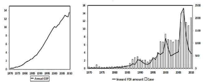
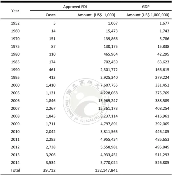
(8) Chapter 1. Introduction. 1.1 Research Background Over the past four decades, Taiwan had experienced one of the world’s highest sustained economic growth (Table 1.1). At the same time, Taiwan’s foreign trade had also grown in a rapid pace. According to Goetz and Hu (1996), economic growth is positively related to capital accumulation. The trend of inward Foreign Direct Investment (FDI) and the gross domestic product (GDP) in Taiwan over 1952-2010 is depicted as Figure 1.1. From Figure 1.1, it can be seen that the amount of inward FDI has a significant influence on economic growth in Taiwan. Thus, inflow FDI is the source of Taiwan’s economic growth. At the period of 1950–2000, the economy of Taiwan had grown at an average rate of 8%. It is a remarkable high growth rate of real per capita GDP. Since then, the economic grow rate declined gradually. In 2007, the approved FDI cases were 2,267 and amount of US$ 15.361 billion, GDP was US$ 408.254 billion (see Table 1.2). Particularly, Taiwan’s inward FDI also reached its peak. After 2007, Taiwan’s inward FDI tends to decline. Table 1.1 Taiwan economic growth rate Year. 1970. 1975. 1980. 1985. 1990. 1995. 2000. 2005. 2010. 2011. 2012. 2013. 2014(f). Rate. 11.51. 6.19. 8.04. 4.81. 5.65. 6.50. 6.42. 5.42. 10.63. 3.80. 2.06. 2.23. 3.43. (f) denotes forecasted data Source: National Statistics, R.O.C. (Taiwan) (http://www.stat.gov.tw/mp, 2015.1.22). 1.

(9) Figure 1.1 Taiwan’s annual GDP and inward FDI amount Source: Statistics on approved overseas Chinese and foreign invest (http://www.moeaic.gov.tw/, 2013.10.13).. Many economists describe the pattern of Taiwan’s economic growth is a “shallow dish economy”, it means Taiwan is an export-oriented country and Taiwan’s economic growth heavily relies on foreign capital accumulation. Therefore, how to attract inward FDI is the major task for the economic agency of Taiwan government. For attracting inward FDI, Taiwan government adopted several investment encouragement incentive strategies such as: tax holidays and tax ceilings in the 1960s, accelerated depreciation in the late 1960s and 1970s, and more-specific depreciation measures and tax credits in the 1980s (Chang and Cheng, 1992). In recent years, Taiwan government promulgated “The Stature for Upgrading Industries” (SUI) on 1991. The main incentive offered by SUI was R&D credit which noted that Taiwan’s corporate income tax has recently been reduced from 25% to 17%. Moreover, The more tax incentives are established on specific areas (e.g., Biotechnology and New Pharmaceutical Industry, Private Participation in Infrastructure Projects, Free Trade Zones, Science Parks, Export Processing Zones, Bonded Factories, and Bonded Warehouses, etc.). SUI had proved its success in bringing about industrial 2.

(10) upgrading and industrial clusters through the provision of tax incentives and the development of industrial zones.. Table 1.2 Trends of Taiwan’s Foreign Direct Investment Year. Approved FDI Cases. GDP. Amount (US$ 1,000). Amount (US$ 1,000,000). 1952. 5. 1,067. 1,677. 1960. 14. 15,473. 1,743. 1970. 151. 139,866. 5,786. 1975. 87. 130,175. 15,838. 1980. 110. 465,964. 42,295. 1985. 174. 702,459. 63,623. 1990. 461. 2,301,772. 166,615. 1995. 413. 2,925,340. 279,224. 2000. 1,410. 7,607,755. 331,452. 2005. 1,131. 4,228,068. 375,769. 2006. 1,846. 13,969,247. 388,589. 2007. 2,267. 15,361,173. 408,254. 2008. 1,845. 8,237,114. 416,961. 2009. 1,711. 4,797,891. 392,065. 2010. 2,042. 3,811,565. 446,105. 2011. 2,283. 4,955,434. 485,653. 2012. 2,738. 5,558,981. 495,845. 2013. 3,206. 4,933,451. 511,293. 2014. 3,534. 5,770,024. 526,805. Total. 39,712. 132,147,841. Source: Statistics on approved overseas Chinese and foreign invest (http://www.moeaic.gov.tw/, 2015.1.22).. On 2010, the newly version of “Statute for Industrial Innovation” (SII) was issued. SII focuses on the interest of creating a fair and competitive tax environment. The areas where tax incentives are offered would need to be revisited. Consequently, under the SII, the only area where tax incentive is still being offered is R&D credit. The main 3.

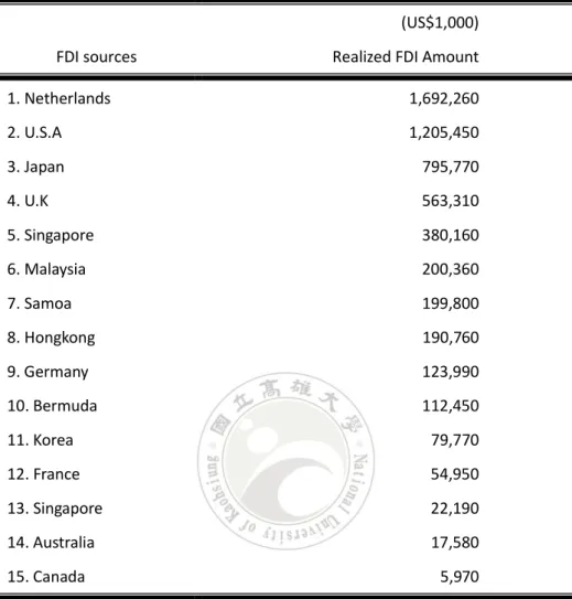
(11) points of the incentive are that the firms may be entitled to a tax credit of up to 15% of the R&D expenditure against its income tax liability. In addition to tax incentives, Taiwan government also established Export Processing Zones, Science Parks, and Free Trade Zones to provide an environment conducive for attracting foreign direct investment and the development of Taiwan’s high-tech industry (Lin et al., 2010).. 1.2 Research Motivation and Purpose However, unilateral policies adopted by host country government can never be a guarantee for successfully attracting inward FDI. The rationale is that MNEs have their own considerations while investing abroad. It is not possible for them to endeavor FDI activities merely according to host country’s incentive measures. After World War II, Taiwan and Japan have close relationship in economic and international trade affairs. This closed relationship is built not only by the geographical proximity between the two countries but also with their historical ties. For the economic development condition, Japan is much advanced than Taiwan. Therefore, Taiwan relies heavily on the investment of Japanese MNEs. From Table 1.3, it can be seen that Japan is ranked third as the source of Taiwan’s realized FDI in the period of 2001-2010. Why should Japanese MNEs still invest in Taiwan while the amount of inward FDI in Taiwan declines? Does Taiwan’s investment environment deteriorate in the eyes of international MNEs? Do Taiwan exist particular attracting factors for raising Japanese enterprises’ willingness to deicide their investment in Taiwan more likely? The above issues are the concerned topics. This study adopts a hybrid of DEMATEL and ANP methodology to explore the. 4.

(12) determinants of Japanese MNEs investing in Taiwan. Table 1.3 FDI source of Taiwan (2001-2010) by realized FDI (US$1,000) FDI sources. Realized FDI Amount. 1. Netherlands. 1,692,260. 2. U.S.A. 1,205,450. 3. Japan. 795,770. 4. U.K. 563,310. 5. Singapore. 380,160. 6. Malaysia. 200,360. 7. Samoa. 199,800. 8. Hongkong. 190,760. 9. Germany. 123,990. 10. Bermuda. 112,450. 11. Korea. 79,770. 12. France. 54,950. 13. Singapore. 22,190. 14. Australia. 17,580. 15. Canada. 5,970. Source: Statistics on approved overseas Chinese and foreign invest (http://www.moeaic.gov.tw/, 2013.10.13).. 1.3 Research Contributions This study explores the critical determinants for Japanese enterprises invest in Taiwan. Research results show that Efficiency seeking locates in the central role with other motives. Network seeking dispatches the strongest influence on the other motives. Strategic-asset seeking receives the strongest influence from the other motives. Only Efficiency seeking motive exists weak inner dependency. Among the overall 16 determinants, the first five determinants for attracting 5.

(13) Japanese MNEs to invest in Taiwan are Step stone, Infrastructure, Geography, History, and Political risk. The most 5 not important determinants are Raw materials, Market size, Population, Market potential, and Cluster. From the above research results, Taiwan economic agency may understand the major consideration of Japanese MNEs while make the decision to invest in Taiwan and therefore proposes suitable attracting measures.. 1.4 Research Structure The remainder of this study is organized as follows: Chapter 2 gives a brief overview of literature related to entry mode and the determinants of FDI and their motives. Chapter 3 introduces the research methodology (DEMATEL and AND) and research procedure. The research results and discussion are shown in chapter 4. Conclusion will be summarized in chapter 5.. 6.

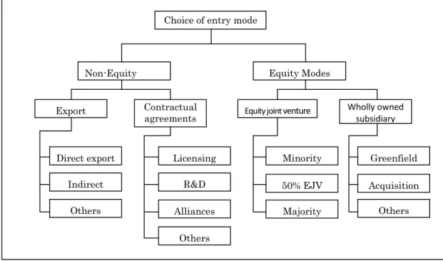
(14) Chapter 2. Literature Review. 2.1 Entry Mode Under the trend of globalization choosing a suitable entry mode is one of the important strategies for MNEs to invest abroad. The decision of how to enter a foreign market can result in a significant impact of MNE’s performance. Pan and Tse (2000) suggested that MNEs can choose a non-equity or equity based mode for entering a foreign country including export, contractual agreements equity joint venture, and wholly-owned subsidiary (depicted as Figure 2.1).. Choice of entry mode. EquityaModes Figure 2.1 Non-Equity Entry mode MNEs may choose to enter foreign country Modes Export. Contractual agreements. Equity joint venture. venture Direct export Indirect export Others. Licensing ngDireexpor R&D t contracts Alliances ng Others. nture. Wholly owned subsidiary subsidiary. Minority. Greenfield. EJV 50% EJV. Acquisition. Majority. Others. EJV. Source: Pan, Y.-G. and D.-K. Tse, 2000, The hierarchical model of market entry modes. Journal of International Business Studies, 31(4), 535-54.. 7.

(15) 2.1.1 Exports Export is used by manufacturing firms to enter a foreign market by shipping the goods and services out of the port of home country. The advantages of export include avoid the costs of establishing a manufacturing operation, enable the firm to some large-scale production, and limit its transport costs (Hill, 2007). 2.1.2 Contractual Agreements Contractual agreements can be classified as licensing/franchising, turnkey projects, contracted R&D, co-marketing (Pan and Tse, 2000). A licensing agreement is an arrangement whereby a licensor grants the intangible property rights to licensees for a specified period, and in return, the licensor receives a royalty fee from the licensees (Hill, 2007). Gillis and Combs (2009) defined that franchising is the franchisee pays royalties to the franchisor, and receive the right to distribute the franchisor’s branded goods or services for a specified period of time in a specific location. For a turnkey project, the contractor agrees to operate all detail of the project for a foreign client, including the training operating personal (Alsakini et al., 2004). The simplest type of contracted R&D is contract research agreements. R&D contracts depend upon the nature of the collaboration, the type of technology, the scope and complexity of the project, and the various aims and objectives of each party. According to Binns and Driscoll (1998), in the R&D agreements, one party will conduct a relatively short-term or simple project in which the experimental protocols and parameters are set by the paying party and the possible outcomes are relatively well-defined. Strategy alliance is based on sharing of vital information, assets, and technology. 8.

(16) between the partners. Although they are often competitors in the product markets, firms frequently form strategic alliances in order to cooperate in some aspects of their business. Actually, this kind of partial cooperation is a common feature among most strategic alliances (Qiu, 2009). 2.1.3 Joint Ventures (JVs) Joint venture is two or more firms collaborate their investment in a new firm, which neither can achieve on its own, for fulfilling a specific objective (Dunning, 1993). Through international joint venture (IJV), MNEs may benefit from the host country’s competitive conditions, culture, language, and political risk (Hill, 2007). Because the equity of joint ventures is shared among partners, the risk of each partner to their share of the investment is limited (Nielsen and Nielsen, 2009). 2.1.4 Wholly Owned Subsidiaries Wholly owned subsidiary entail higher commitment of resources and investments in order to assure full ownership and operational control (Nielsen and Nielsen, 2009). A wholly owned subsidiary is stocked 100 percent of the equity by the MNE. Establishing a wholly subsidiary in foreign market can be done by two ways. They are referred to (1) Greenfield FDI: Invest projects that entail the establishment of new production facilities, such as offices, buildings, plants and factories, as well as the movement of intangible capital (mainly in services). (2) Brownfield FDI: Acquire an established firm in that host country and use that firm to promote its products (Harzing, 2002; World Investment Report, 2006).. 2.2 The Determinants of Foreign Direct Investment What are the determinants for MNEs to invest abroad? Kahouli and Maktouf 9.

(17) (2014) identified the main determinants of FDI in Latin America during the period 1990–2010. They showed that the main determinants positively influence on FDI inflows are trade openness, maintaining low short-term debt levels and presenting a balance of payment deficit, government stability and low expropriation risk. Mukhtar etal. (2014) explored different factors responsible for variation in foreign direct investment to developing countries. They found that openness to the international market, market size, tax rate, exchange rate, infrastructure development, institutions, labor cost, GDP, inflation and political risk are determinants that have significant impact on the flow of FDI towards developing countries or on investor's decision to invest. Dunning (1993) classified MNEs’ FDI motives into four orientations: market seeking, efficiency seeking, resource seeking, and strategic-asset seeking. In addition to surveys the above Dunning motives, this study also discusses a newly classified network seeking. 2.2.1 Market Seeking Large market size is often found in regions with high per capita GDP, implying that more developed areas attract firms with a strong market-seeking orientation. Numerous studies show that FDI flow associates positively with market size and GDP. Kolstad and Wiig (2012) found that host country GDP is significantly associated with Chinese outward FDI. Chinese outward FDI is attracted to countries with large markets. Castro et al. (2013) indicated that the domestic market dimension of Brazil and Mexico is an important factor for attracting FDI. Luo and Tung (2007) concluded that due to their high per capita GDP, most advanced assets are more attracted in more developed regions. Moreover, many research emphasized that market size has a positive and significant effect of outward FDI (Herzer et al., 2008; Chan et al., 2014). 10.

(18) Buckley et al. (2007) studied the relationship between FDI performance and market size, they found that a large market tends to have higher profit opportunities than a small one. Makino et al. (2002) indicated extensively that specify market size is the antecedent that positively impacts FDI location choice. In connection with market size and population, host country’s population and per capita income are found having significant effect on outward FDI (Loungani et al., 2002). 2.2.2 Resource Seeking Resource is defined as physical resource of one kind or human resource. The resource includes most minerals, raw materials (oil, zinc, copper, tin and bauxite.) and agricultural (rubber, tobacco, sugar, bananas, pineapples, palm oil, coffee and tea. Deng (2004) studied investment motivations for Chinese firm to go to overseas. He showed that gaining security over access to raw materials (endowments of natural resources, energy) is often cited as a reason for Chinese firms to invest overseas. Large sources of natural resources are attracted to outward FDI (Kolstad and Wiig, 2012; Ramasamy et al., 2004). Human resource comprises plentiful supplies of cheap and well motivated unskilled or semi-skilled labors. Zhang (2005) investigated the issue by assessing specific assets possessed by Hong Kong and Taiwan investors and China’s location advantages relative to other developing countries. They found that Hong Kong and Taiwan’s direct investment in China was primarily motivated by low labor costs. Bellak et al. (2008) expressed that higher unit labor cost as well as higher total labor cost negatively affect FDI, whereas higher labor productivity impacts positively on FDI. Bartels et al. (2014) examined the characteristics of Location Specific Factors (LSFs) in 11.

(19) Sub-Saharan Africa (SSA). They found that production inputs become the most important factor for FDI followed by political-economic stability. 2.2.3 Strategic-asset Seeking Strategic asset seeking is defined as MNEs aim at acquiring a technological rather than exploiting an existing asset. MNEs pursue strategic operations through the purchase of existing firms and assets for protecting their specific advantages and then to sustain or advance global competitive position. The Strategies asset seeking can be classified as R&D, patent, technology, knowledge, and human resource. Previous study indicated that R&D significant affect MNEs’ outward investment decision. MNEs endeavor in overseas R&D focus on learning from developed countries. Overseas R&D emphasizes its role as knowledge seekers and learners for new and relevant technology (Minin et al., 2012). Human resource of host countries is also a key factor attracting MNEs to undertake R&D activities in host country (Li and Zhong, 2003). 2.2.4 Efficiency Seeking Efficiency seeking is to restructure the existing investments so as to achieve an efficient allocation of international economic activities of the firms. Efficiency seeking MNEs is to take advantage of different factor endowments, large and diversified MNEs producing fairly standardized products and engaging in internationally accepted production. Efficiency seeking can be classified into three elements: host country infrastructure, agglomeration economies, economic of scale. The insufficient development of infrastructure in least developed country raise the operation costs for MNEs while invest in the host countries. Thus, insufficient. 12.

(20) infrastructure has a negative impact on MNEs’ FDI decisions and increasingly arises the costs of attracting investment for host countries (Yamin and Sinkovics, 2009). Thus, the availability of infrastructure in a country definitely can attract inward FDI (Backar et al., 2012; Sun et al., 2010). Combine with specific agglomeration, production costs of MNEs may decline significantly. For host country, specific agglomeration and diverse industry of local division exist positive impact on attracting inward FDI (Chen 2009; Tuan and Linda, 2004). Milner et al. (2006) studied the phenomenon that there exists a large amount of trade between Japan and Mexico for transiting to the U.S. market under NAFTA agreements between Mexico and U.S. They concluded that predominantly production for a non-host country market contains special exporting advantages and facilitates MNEs’ willingness to invest abroad for a third country market. Political risk of host country includes government stability, internal and external conflict, corruption and ethnic tensions, law and order, democratic accountability of government, and quality of bureaucracy are highly significant determinants of outward FDI (Busse and Hefeker, 2006). Kowalewski and Radło (2014) found evidence that foreign direct investment projects undertaken by Polish companies are motivated by the need for efficiency or strategic assets. 2.2.5 Network Seeking In addition to survey the four categories Dunning (1993) had classified, there are still some considerations, e.g., ethnical ties, historical ties, or cultural proximity, which motivate MNEs’ FDI activities. Kubny and Voss (2014) found that the share of local sourcing is similar to other 13.

(21) foreign investors with more extensive forward linkages. Chen et al. (2004) treated local linkages as an investment in local relationships. Chen and Chen (1998) further divided network linkage into internal (intra-firm) and external (inter-firm) linkages. They found that Taiwanese firms are keen on making external linkages, but are indifferent to, or incapable of, making internal linkages through FDI. Taiwanese FDI in the United States is motivated by strategic linkages, but relational linkages facilitate Taiwanese FDI in Southeast Asia and China. Ethnic ties are specific aspects of social networks which are characterized by personal relationship elements such as mother tongue, national origins, ethnic group, and region of birth (Zaheer et al., 2009). Ethnic ties may facilitate FDI location choice, however, ethnic ties do not help to improve firm performance (Jean et al., 2011). Moreover, cultural proximity between host country and MNEs is also an important factor that affects FDI. Pangarkar and Lim (2003) found that cultural proximity has a positive impact on only one performance measure of FDI.. 14.

(22) Chapter 3. Research Methodology. This study focuses on exploring the significant determinants of Japanese MNEs’ FDI abroad in Taiwan. Since the decision making for MNEs to invest abroad concerns several considerations, this study adopts a hybrid multi-criteria based decision-making (MCDM) technique to investigate the major determinants of Japanese MNEs while making their decisions in investing in Taiwan. MCDM is characterized by the ratings of each alternative with respect to evaluate and the weights given to multiple criteria. MCDM is adopted upon knowledge in many fields including mathematics, behavioral decision theory, economics, software engineering, computer technology and information systems, etc. (Koksalan et al., 2011). According to Xiao et al. (2012), classical MCDM methods assume that the ratings of alternatives and the weights of criteria are crisp numbers. The MCDM provides an effective framework for the solution based on the evaluation of multiple conflict criteria. Ou-Yang et al. (2008) declared that a hybrid MCDM model is more suitable in the real world than the previously available methods and helps to measure the mutual importance of each factor. A hybrid MCDM model that combined DEMATEL and ANP can comprehensively solute the dependence and feedback problems, thus can more accurately reflect the real world situations. This study follows the hybrid MCDM model developed by Ou-Yang et al. (2008), which combines the DEMETAL (Decision Making Trial and Evaluation Laboratory) and ANP (Analytic Network Process) methodologies, to evaluate the determinants of Japanese MNEs invest in Taiwan. 15.

(23) 3.1 DEMETAL and ANP Technique 3.1.1 DEMETAL Approach DEMATEL technique was developed by the Science and Human Affairs Program of the Battelle Memorial Institute of Geneva between 1972 and 1976. Fontela and Gabus (1976) proposed that DEMATEL can be used to confirm the relationship between various perspectives and enhance the understanding of the complex issues related to elements concerned. DEMATEL uses matrix calculations to obtain all the direct and indirect causal relationships, as well as the impact strength. However, the DEMATEL technique is not used to confirm the interactions affecting the relationship between the factors. According to Hsu et al. (2013), DEMATEL has been used to research on and to solve a group of complicated and intertwined problems. DEMATEL is particularly popular in Japan, because it is a comprehensive method for building and analyzing a structural model involving causal relationships between complex factors (Wu, 2008). 3.1.2 ANP Approach AHP was proposed by Saaty (1980) as a method for MCDM. According to Alonson and Lamata (2006), AHP is a very popular approach to establish measures in both the physical and social domains that involves qualitative data. The AHP has a special concern with departure from consistency, the measurement of this departure, and with dependence within and between the groups of elements of its structure (Saaty, 2006). However, the AHP does not deal with the interdependences among elements. For dealing with the interdependences among elements, the ANP was proposed as a new MCDM method by Saaty (1996). In the feedback system model of ANP, clusters link one. 16.

(24) by one in turn as a network system (Satty, 2006). This kind of model can capture effectively the complex effects of interplay in human society, especially when risk and uncertainty are involved.. 3.2 Research Procedure This study adopts a hybrid MCDM model combined with DEMATEL and ANP. This method is applied to analyze and form the relationship of cause and effect among evaluation criteria (Ou-Yang et al., 2008). 3.2.1 Set up Research Architecture This study classifies five categories of motives for Japanese enterprises to invest in Taiwan. The first four motives, namely market seeking, efficiency seeking, resource seeking, and strategic-asset seeking, follow from Dunning (1993). The fifth network seeking motive is newly created by this study to catch the Taiwan-Japan historical ties. The determinants in each motive are concluded from past literature survey and interview with five experts who are senior managers of Japanese enterprises work in Taiwan. 3.2.2 Select the Candidate Determinants This study firstly surveys the concerning past literature and select potential candidate determinants. The researcher had an interview with a university professor, Ministry of Economy, Trade and Industry of manager and Japanese MNEs Taiwan branch of manager. After interviewing with experts, the additional potential candidate determinants are collected and rearranged opinions from interview records as: (1) Market size – Although Taiwan’s domestic salary income is about 40% of Japanese origin, it still retains a satisfactory purchasing power; (2) Human resource – Taiwan’s 17.

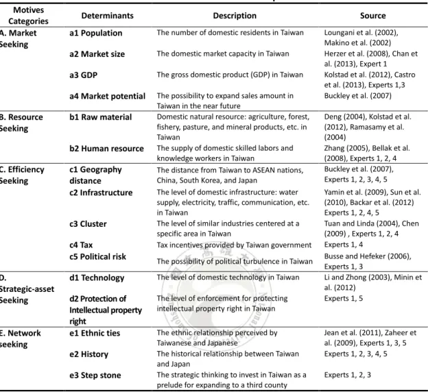
(25) well education system results in part of the skilled labor forces and knowledge workers are globally competitive; (3) A strategic geographical location – Taiwan is located in the middle of Eastern Asia. Average distance from Taiwan to ASEAN countries, Hong Kong, China, Japan, and South Korea is relatively short. It takes about 3 hours to Tokyo or Shanghai, 1 hour to Hong Kong. Taiwan situated as an economic portal to China and to the ASEAN markets; (4) Tax Incentives – Taiwan provides preferential tax incentives and subsidies to MNEs in Taiwan and aims at improving the overall investment environment for recruiting and attracting MNEs; (5) Infrastructure – Infrastructure is able to attract Japanese investment with good physical infrastructure such as water supply, electricity, traffic, communication, etc.; (6) Clustering – Most Japanese MNEs are attracted by Taiwan’s industry clustering, especially, Export Processing Zones and Science Parks Zones becoming important components for attracting Japanese MNEs to invest in Taiwan; (7) Innovation and R&D – Taiwan’s patents per million people ranks first, total patents ranks fourth in the world. Taiwan’s R&D performance can consistently be expected from local research institutes and national universities; and, (8) History – Since Japan had occupied Taiwan for 50 years before World War II, many educated Taiwanese can speak and write Japanese fluently. Japanese MNEs have no difficulty in communication with Taiwanese employees and trading partners. Therefore, Taiwan-Japan historical ties serve as a critical factor for Japanese MNEs’ decision to invest in Taiwan. While collects and rearranges potential candidate determinants from literature survey and export opinions, this study concludes the determinants that are affecting Japanese MNEs to invest in Taiwan and pigeonholes each of those determinants into the five motives categories respectively, showing as Table 3.1. 18.

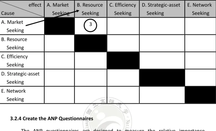
(26) Table 3.1 Determinants description Motives Categories A. Market Seeking. B. Resource Seeking. Determinants a1 Population. The number of domestic residents in Taiwan. a2 Market size. The domestic market capacity in Taiwan. a3 GDP. The gross domestic product (GDP) in Taiwan. a4 Market potential. The possibility to expand sales amount in Taiwan in the near future Domestic natural resource: agriculture, forest, fishery, pasture, and mineral products, etc. in Taiwan The supply of domestic skilled labors and knowledge workers in Taiwan The distance from Taiwan to ASEAN nations, China, South Korea, and Japan The level of domestic infrastructure: water supply, electricity, traffic, communication, etc. in Taiwan The level of similar industries centered at a specific area in Taiwan Tax incentives provided by Taiwan government. b1 Raw material b2 Human resource. C. Efficiency Seeking. c1 Geography distance c2 Infrastructure c3 Cluster c4 Tax c5 Political risk. D. Strategic-asset Seeking. E. Network seeking. Description. The possibility of political turbulence in Taiwan. d1 Technology. The level of domestic technology in Taiwan. d2 Protection of Intellectual property right e1 Ethnic ties. The level of enforcement for protecting intellectual property right in Taiwan. e2 History e3 Step stone. The ethnic relationship perceived by Taiwanese and Japanese The historical relationship between Taiwan and Japan The strategic thinking to invest in Taiwan as a prelude for expanding to a third county. Source Loungani et al. (2002), Makino et al. (2002) Herzer et al. (2008), Chan et al. (2013), Expert 1 Kolstad et al. (2012), Castro et al. (2013), Experts 1,3 Buckley et al. (2007) Deng (2004), Kolstad et al. (2012), Ramasamy et al. (2004) Zhang (2005), Bellak et al. (2008), Experts 1, 2, 4 Buckley et al. (2007), Experts 1, 2, 3, 4, 5 Yamin et al. (2009), Sun et al. (2010), Backar et al. (2012) Experts 1, 2, 4, 5 Tuan and Linda (2004), Chen (2009) , Experts 1, 2, 4 Experts 1, 4 Busse and Hefeker (2006), Experts 1, 3 Li and Zhong (2003), Minin et al. (2012) Experts 1, 5. Jean et al. (2011), Zaheer et al. (2009), Experts 1, 3, 5 Experts 1, 2, 3, 4, 5 Experts 1, 2, 3. 3.2.3 Create the DEMATEL Questionnaires First, this study creates the DEMATEL questionnaire for collecting the cause-effect relationship among the five categories motives while interviewing with selected senior managers of the seven Japanese MNEs. The questionnaires employ a 5-point Likert scale (0 ~ 4) with (0) equaling “No influence”, (1) “Low influence”, (2) “Medium influence”, (3) “High influence”, and (4) “Very high influence”, respectively. The example of the DEMATEL questionnaires and how to fill the comparison of the impact of the five motives categories is shown as Table 3.2. 19.

(27) Table 3.2 Example of the DEMATEL questionnaire ※Please fill out the compared level of the five motives categories in the following table effect A. Market Seeking. Cause A. Market Seeking. B. Resource Seeking. C. Efficiency Seeking. D. Strategic-asset Seeking. E. Network Seeking. 3. B. Resource Seeking C. Efficiency Seeking D. Strategic-asset Seeking E. Network Seeking. 3.2.4 Create the ANP Questionnaires The ANP questionnaires are designed to measure the relative importance between two determinants by pair-wise comparison. After completing DEMATEL questionnaire, interviewee implements ANP questionnaire with the same respondent of the seven Japanese MNEs to collect the relative importance of the dyad determinants while interviewing with selected senior managers of the seven Japanese MNEs. The example of ANP questionnaires is shown as Table 3.3.. 20.

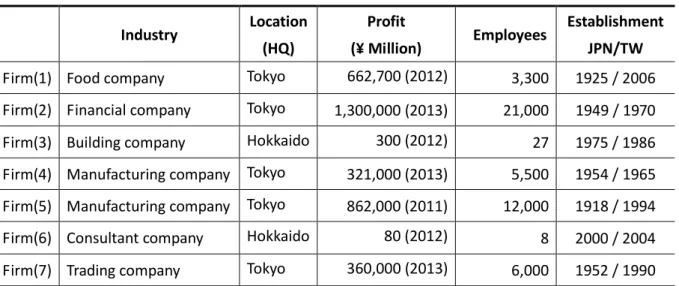
(28) Table 3.3 Example of ANP questionnaire ※Considering the importance of the determinants, fill in 9:1 to 1:9 pairwise comparison. Determinant. i. 9:1. 8:1. 7:1. 6:1. 5:1. 4:1. 3:1. 2:1. 1:1. 1:2. 1:3. Determinant 1:4. 1:5. 1:6. 1:7. 1:8. ✓. a1. a2. ✓. a1. j. 1:9. a3 ……. ✓. a1. b1. (1 = “Equally Important”, 3 = “Moderately Important”, 5 = “Strongly Important”, 7 = “Very Strongly Important”, and. 9 = “Extremely Important”.. 2, 4, 5, and 6 indicated intermediate preferences) 3.2.5 Data Collection This study designs a self-structured questionnaire (see Appendix) for the pairwise comparison of each determinant in each motive. The respondents are focused on the senior managers of seven Japanese MNEs who are all in charge in FDI affairs in Taiwan. The basic information of the seven Japanese MNEs and the profile of every respondent in the seven Japanese MNEs are shown as Table 3.4 and Table 3.5, respectively.. 21.

(29) Table 3.4 The basic information of the seven Japanese MNEs Industry. Location. Profit. (HQ). (¥ Million). Employees. Establishment JPN/TW. Firm(1) Food company. Tokyo. 662,700 (2012). 3,300. 1925 / 2006. Firm(2) Financial company. Tokyo. 1,300,000 (2013). 21,000. 1949 / 1970. Firm(3) Building company. Hokkaido. 300 (2012). 27. 1975 / 1986. Firm(4) Manufacturing company. Tokyo. 321,000 (2013). 5,500. 1954 / 1965. Firm(5) Manufacturing company. Tokyo. 862,000 (2011). 12,000. 1918 / 1994. Firm(6) Consultant company. Hokkaido. 80 (2012). 8. 2000 / 2004. Firm(7) Trading company. Tokyo. 360,000 (2013). 6,000. 1952 / 1990. Table 3.5 The profile of respondents in the Seven Japanese MNEs Industry. Position. Age. Seniority (yrs). Firm(1). Food company. Section Manager. 40 – 50 years. 10 – 20 years. Firm(2). Financial company. Executive Vice President. 50 – 60 years. 20 – 30 years. Firm(3). Building company. President. 30 – 40 years. 10 – 20 years. Firm(4). Manufacturing company. General Affairs H.R.. 40 – 50 years. 20 – 30 years. Firm(5). Manufacturing company. Manager. 40 – 50 years. 20 – 30 years. Firm(6). Consultant company. President. 50 – 60 years. 3 – 10 years. Firm(7). Trading company. Senior Adviser. over 60 years. over 30 years. 3.3 Data Processing Steps The steps of processing the received data summarize as follows: Step 1: Calculate the direct relation matrix All the problematic determinants and strength are extracted for finding the causality. Respondents are asked to make sets of the pairwise comparisons in terms of 22.

(30) influence and direction between determinants. Calculate the direct relation matrix:. d11  d1 j  d1n         D  d i1  d ij  d in            d nj  d nn  d n1 . (1). where d ij indicates the scale of the degree to which the determinant i affects the determinant j . Step 2: Normalizing the direct-relation matrix. On the base of the direct-relation matrix D , the normalized direct-relation matrix X can be obtained through formulas X  SD. (2) 1. S . (3). n. MAX 1 i  n. x j 1. ij. Step 3: Derive the total-relation matrix. Once the normalized direct-relation matrix X is obtained, the total relation matrix T can be acquired by Eq. (4), in which the I is denoted as the identity matrix. Matrix T is the direct/indirect matrix. The ( i, j ) element t ij of matrix T denotes the direct and indirect influence from factor i to factor j .. . . T  lim X  X 2  ...  X k  X I  X  k . 1. (4). Step 4: Calculate the causal diagram. Vector C and vector R, respectively denotes the sum of columns and the sum of. 23.

(31) . rows from total relation matrix T  tij n. Ci   tij i 1 n. R j   tij j 1. n1. ..  j  1,2,..., n. (5). i  1,2,..., n. (6). where ri denotes the row sum of the i th row of matrix T and shows the sum of direct and indirect effects of factor/element i on the other factors/elements. Similarly, c j denotes the column sum of the j th column of matrix T and shows the sum of direct and indirect effects that factor/element j has received from the other factors/criteria. In addition, when i  j (i.e., the sum of the row and column aggregates) (ri  ci ) provides an index of the strength of influences given and received, that is, (ri  ci ) shows the degree of the central role that factor i plays in the problem. If (ri  ci ) is positive, then factor i is affecting other factors, and if (ri  ci ) is negative, then factor i is being influenced (Tamura et al., 2002; Tzeng et. al., 2007). Step 5: Drawing to obtain the inner dependence matrix and impact-relation-map (IRM). In this step, the sum of each column in total relation matrix equals to 1 by the normalization method, and then the inner dependence matrix can be acquired. On the basis of the matrix T , each element ( t ij ) of matrix T provides information about how determinant i affects determinant j . Step 6: Pairwise comparisons matrix In this step, the ANP is used to compare the determinants in whole system to form the supermatrix. According to Satty (1980, 1996), this is done through pairwise comparisons by asking “How much importance/influence does a determinant have 24.

(32) compared to another determinant with respect to our interests or preferences?” In this step, the pairwise comparison matrix is shown as:. 1 a A  aij   21   an1.  .  . Let A  aij. a12  a1n  1  a2 n      an 2  1 . (7). for all i, j  1,2..., n shows a square pairwise comparison matrix, where. a ij gives the relative importance of the determinants i and j . Step 7: Calculate the supermatrix. The general form of the supermatrix can be described as follows: c. 1 e11  e1 m1. e11 e12 1  e1 m1 e21 e22 2  e2 m2. c c W.  c. en1 en 2 2  enmn. W11   W21         Wn1  . . c. 2 e21  e2 n2. c. n en1  enmn. W12. . W1n. W22. . W2 n. . . . Wn 2. . Wnn.              . (8). where Cn denotes the n th motive, emn denotes the m th determinant in the n th motive, and Wij is the principal eigenvector of the influence of the determinants in the j th motive compared to the i th motive. In addition, if the j th motive has no influence on the i th motive, then Wij  0 .. 25.

(33) Step 8: Obtain the weighted supermatrix by multiplying the normalized matrix which is derived according to the DEMATEL technique. According to Ou-Yang et al. (2008), a hybrid method which adopted the DEMATEL technique to solute this problem. First, utilize the IRM to the drive the total influence T.  t11  t1j  t1n       T  ti1  tij  tin       t   t   t   nj nn   n1. n. d i   t ij. (9). j 1. The α-cut total-influence matrix could be normalize and represented as Ts .   t11 t11s  t1sj / d1  t1j / d1  t1n / d1               s Ts   ti1 / d i  tij / d i  tin / d i  =  t i1  t ijs           t  / d  t  / d  t  / d  t s  t s nj 3 nn 3 nj  n1 3  n1.  t1sn     t ins    s   t nn . (10). where t ijs  t ij / d i. . This study adopts the normalized α-cut total-influence matrix Ts and the unweighted supermatrix W . Using Eq. (11) to calculate the weighted supermatrix Ww . Eq. (11) shows these influence level values as the basis of the normalization for determining the weighted supermatrix (Ou-Yang et al., 2008). s t11s  W11 t 21  W12 s s t12  W21 t 22  W22 Ww        t s  W t s  W n1 2n n2  1n.   t ns1  Wij      tijs  Wij  t nis  Win      s   t nn  Wnn . 26. (11).

(34) Step: 9 Limit the weighted supermatrix by raising it to a sufficiently large power k , as Eq. (12) The weighted supermatrix can be raised to limiting power until it has converged and become a long-term stable supermatrix to obtain the global priority vector or called the ANP weighted (Chen et al., 2011).. lim W wk. (12). k . The overall weights are calculated using the above steps to derive a stable limiting supermatrix. Therefore, a model combining the DEMATEL with ANP methods can deal with the problem of interdependence and feedback.. 27.

(35) Chapter 4. Research Results and Discussion. A hybrid MCDM model, which combines DEMATEL and ANP, is proposed to confirm the effect of each motive and determinant presented in this study, and to measure the importance of each determinant related to Japanese MNEs to invest in Taiwan. This chapter presents the results of the analysis of Japanese MNEs investing in Taiwan and the measurement of the relationships among the criteria evaluation. The evaluation modes are based on an interview/questionnaires filled out by senior managers of Japanese MNEs in Japan. 4.1 Measuring Relationships among Motives by DEMATEL DEMATEL questionnaire were asked to specify the relationships between the five motives. The matrix indicates the degree to which the respondent believes motive i affects motive j . For i  j , diagonal elements are set to zero. The researcher collected sample 7 ( H1 ~ H 7 ) to determine how the five motives form a direct relationship matrix.. 28.

(36) 2 2 3 3 3 4 4 4 2 2 2 3 0 0 0 2     0 3 3 3 0 4 4 4 0 3 4 3   4 2 H1  2 3 0 3 3  , H 2  4 4 0 4 4, H 3  4 3 0 3 3 ,       3 2 0 3 4 4 0 4 2 3 0 3 3 4 4 2  4 2 3 2 3 0 4 4 4 4 2 4 4 0 1 3 1 0 1 4 3 3 2 3 3 2 0 0 0 1 2 3 2 3 1  0 2 3 3 0 3 3 3   0   H 4  2 2 0 3 2, H 5  3 3 0 2 2, H 6  3 3 0 3 2 ,       1 2 0 2 2 3 0 2 2 2 0 2 4 1 2 1 2 3 0 2 2 0  2 3 3 0 2 2 2 0  2 4 2 4 0 1 3 2 3   0 H 7  2 3 0 2 3   2 3 0 3 1 2 3 4 3 0 . 4.1.1 Calculate the Direct Relation Average Matrix The procedure is used to calculate the direct relation average matrix, because in order to describe the majority of the MNE's of initial data. Next, the researcher calculated the data from the 7 questionnaire placement in the direct relation matrix to provide on average number of the five motives of matrix. The direct relation average matrix is obtained by averaging the matrices derived from the 7 MNE’s survey data. The average direct matrix is a matrix with zero on the diagonal. For example, matrix D of the first element of the row 1 column 2 is (2 + 3 + 2 + 1 + 1 + 2 + 2) / 7 = 1.857. The average matrix D is shown as. 29.

(37) 0 1.857 3.143 2.571 2.714   2.143 0 2.857 3.183 2.857   D  2.857 3.000 0 2.857 2.714   2.286 2.714 0 2.714 2.714 2.286 2.286 3.000 3.000 0  4.1.2 Normalized Direct-relation According to the previous procedure, it is not practical to know the causal relationship among motives. Thus, this procedure still needs to calculate normalization direct-relationship. The matrix measures according to different scales using a notionally row scale structure is often performed prior to averaging. Normalization may refer to increasingly sophisticated numerical adjustments where by the intention is to bring the entirety of the adjusted values into alignment. Firstly, sum up the values of each row of matrix D . Then, choose the largest value of row sums. Max (10.312, 11.040, 11.429, 10.429, 10.571) = 11.429. By Eqs. (2) and (3), multiplies each value of the matrix D by S . 1 , the 11.429. initial direct influence matrix X can be obtained by normalizing matrix D .. 0 0.162 0.275 0.225 0.238  0.188 0 0.250 0.275 0.250   X  D  S  0.250 0.263 0 0.250 0.238    0.200 0.238 0 0.238  0.238 0.200 0.200 0.263 0.263 0  4.1.3 Derive the Total Influence Matrix After provision of a normalized direct-relation matrix, by Eq. (4), the total influence matrix T is listed as 30.

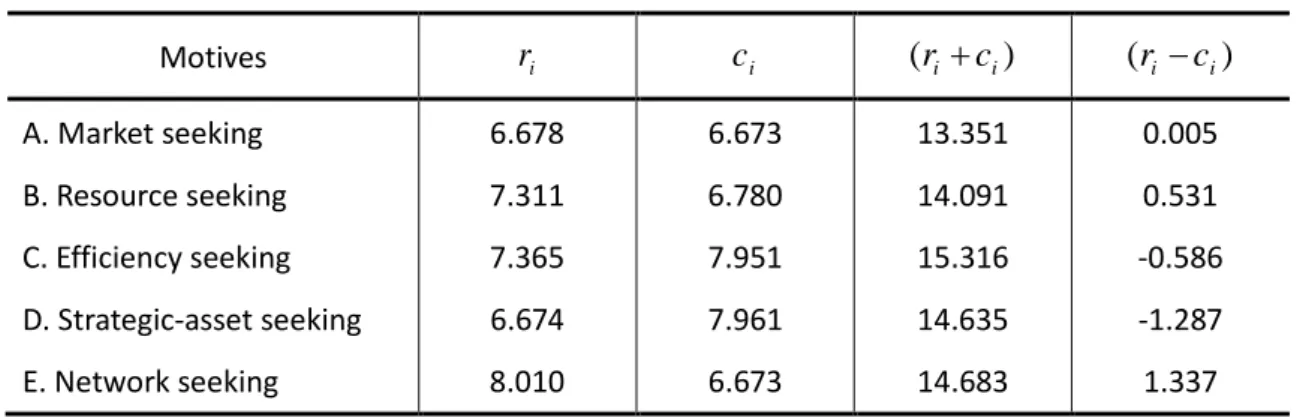
(38) 1.234 1.562 1.489 1.280  1.113 1.385 1.238 1.616 1.687 1.385   T  1.394 1.483 1.460 1.634 1.394    1.297 1.492 1.327 1.279 1.279 1.502  1.528 1.821 1.824 1.335 4.1.4 Analysis of DEMATEL The IRM of the relationships among the motives are shown as Table 4.1, where ri denotes the row sum of the i th row of matrix T and shows the sum of direct and indirect effects of motive i on the other motive. Similarly, c j denotes the column sum of the j th column of matrix T and shows the sum of direct and indirect effects that motive j has received from the other motive. The value of (ri  ci ) indicates the degree of relationship each motive holds along with the other motives. The motive with higher value of (ri  ci ) has stronger relationships with other motives, while the motive with lower value of (ri  ci ) means weaker relationship with other motives. The motives with positive value of (ri  ci ) will influence the other motives greatly, these motives are called dispatchers; however, the motives with negative values of (ri  ci ) are thus greatly influenced by other motives, called receivers. A significantly positive value of (ri  ci ) represents the fact that the motive is known to affect the other motives for more than other motives affecting it. This implies that certain motives should be considered as a priority for maximizing influence (Chen et al., 2011). From matrix T , the gives and received influences of each motive are calculated as Table 4.1.. 31.

(39) Table 4.1 The gives and received influences of each motive. ri. ci. (ri  ci ). (ri  ci ). A. Market seeking. 6.678. 6.673. 13.351. 0.005. B. Resource seeking. 7.311. 6.780. 14.091. 0.531. C. Efficiency seeking. 7.365. 7.951. 15.316. -0.586. D. Strategic-asset seeking. 6.674. 7.961. 14.635. -1.287. E. Network seeking. 8.010. 6.673. 14.683. 1.337. Motives. Observe Table 4.1, it can be seen that the rank of strength-of-influence gives and received (ri  ci ) is motive C (Efficiency seeking: 15.316), E (Network seeking: 14.683), D (Strategic-asset seeking: 14.635), B (Resource seeking: 14.091), A (Market seeking: 13.351); The rank of (ri  ci ) is motive E (Network seeking: 1.337), B (Resource seeking: 0.531), A (Market seeking: 0.005), C (Efficiency seeking: -0.586), D (Strategic-asset seeking: -1.287), respectively. The causal diagram of total relationship is depicted as Fig. 4.1.. 1.5. Network seeking. 1. Market seeking. R-C. 0.5 0. 13. 13.5. Resource seeking 14. 14.5. 15. 15.5. -0.5 -1 -1.5. R+C. Strategic asset seeking. Fig. 4.1 Causal diagram of total relationship. 32. Efficiency seeking.

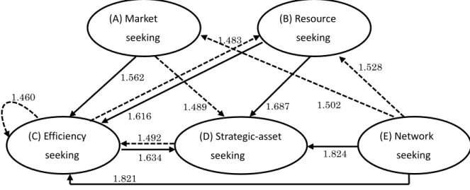
(40) These results reveal that Efficiency seeking, with the highest (r  c) value, has the most relationship with other motives and is located in the central role among motives. Network seeking, with the highest (r  c) value, dispatches the strongest influence on the other motives, is called the “main cause-factor” among the motives; while Strategic-asset seeking, with the lowest (r  c) value, receives the strongest influence from the other motives, is called the “main effect-factor” among the motives. From Table 4.1, it can be used to establish the IRM (also is called causal diagram of total relationship strategic map). Firstly, a threshold is calculated from the elements of matrix T by. t. ij. / 25  1.442 as the screening criteria to eliminate trivial relations. derived from DEMATEL analysis (Liou et al., 2008). In addition, the second quartile (1.394) and third quartile (1.545) are set as separate points to divide weak and strong influence between motives. The strategic map is constructed as Fig. 4.2. The “dotted arrows” denote weak influence between motives, while the “bold solid arrows” represent strong influence. Further observes Fig. 4.2, only Efficiency seeking motive exists weak inner dependency.. (A) Market. (B) Resource. seeking. seeking. 1.483. 1.528. 1.562 1.460 1.616. (C) Efficiency. 1.492. seeking. 1.634. 1.687. 1.489. 1.502. (E) Network. (D) Strategic-asset seeking. 1.824. seeking. seeking. 1.821. Fig. 4.2 Causal diagram of total relationship strategic map (Threshold: 1.442;. Weak. 1.394~ 1.545; Strong 33. 1.545~ 1.824).

(41) 4.2 Measuring the Priority of Determinants by ANP 4.2.1. Pairwise Comparison After applying interview by ANP questionnaire, each determinant is compared pairwisely with respect to its impact on every other determinant. The results are used to create pairwise comparison matrix. A , where. A  a1616  , for all a ij ,. i, j  1,2...,16 represents the relative importance of the determinants i and j .. Since the data collected from every respondent can only fill the upper triangular of a pairwise comparison matrix , ANP assumes that the impact of determinant i affects on determinant. j. is symmetrically reversed of determinant. j. affects on. determinant i . In this sense, the value of each determinant below the diagonal in a pairwise comparison matrix is the reverse value of the symmetric determinant above. / aij . The pairwise comparison matrix of the first respondent the diagonal, i.e., a ji  1 A1 is illustrated as Table 4.2 as an example.. To catch the collective opinion of the seven respondents, the average pairwise comparison matrix of the seven respondents Aa is illustrated as Table 4.3.. 34.

(42) Table 4.2 The ANP pairwise comparison matrix ( A1 ) a1. a2. a3. a4. b1. b2. c1. c2. c3. c4. c5. d1. d2. e1. e2. e3. a1. 1.000. 0.250. 0.333. 0.500. 5.000. 0.500. 0.500. 0.200. 0.167. 0.143. 0.143. 0.125. 0.125. 0.143. 0.143. 0.143. a2. 4.000. 1.000. 0.500. 0.333. 6.000. 0.500. 0.333. 2.000. 0.250. 0.250. 0.143. 0.143. 0.143. 0.250. 0.250. 0.143. a3. 3.000. 2.000. 1.000. 1.000. 7.000. 0.250. 0.333. 0.167. 0.167. 0.143. 0.143. 0.143. 0.143. 0.167. 0.167. 0.143. a4. 2.000. 3.000. 1.000. 1.000. 6.000. 2.000. 2.000. 0.250. 0.250. 0.167. 0.167. 0.167. 0.167. 0.200. 0.200. 0.143. b1. 0.200. 0.167. 0.143. 0.167. 1.000. 0.143. 0.143. 0.143. 0.143. 0.125. 0.125. 0.143. 0.143. 0.143. 0.143. 0.143. b2. 2.000. 2.000. 4.000. 0.500. 7.000. 1.000. 3.000. 0.250. 0.200. 0.167. 0.143. 0.167. 0.143. 0.333. 0.333. 0.333. c1. 2.000. 3.000. 3.000. 0.500. 7.000. 0.333. 1.000. 0.250. 0.250. 0.143. 0.143. 0.143. 0.143. 0.333. 0.333. 0.143. c2. 5.000. 0.500. 6.000. 4.000. 7.000. 4.000. 4.000. 1.000. 0.500. 1.000. 0.200. 0.333. 0.250. 1.000. 2.000. 0.500. c3. 6.000. 4.000. 6.000. 4.000. 7.000. 5.000. 4.000. 2.000. 1.000. 0.333. 0.250. 0.250. 0.250. 0.500. 0.500. 0.250. c4. 7.000. 4.000. 7.000. 6.000. 8.000. 6.000. 7.000. 1.000. 3.000. 1.000. 0.500. 0.500. 0.333. 2.000. 2.000. 1.000. c5. 7.000. 7.000. 7.000. 6.000. 8.000. 7.000. 7.000. 5.000. 4.000. 2.000. 1.000. 3.000. 0.333. 2.000. 2.000. 1.000. d1. 8.000. 7.000. 7.000. 6.000. 7.000. 6.000. 7.000. 3.000. 4.000. 2.000. 0.333. 1.000. 0.500. 2.000. 2.000. 0.500. d2. 8.000. 7.000. 7.000. 6.000. 7.000. 7.000. 7.000. 4.000. 4.000. 3.000. 3.000. 2.000. 1.000. 3.000. 3.000. 3.000. e1. 7.000. 4.000. 6.000. 5.000. 7.000. 3.000. 3.000. 1.000. 2.000. 0.500. 0.500. 0.500. 0.333. 1.000. 1.000. 0.333. e2. 7.000. 4.000. 6.000. 5.000. 7.000. 3.000. 3.000. 0.500. 2.000. 0.500. 0.500. 0.500. 0.333. 1.000. 1.000. 0.333. e3. 7.000. 7.000. 7.000. 7.000. 7.000. 3.000. 7.000. 2.000. 4.000. 1.000. 1.000. 2.000. 0.333. 3.000. 3.000. 1.000. * Note: The Determinants description is given in Table 3.1.. 35.

(43) Table 4.3 The ANP average pairwise comparison matrix ( Aa ) a1. a2. a3. a4. b1. b2. c1. c2. c3. c4. c5. d1. d2. e1. e2. e3. a1. 1.000. 0.763. 0.561. 0.374. 5.917. 0.235. 0.491. 0.279. 0.465. 0.637. 1.155. 0.954. 0.278. 0.126. 0.136. 1.766. a2. 3.250. 1.000. 0.672. 0.252. 5.417. 0.242. 0.325. 0.456. 0.475. 1.088. 0.593. 0.331. 1.154. 0.519. 0.381. 0.942. a3. 2.500. 2.167. 1.000. 0.882. 6.000. 0.964. 0.654. 0.305. 0.597. 0.581. 0.465. 0.445. 0.332. 0.293. 0.332. 1.252. a4. 4.667. 4.833. 2.917. 1.000. 6.500. 2.083. 1.250. 0.482. 2.285. 1.603. 1.139. 2.056. 1.593. 1.428. 1.422. 1.276. b1. 0.461. 0.481. 0.202. 0.165. 1.000. 0.779. 0.451. 0.192. 0.951. 0.137. 0.139. 0.160. 0.150. 0.132. 0.129. 0.285. b2. 5.667. 5.167. 3.875. 0.839. 6.375. 1.000. 2.422. 0.931. 2.252. 0.496. 0.357. 1.056. 0.452. 0.603. 0.607. 1.274. c1. 4.167. 5.500. 3.417. 1.972. 6.250. 1.741. 1.000. 2.208. 2.075. 3.565. 1.914. 2.385. 2.724. 1.660. 1.826. 0.478. c2. 6.667. 6.250. 5.500. 3.667. 6.833. 3.056. 1.271. 1.000. 3.583. 2.889. 3.256. 2.722. 3.750. 1.806. 2.056. 0.549. c3. 4.167. 3.500. 3.167. 2.729. 6.200. 3.229. 2.019. 0.789. 1.000. 0.630. 0.771. 0.653. 1.442. 0.507. 0.658. 0.482. c4. 3.917. 3.542. 3.667. 2.857. 7.500. 3.500. 2.084. 1.049. 3.000. 1.000. 1.972. 1.125. 0.946. 0.750. 0.736. 2.261. c5. 5.194. 3.333. 3.833. 2.708. 7.500. 4.167. 3.519. 1.600. 3.083. 1.354. 1.000. 2.000. 2.389. 0.950. 0.950. 0.922. d1. 4.542. 4.667. 4.667. 2.400. 6.833. 2.556. 2.574. 1.060. 2.167. 1.556. 0.756. 1.000. 1.208. 0.815. 0.913. 0.700. d2. 4.833. 3.367. 4.500. 3.190. 7.167. 4.167. 2.385. 1.477. 2.694. 2.889. 1.076. 1.708. 1.000. 0.796. 0.804. 1.067. e1. 7.833. 3.167. 5.833. 3.028. 7.667. 3.333. 3.354. 2.354. 3.667. 3.750. 1.750. 2.750. 3.889. 1.000. 1.188. 1.243. e2. 7.500. 4.000. 4.833. 3.194. 7.833. 3.167. 3.352. 2.435. 2.333. 4.083. 1.750. 2.417. 3.722. 0.743. 1.000. 1.750. e3. 4.733. 4.375. 3.292. 4.450. 6.333. 3.200. 3.833. 3.667. 3.833. 2.907. 1.917. 2.000. 2.222. 1.063. 1.922. 1.000. * Note: The Determinants description is given in Table 3.1.. 36.

(44) 4.2.2 Supermatrix A supermatrix is a two dimensional matrix that consists of all determinates found in the different motives. The supermatrix represents the influence priority of a determinate at the left of the matrix (row) on a determinate at the top of the matrix (column). First, form an unweighted supermatrix though Eqs. (8)~(10) to obtain the weighted supermatrix Ww (Table 4.4) by multiplying the normalized matrix, which is the weighted supermatrix of the sum of each column given as 1.. Table 4.4 The weighted super matrix ( Ww ) a1. a2. a3. a4. b1. b2. c1. c2. c3. c4. c5. d1. d2. e1. e2. e3. a1. 0.014. 0.016. 0.012. 0.013. 0.063. 0.008. 0.015. 0.015. 0.011. 0.014. 0.072. 0.014. 0.008. 0.009. 0.008. 0.071. a2. 0.031. 0.018. 0.015. 0.008. 0.058. 0.008. 0.007. 0.025. 0.016. 0.048. 0.036. 0.015. 0.047. 0.039. 0.025. 0.059. a3. 0.033. 0.029. 0.019. 0.020. 0.060. 0.011. 0.015. 0.016. 0.021. 0.025. 0.019. 0.021. 0.013. 0.024. 0.023. 0.070. a4. 0.054. 0.080. 0.065. 0.030. 0.061. 0.047. 0.057. 0.026. 0.084. 0.070. 0.068. 0.092. 0.066. 0.038. 0.035. 0.072. b1. 0.002. 0.003. 0.003. 0.005. 0.009. 0.004. 0.006. 0.006. 0.004. 0.005. 0.007. 0.006. 0.005. 0.010. 0.009. 0.020. b2. 0.079. 0.091. 0.088. 0.029. 0.069. 0.031. 0.043. 0.051. 0.083. 0.020. 0.020. 0.044. 0.018. 0.052. 0.048. 0.096. c1. 0.065. 0.117. 0.076. 0.035. 0.067. 0.064. 0.039. 0.115. 0.076. 0.108. 0.122. 0.115. 0.115. 0.146. 0.149. 0.024. c2. 0.084. 0.108. 0.099. 0.091. 0.071. 0.077. 0.052. 0.047. 0.077. 0.085. 0.135. 0.101. 0.139. 0.146. 0.163. 0.040. c3. 0.065. 0.058. 0.050. 0.051. 0.067. 0.077. 0.055. 0.043. 0.031. 0.027. 0.028. 0.029. 0.060. 0.030. 0.041. 0.035. c4. 0.062. 0.045. 0.057. 0.074. 0.071. 0.112. 0.096. 0.058. 0.056. 0.037. 0.041. 0.047. 0.039. 0.065. 0.059. 0.058. c5. 0.071. 0.058. 0.084. 0.086. 0.072. 0.130. 0.110. 0.089. 0.112. 0.060. 0.054. 0.090. 0.095. 0.077. 0.072. 0.045. d1. 0.073. 0.077. 0.073. 0.081. 0.067. 0.089. 0.073. 0.057. 0.062. 0.062. 0.038. 0.041. 0.048. 0.065. 0.062. 0.041. d2. 0.073. 0.063. 0.084. 0.092. 0.071. 0.124. 0.072. 0.080. 0.069. 0.077. 0.059. 0.067. 0.036. 0.068. 0.064. 0.079. e1. 0.109. 0.062. 0.103. 0.109. 0.071. 0.081. 0.094. 0.123. 0.130. 0.108. 0.091. 0.118. 0.130. 0.074. 0.097. 0.093. e2. 0.109. 0.080. 0.099. 0.115. 0.072. 0.075. 0.094. 0.118. 0.081. 0.123. 0.091. 0.110. 0.123. 0.064. 0.069. 0.132. e3. 0.076. 0.092. 0.073. 0.159. 0.052. 0.063. 0.171. 0.131. 0.087. 0.130. 0.118. 0.090. 0.059. 0.093. 0.076. 0.064. * Note: The Determinants description is given in Table 3.1.. 37.

(45) The weighted supermatrix Ww needs to converge and become a long-term stable supermatrix for obtaining the global priority vector. By Eq. (12), the weighted supermatrix Ww is multiplied with itself multiple times to raises to the nth power until the convergence occurs. While the weighted supermatrix is multiplied with itself multiple times, the limiting supermatrix W * is obtained (Table 4.5). The limiting supermatrix is a stable supermatrix reveals the global priority/influentience, .. Table 4.5 The limiting supermatrix ( W * ) a1. a2. a3. a4. b1. b2. c1. c2. c3. c4. c5. d1. d2. e1. e2. e3. a1. 0.043. 0.043. 0.043. 0.043. 0.043. 0.043. 0.043. 0.043. 0.043. 0.043. 0.043. 0.043. 0.043. 0.043. 0.043. 0.043. a2. 0.035. 0.035. 0.035. 0.035. 0.035. 0.035. 0.035. 0.035. 0.035. 0.035. 0.035. 0.035. 0.035. 0.035. 0.035. 0.035. a3. 0.042. 0.042. 0.042. 0.042. 0.042. 0.042. 0.042. 0.042. 0.042. 0.042. 0.042. 0.042. 0.042. 0.042. 0.042. 0.042. a4. 0.055. 0.055. 0.055. 0.055. 0.055. 0.055. 0.055. 0.055. 0.055. 0.055. 0.055. 0.055. 0.055. 0.055. 0.055. 0.055. b1. 0.012. 0.012. 0.012. 0.012. 0.012. 0.012. 0.012. 0.012. 0.012. 0.012. 0.012. 0.012. 0.012. 0.012. 0.012. 0.012. b2. 0.057. 0.057. 0.057. 0.057. 0.057. 0.057. 0.057. 0.057. 0.057. 0.057. 0.057. 0.057. 0.057. 0.057. 0.057. 0.057. c1. 0.089. 0.089. 0.089. 0.089. 0.089. 0.089. 0.089. 0.089. 0.089. 0.089. 0.089. 0.089. 0.089. 0.089. 0.089. 0.089. c2. 0.097. 0.097. 0.097. 0.097. 0.097. 0.097. 0.097. 0.097. 0.097. 0.097. 0.097. 0.097. 0.097. 0.097. 0.097. 0.097. c3. 0.046. 0.046. 0.046. 0.046. 0.046. 0.046. 0.046. 0.046. 0.046. 0.046. 0.046. 0.046. 0.046. 0.046. 0.046. 0.046. c4. 0.066. 0.066. 0.066. 0.066. 0.066. 0.066. 0.066. 0.066. 0.066. 0.066. 0.066. 0.066. 0.066. 0.066. 0.066. 0.066. c5. 0.077. 0.077. 0.077. 0.077. 0.077. 0.077. 0.077. 0.077. 0.077. 0.077. 0.077. 0.077. 0.077. 0.077. 0.077. 0.077. d1. 0.053. 0.053. 0.053. 0.053. 0.053. 0.053. 0.053. 0.053. 0.053. 0.053. 0.053. 0.053. 0.053. 0.053. 0.053. 0.053. d2. 0.074. 0.074. 0.074. 0.074. 0.074. 0.074. 0.074. 0.074. 0.074. 0.074. 0.074. 0.074. 0.074. 0.074. 0.074. 0.074. e1. 0.077. 0.077. 0.077. 0.077. 0.077. 0.077. 0.077. 0.077. 0.077. 0.077. 0.077. 0.077. 0.077. 0.077. 0.077. 0.077. e2. 0.078. 0.078. 0.078. 0.078. 0.078. 0.078. 0.078. 0.078. 0.078. 0.078. 0.078. 0.078. 0.078. 0.078. 0.078. 0.078. e3. 0.101. 0.101. 0.101. 0.101. 0.101. 0.101. 0.101. 0.101. 0.101. 0.101. 0.101. 0.101. 0.101. 0.101. 0.101. 0.101. * Note: The Determinants description is given in Table 3.1.. 4.2.3 Weights and Ranking of Motives and Determinants From the limiting supermatrix, the global weights of motives and local weights of. 38.

(46) determinants are rearranged in Table 4.6. From Table 4.6, it can be seen that Efficiency-seeking (0.374) motive ranks first, Network-seeking (0.256) the second, the third is Market-seeking (0.174), the fourth is Strategic asset seeking (0.126), and Resource seeking (0.069) ranks fifth.. Table 4.6 Weights and ranking Motives. Determinants. Local weight Global weight. A. Market seeking. 0.174 (3) a1 Population. 0.246. 0.0429. 14. a2 Market size. 0.201. 0.0351. 15. a3 GDP. 0.238. 0.0416. 8. a4 Market potential. 0.314. 0.0548. 12. B. Resource seeking. 0.069 (5) b1 Raw material. 0.175. 0.0120. 16. b2 Human resource. 0.825. 0.0568. 9. C. Efficiency seeking. D. Strategic asset seeking. Ranks. 0.374 (1) c1 Geography. 0.237. 0.0885. 3. c2 Infrastructure. 0.258. 0.0967. 2. c3 Cluster. 0.122. 0.0455. 13. c4 Tax. 0.177. 0.0662. 8. c5 Political risk. 0.206. 0.0772. 5. d1 Technology. 0.126 (4) 0.417. 0.0527. 11. 0.583. 0.0736. 7. d2 Protection of intellectual property right E. Network seeking. 0.256 (2) e1 Ethnic ties. 0.301. 0.0771. 6. e2 History. 0.304. 0.0779. 4. e3 Step stone. 0.395. 0.1013. 1. 39.

(47) In addition, Table 4.6 shows that among the overall 16 determinants, Japanese MNEs believe that Step-stone with a weight of 0.101 is the determinant with the first priority. It means, Taiwan plays the role of midway that most Japanese MNEs invest in Taiwan will expand to other countries in the future instead of to invest in Taiwan permanently. Especially, many respondents expressed in the interview that their companies plan to or had already formed joint venture with Taiwanese company to invest in China. Infrastructure (0.097) is followed in the second place. Infrastructure can be ranked in high priority is account for its ability to provide convenient water, electric, traffic, communication, etc. for Japanese MNEs compared to adjacent Asia countries. The third is Geography (0.089). Geographic distance among Taiwan and adjacent Asia countries is much shorter, and can significantly reduce transportation costs of raw materials and final products and the costs of acquiring information from the home country. The fourth determinant is History (0.078). History is an important determinant for Japanese MNEs. Since Japan had ruled Taiwan for fifty years before WWII, many Taiwanese entrepreneurs can speak Japanese fluently, and can also fully understand Japanese culture and lifestyle. Therefore, Japanese MNEs may easily communicate with Taiwanese and perceive their friendship. The fifth determinant is Political risk (0.077). The political situation in Taiwan is relative stable. No hostile political turbulence or terroristic attack happened in Taiwan. Most of the 5 unimportant determinants are concentrated in the Market seeking motive. For example, Market size (0.035, ranked 15th), Population (0.043, ranked 14th), and Market potential (0.055, ranked 12th) indicate that Taiwan’s population and market size is relative smaller and her market potential is also lower. Those three 40.

(48) determinants are not major consideration for Japanese MNEs to investment in Taiwan. The least important determinant is Raw materials (0.012, ranked 16th). Because Taiwan doesn’t possess an abundance of raw minerals (e.g., oil, zinc, copper, tin, and bauxite, etc.), few of foreign companies (including Japanese MNEs) will engage in investment in Taiwan merely focus on raw materials. Especially, foreign investors seldom come to Taiwan to create an agglomerate production group, most MNEs invest in Taiwan strategically on the separate upstream or downstream of a specific industry. Naturally, Cluster (0.046) is ranked the 13th 4.3 Discussion From the DEMATEL approach, Efficiency seeking motive and Network seeking motive have the most and the second strength-of-influence with other motive. Besides, Network seeking motive dispatches the strongest influence on the other motives. These results, significantly different from Dunning’s conclusion (1993) on motives orientations, highlight the important roles of Efficiency seeking motive and Network seeking motive play in the Japanese MNEs investment in Taiwan. Observe in detail, the Efficiency seeking motive is comprised by five determinants: Geography, Infrastructure, Cluster, Tax, and Political risk. From a Geography perspective, Taiwan locates at the distance of less than 5 hours flight from the major ports facilities and financial centers of Asia Pacific rim. Taiwan's geographical position is not only proximate to Japan, but also well situated to affect logistics with Shanghai, Hong-Kong, Manila, Seoul, Singapore, and Bangkok. The excellent geographic location makes Taiwan to be the trade hub in the Asia Pacific region (see Fig. 4.3). In terms of infrastructure, Taiwan provides qualitative and inexpensive water 41.