台灣超導及絕對重力觀測：重力基準、地體動力及環境變遷之應用

(1)

國立交通大學

土木工程學系

博士論文

台灣超導及絕對重力觀測：重力基準、地體動力

及環境變遷之應用

Superconducting and absolute gravity observations in

Taiwan: applications to gravity datum, geodynamics

and environmental change

研究生：高瑞其

指導教授：黃金維

(2)

Superconducting and absolute gravity observations in

Taiwan: applications to gravity datum, geodynamics

and environmental change

Student : Ruei-Chi Kao (Ricky Kao) Advisor : Cheinway Hwang

Abstract

The superconducting gravity (SG) and absolute gravity (AG) observatory in Hsinchu (identified as HS) joined the Global Geodynamics Project (GGP) since 2006. This study is focused on the analysis of gravity datum, geodynamics and environmental change in Taiwan. Most experiments of SG, AG and global positioning system (GPS) are conducted over Taiwan and at HS. Solid and ocean tide gravity effects are estimated from five years of SG data and are compared with models. The performance of HS SG is assessed by comparison of the gravity spectra at HS and at other SG stations. To compare the spectra of residual gravity is from several continuously recording SG stations. We model the gravity variations of non-tectonic origins due to atmosphere, hydrology, and polar motion. The calibration factor (CF) and drifting rate of T48 are 76.087 ± 0.067 μgal voltage-1 and 1.3 ± 0.1 μgal year-1 (1 μgal = 10-8 ms-2). Based on the GPS measuring results, the horizontal rates of plate motion in southeastern Taiwan are about 7-8 cm year-1. A joint Taiwan-France project, called Absolute Gravity for Taiwanese Orogen (AGTO), was initiated in 2006 to study the orogeny of Taiwan using gravimetry and GPS. AGTO measurements show that the average gravity and GPS vertical rate are -1.39±4.21 μgal year-1 and 0.50±0.94 cm year-1, respectively, leading to an average gravity-height ratio (2.78 μgal cm-1). Large

(3)

(in absolute magnitude) gravity-atmosphere admittances are found during major typhoons. The direct Newtonian and elastic effects due to the atmospheric effects of Kalmaegi typhoon are modeled using the Green’s function approach. Typhoon Morakot (August 2008) caused large landslides at AG3 and AG6 (two stations of AGTO) that created gravity changes of 53 μgal and 27 μgal, and sediment thickness changes of 2.45m and 1.25m.

(4)

List of Tables

Table 2-1: Gravity gradients and standard errors at different times ... 18

Table2-2: Absolute gravity measurements and result on B1 from FG5 #231 in 2010 21 Table 3-1: Amplitude factors and phases at HS based on DDW at HS ... 26

Table 3-2: Sessions of parallel superconducting (T48) and absolute (FG5) gravity observations for determining the calibration factor of T48 ... 30

Table 5-1: Amplitudes and phases of the annual gravity change at HS by various factors ... 54

Table 5-2: Modeled and FG5-observed rates of gravity change (in μgal year-1) at HS ... 56

Table 7-1: The Location of AG and GPS sites ... 67

Table 7-2: Gravity changes relative to observations in 2006 ... 69

Table 7-3: Gravity changes relative to observations in 2006 ... 71

Table 7-4: Gravity gradients at 15 MOI sites ... 72

Table 7-5: Absolute gravity values and uncertainties in 2005 and 2008 at MOI sites 72 Table 7-6: Rates of gravity change at MOI sites ... 73

Table 8-1: Gravity changes due to typhoons and gravity-atmosphere admittances at HS ... 81

(8)

List of Figures

Fig. 1-1 Current and planned SG stations in the world, squares represent the new

stations, circles the current stations, diamonds the planned stations (Described in the ggpnews20, 2010) ... 2

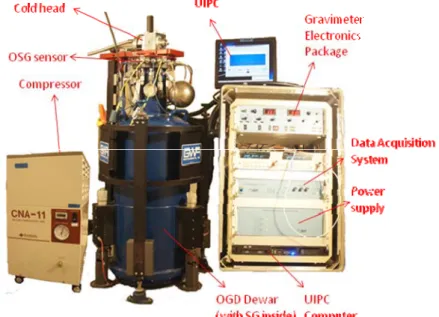
Fig. 1-2 Layout of NGDS, T48 is installed at B2 ... 3 Fig. 2-1 T48 at LOGG, showing the coldhead, integrated electronics with digital data

acquisition system (DDAS) and user interface PC (UIPC) software. ... 7

Fig. 2-2 A cross section scheme of the T48 sensor (GWR, 2011) ... 8 Fig. 2-3 Refrigeration system of Sumitomo CNA-11 helium compressor, and

Sumitomo RDK-101E coldhead of T48 ... 10

Fig. 2-4 integrated electronics and data acquisition system of T48 ... 11 Fig. 2-5 The UIPC main page, showing 1-s (top panel) and 60-s real-time (grav1),

filtered gravity (grav2) and barometer data (baro-1), GPS status, liquid helium status, DAC status and alarm status. ... 12

Fig. 2-6 Principle of AG measurement by laser to detect distance and rubidium to

detect time (FG5 Manual, 2006) ... 13

Fig. 2-7 The schematic of a FG5 system. (FG5Manual, 2006) ... 15 Fig. 2-8 Measuring gravity values at different heights for gradient determination ... 18 Fig. 2-9 Gravity gradients and standard errors (vertical bars), and the trends of

gradient ... 19

Fig. 2-10 Gravity values (relative to the mean of all measurements) and standard

errors (vertical bars) at pillar B1 observed by the FG5 #224 and #231 gravimeters ... 22

Fig. 3-1 The raw data before (top) and after (bottom) removing discontinuties and

disturbances. ... 24

Fig. 3-2 Filter response functions of the low-pass (left) and high-pass (right) used in

(9)

Fig. 3-3 Gravity values based on DDW (Dehant et al., 1999) solid earth model from

July 1, 2009 to September 30, 2009 ... 26

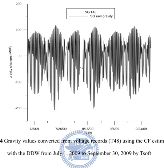
Fig. 3-4 Gravity values converted from voltage records (T48) using the CF estimated

with the DDW from July 1, 2009 to September 30, 2009 by Tsoft ... 27

Fig. 3-5 Four cases of estimating CF of T48 by FG5 #231 ... 29 Fig. 3-6 Signal (top) and residual (bottom) from T48 during liquid helium loss. The

residual gravity shows a clear drop associated with the helium loss. ... 32

Fig. 3-7 Procedure of solid earth tide from (left), procedure of ocean tide loading

(middle), procedure of observed (right) from T48 ... 33

Fig. 3-8 Sub-seismic noise levels of residual gravity at HS station, compared with

other SG stations (the names are defined on the GGP web page) ... 34

Fig. 4-1 Tidal spectra of raw gravity records in five years were recorded by T48. Two

clusters are present at the semi-diurnal and diurnal wave bands. Tides with periods shorter than the period of M3 are not shown here. ... 35

Fig. 4-2 Comparison the raw gravity records and observed models of T48 and T49 in

January 1, 2009. ... 40

Fig. 4-3 Difference amplitudes from T48 and T49 (T49 minus T48)... 40 Fig. 4-4 Difference phases from T48 and T49 (T49 minus T48). ... 41 Fig. 4-5 Amplitudes of ocean tide from tide gauge records at the Hsinchu Harbor (8.6

km to HS), and amplitudes of ocean tide loading from the SG gravity measurements at HS ... 44

Fig. 5-1 Raw atmospheric pressure over 4/2006-12/2010 (left) and the distribution of

the atmospheric pressure (right) ... 51

Fig. 5-2 Spectra of SG gravity (Red) and atmospheric pressure (Blue) ... 51 Fig. 5-3 Observed residual gravity changes (by T48, without the solid earth tide and

(10)

April 2006. ... 55

Fig. 6-1 Geological settings around the NGDS and distributions of GPS and tide

gauge stations. The meanings of the formations are explained by documents in the Central Geological Survey of Taiwan. ... 58

Fig. 6-2 A cross-section along the alluvium north of HS showing layers with shallow

and deep groundwater. Deep groundwater takes time to fill and will delay groundwater-induced gravity change. The sampling points A, B, C, D and E are shown in Fig. 6-1 ... 58

Fig. 6-3 The variations of coordinate are at the HCHM, TCMS, SHJU and HSIN

permanent GPS stations. The numbers in the figure panels are linear rate of

displacements from LSQ fits to the coordinate variations. ... 60

Fig. 6-4 Absolute gravity sites in Taiwan established by MOI ... 62 Fig. 7-1 Comparison of SG and FG5 measurements are from 2006-2011. The FG5

gravimeter #228 is from France while #224 and #231 are from Taiwan. ... 64

Fig. 7-2 AG sites in the project AGTO (circle) and GPS sites (star) ... 66 Fig. 7-3 The elevation of AG sites in the project AGTO, AG3 and AG6 are located at

the mid-slope of a mountain ... 67

Fig. 7-4 Formosat-2 images of AG3 and AG6 before and after Morakot ... 67 Fig. 7-5 Accumulation of soil and rock in the riverbed near AG6 due to Morakot

(brown), and the original riverbed (green) ... 68

Fig. 7-6 Gravity changes relative to observations in 2006 at AGTO sites (each curve

represents a year) ... 70

Fig. 7-7 Gravity changes relative to the observations in 2006 at the AGTO sites (each

curve represents a site) ... 70

Fig. 7-8 Absolute gravity values and rate at DSIG ... 75 Fig. 7-9 Absolute gravity values and rate at FLNG ... 75

(11)

Fig. 7-10 Absolute gravity values and rate at HCHG ... 75

Fig. 7-11 Absolute gravity values and rate at JSIG ... 75

Fig. 7-12 Absolute gravity values and rate at KDNG ... 76

Fig. 7-13 Absolute gravity values and rate at LYUG ... 76

Fig. 7-14 Absolute gravity values and rate at PKGG ... 76

Fig. 7-15 Absolute gravity values and rate at SMLG ... 76

Fig. 7-16 Absolute gravity values and rate at TAES ... 77

Fig. 7-17 Absolute gravity values and rate at TCHG ... 77

Fig. 7-18 Absolute gravity values and rate at TLGG ... 77

Fig. 7-19 Absolute gravity rate of WFSG station ... 77

Fig. 7-20 Absolute gravity rate of YHEG station ... 78

Fig. 7-21 Absolute gravity values and rate at YLIG ... 78

Fig. 7-22 Absolute gravity values and rate at YMSG ... 78

Fig. 7-23 Two-dimensional (lateral) distribution of gravity rates interpolated from the rates at AG sites ... 79

Fig.7-24 Horizontal displacement rates (arrows) and vertical displacement rates (color) from GPS. An arrow corresponds to a continuous GPS station... 79

Fig. 8-1 Weather sensor outputs during Typhoon Morakot (top) and SG gravity data in Hsinchu with and without atmospheric pressure effects. ... 81

Fig. 8-2 Weather sensor outputs during Typhoon Kalmaegi (top) and SG gravity data in Hsinchu with and without atmospheric pressure effects. ... 82

Fig. 8-3 A plane view (left) and perspective view of the 3-D atmospheric pressure model for Morakot ... 87

Fig. 8-4 A plane view (left) and perspective view of the 3-D atmospheric pressure model for Kalmaegi ... 88

(12)

contributions ... 88

Fig. 8-6 Co-seismic gravity change, given as a jump (step function) in the SG gravity

records at HS, due to the earthquake on September 6. ... 90

Fig. 8-7 Magnitude 9.0 – near the east coast of Honshu, Japan earthquake on March

(13)

Chapter 1 Introduction

1.1 Background

Taiwan, like many other regions in the western Pacific, is prone to attack from such hazards as landslide, typhoon and earthquake, which may create mass changes and in turn gravity changes. Such gravity changes are usually over a small area, and cannot be sensed by the gravity sensor of a satellite gravity mission such as GRACE, but might be detected by a highly-sensitive, ground-based gravimeter such as SG. In April 2006, two single-sphere observatory SGs (OSGs), serial numbers T48 and T49, were installed at tunnel B of Mt. 18-Peak in Hsinchu City, Taiwan. At the same time, two absolute gravimeters (AGs), serial numbers 224 and 231, were introduced in Taiwan. All the gravimeters belong to Ministry of the Interior (MOI) and setup in tunnels of the national gravity datum service (NGDS).

T48 and T49 were manufactured by GWR and have a nominal sensitivity of one ngal and a stability of 6 μgal year-1 or better (1 ngal = 10-11 m s-2). The HS SG station is now included in the SG network of GGP (Fig. 1-1). The GGP’s objective in the global geodetic observing system (GGOS) is to provide high quality SG data for geodynamic research. Most of the AG measurements collected with the two AGs (FG5 #224 and FG5 #231) are carried out by the laboratory of geodesy and geodynamics (LOGG, http://www.logg.org.tw/, Fig. 1-2). The latitude, longitude and elevation of LOGG are 24.79258 ºN, 120.98554 ºE and 87.6 m, respectively. LOGG is about 8.6 km from the Taiwan Strait, where the average depth is 80 m. Here the ocean tide amplitude and phase change rapidly (Jan et al., 2004).

HS is the closest station to the Tropic of Cancer in GGP and will be most sensitive to gravity change due to the motion of the earth’s inner-core in the summer solstice, making HS the best for testing the universality of free fall (Shiomi, 2006). Real-time

(14)

data of typhoons, earthquakes and continuous GPS observations around Taiwan, accessible at the central weather bureau (CWB, http://www.cwb.gov.tw/ ) of Taiwan, are used in connection to SG. The introduction of these gravimeters motivates this study, which will focus on the regional characteristics of Taiwan. Specifically, this study will emphasize gravity datum establishment, geodynamics and atmospheric events.

GPS is an important tool to aid the interpretation of gravity data and it will be also covered in this study. The study will monitor and analyze the mechanisms of gravity changes and GPS changes from 2006 to 2011. The events of typhoons and earthquakes affect gravity changes and may contribute most to gravity and geometric changes in some cases. They will be also investigated using SG, AG and GPS in this dissertation.

Fig. 1-1 Current and planned SG stations in the world, squares represent the new

stations, circles the current stations, diamonds the planned stations (Described in the ggpnews20, 2010)

(15)

Fig. 1-2 Layout of NGDS, T48 is installed at B2

1.2 Literature Review

There are many phenomena that cause environmental changes in Taiwan. This study uses gravimeters to monitor selected phenomena. Because of this, we need a gravity datum as the basis for analyzing the mechanisms of such phenomena. SG is highly sensitive to gravity changes due to solid earth tide, ocean tide loading, atmosphere, groundwater, soil moisture, tilt variation and other environmental changes (e.g. Warburton and Goodkind, 1977; Crossley et al., 1995; Dal Moro and Zadro, 1998; Neumeyer et al., 2004; Boy and Hinderer, 2006). It is necessary to explain the physical significance of SG and to identify the standard operating procedure (SOP) for SG data processing. After removing data noises, including spikes, gaps and steps of SG, we use the parallel observations of AG and SG values for data comparison and calibration (Van Ruymbecke, 1989; Richter et al., 1995; Falk et al., 2001). Currently, the most commonly used technique for calibration of SG record is based on parallel observations of SG and AG (Sato et al., 1996; Francis et al., 1998; Imanish et al., 2002). If AG is not available, the CF of SG is usually determined by comparison between the

(16)

theoretical solid earth tide and SG raw measurements (voltage). The nominal drifting rate of SG is 6 μgal year-1 claimed by GWR instrument (Warburton and Brinton 1995), but the drifting rate could vary from one SG to another.

With SG, it is possible identify gravity changes of non-tectonic origins, such as those due to typhoons and earthquakes (Imanishi et al., 2002). The gravity-atmosphere admittances for various atmospheric conditions in typhoons will vary and is a potential application of SG (Kim et al., 2011). The impact of typhoon-generated gravity changes could be large during the developing stage than during the mature and decaying stages of the typhoon (Kim et al., 2011). About 90% of the atmospheric effects were attributed to local atmospheric variations within 50 km of the station (Mukai et al., 1995). Selected co-seismic gravity perturbations have been detected and analyzed using SG to demonstrate the sensitivity of SG, and the SG results have been compared with those obtained by seismometers (Imanishi et al., 2004; Hwang et al., 2009; Kim et al., 2009; Nawa et al., 2009). In addition, AG and continuous GPS measurements have been used to study mass transfer and vertical movement due to mountain building (Segall and Davis, 1997; Jacob et al., 2008).

1.3 Outline of dissertation

This dissertation is organized into 9 chapters. Chapter 2 is to present the principles of SG and AG, including an in-depth introduction of instruments, specifications and software. Chapter 3 describes data processing of SG, including filtering, CF, modeling the solid earth tide and ocean tide loading. Chapter 4 describes the effect of ocean tide loading, tidal analysis, and comparison with theoretical solid earth tide. Chapter 5 shows the environment effects on gravity observations. Chapter 6 presents the geological settings around the NGDS, it is the key work for establishing an AG reference and data preparation for the GGP. Chapter 7 shows the result from gravity

(17)

observations of the project “AGTO” in southern Taiwan, jointly conducted by France and Taiwan. The motivation of AGTO is to see mass changes due to middle-to-long term tectonic motion from repeated gravimetric and continual GPS measurements. The gravity and vertical trends of 25 AG stations and 313 permanent GPS stations will be presented. Chapter 8 presents an extensive discussion on global atmospheric and local atmospheric effects on gravity. The gravity effects from Typhoon Kalmaegi and Morakot are described in detail in this chapter. Finally, a summary, conclusions and suggestions are presented in the final chapter.

(18)

Chapter 2 Principles of superconducting gravimeters and

absolute gravimeters at LOGG

2.1Superconducting gravimeter

2.1.1 Introduction

The following discussion is largely based on the existing literature and internet information of SG (i.e., http://www.gwrinstruments.com). Since every SG or AG gravimeter is unique when it is manufactured, the purpose of this chapter is to present information that is mostly exclusive to the SG and AG gravimeters at LOGG. In the dewar of T48 (Fig. 2-1), there is a spherical proof mass levitated by the forces from a magnetic field generated by a pair of superconducting coils. Continued currents generate the magnetic field that is superconducting below a temperature of 9.3 K in two niobium coils (GWR, 2011). There are magnet coils without resistive loss and decay in time between the two niobium coils. Compared to a relative gravimeter using metal spring, the sensor of magnet force gradient of SG can detect a very weak signal. Small changes in gravity produce large displacements of the proof mass. The displacement transducers set around the proof mass to detect the weak gradient in the stable magnetic field. T48 and T49 at LOGG have the features described above, and can contribute to applications as follows:

(1) Resolving density of mass change related to elevation change measured by GPS. (2) Continuous gravity monitoring of geophysical phenomena such as solid earth tide,

ocean tide loading, atmospheric loading, hydrology, and Earth rotation.

(3) Validation of satellite gravity observations from CHAMP, GRACE and GOCE. (4) Real-time monitoring of volcanoes.

(5) Monitoring long-term crustal motion and sea level anomaly. (6) Calibrating AG measurements.

(19)

(7) Establishing a high-accuracy gravity reference station (together with AG).

Fig. 2-1 T48 at LOGG, showing the coldhead, integrated electronics with digital data

acquisition system (DDAS) and user interface PC (UIPC) software.

2.1.2 Observatory SG (OSG) sensor

An OSG is equipped with all the necessary units designed to store the electronic signals, and maintain the SG automatically at low temperature (Fig. 2-1). The analog controller is integrated with the DDAS and generates gravity output in digital format. The gravimeter sensing unit (GSU, Fig. 2-2) is built around a 2.5 cm diameter spherical proof mass which is made in a stable magnetic field and different from a conventional gravimeter. Since the sphere is superconducting with perfect diamagnetism, the surface currents on the sphere are not affected by any magnetic fields from GSU’s interior. The interaction is between the applied magnetic field and the surface currents of sphere which produce the levitation force.

A superconducting magnetic shield is built around GSU to exclude the effects from the external magnetic field. The thermal shield sensor is put around the vacuum chamber where and temperature is stable in a few K. This sensor makes the gravity unit

(20)

insensitive to environmental effects such as changes in external humidity, temperature and atmospheric pressure. The OSG sensor specifications of T48 and T49 are as follows (GWR, 2011):

(1) Precision: 0.1 to 0.3 μgal Hz-1/2

(2) Drift: Typically less than 6 μgal year-1 after the initial 6 to 12 months of stabilization period

(3) Calibrate: The manufacture, GWR, does not provide with calibration data of the GSU sensor. Users generally either perform a coarse calibration by parallel observing with AG and SG or fitting the observed gravity signal to the theoretical model of solid earth tide.

(4) Stable Calibration Factor: Comparing the OSG signal with models of solid earth tide, the scale factor is considered to be constant with variations smaller than 0.01% over several years.

(21)

2.1.3 Refrigeration System

The super-insulated dewar of a SG is operated in the 4 K cryogenic refrigeration system. This design removes the need to refill the dewar with liquid helium after the system is cooled down. When unrefrigerated, the loss rate of liquid helium is less than 5% per day and has chance to refill the dewar in 20 days. This capacity offers sufficient helium reserves so that the instrument can continue to operate under power failures or refrigeration maintenance.

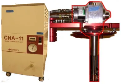
The helium refrigeration system is an independent system separated from the liquid helium dewar. The relative pressure of helium gas in the dewar is controlled in a range from 0 to 0.5 PSI, but the refrigeration system needs to operate at 350 PSI. These two helium gas circuits do not contact with each other. The refrigeration system consists of a helium compressor, coldhead (Fig. 2-3), vibratile diaphragm and flexible interconnected hoses. The application of the 4 K refrigeration system allows a much longer continuous interval of data collection. Noise related to the liquid helium is small and there are only occasional disturbances due to scheduled service of the coldhead. In summary, the refrigeration system specifications of T48 and T49 are as follows (GWR, 2011):

(1) Capacity: 35 liters

(2) Dimensions: 42 cm diameter x 114 cm high

(3) Total height installed on support feet: dewar is 116cm, dewar with coldhead is 130cm

(4) Minimum height required to transfer liquid helium (with standard equipment): 180 cm

(5) Hold time between refills (un-refrigerated): 20 days minimum (6) Weight of dewar with GSU installed: 60 kg

(22)

Fig. 2-3 Refrigeration system of Sumitomo CNA-11 helium compressor, and

Sumitomo RDK-101E coldhead of T48

2.1.4 Integrated electronics

The integrated electronics and data acquisition package (IEDP, Fig. 2-4) are used to control and monitor the SG, as well as provide SG log data. The sub units of IEDP are listed as follows (GWR, 2011):

(1) Gravimeter electronics package(GEP-3) 1. Gravimeter control electronics 2. Tilt control electronics

3. Temperature control electronics 4. Auxiliary electronics

5. GEP-3 remote control card, A/D converter and Setup circuitry (2) Data acquisition system (DDAS-3)

1. Data acquisition controller (DAC) 2. UIPC software

3. High resolution 7½ digit resample of “Agilent 34420A nano-volt meter” 4. Trimble GPS receiver

(23)

5. Optical isolators and lightening arrestors for digital data 6. DDIG-3 - OSG dual digitizer package

(3) DPS-4 - Current supply for initializing levitation magnets (4) VOTS-3 - Voltage transfer standard package

(5) TREE-3 - Temperature regulated electronics enclosure

(6) PRE-5 - Paroscientific met-3 meteorological measurement system

Fig. 2-4 integrated electronics and data acquisition system of T48

2.1.5 User interface PC software

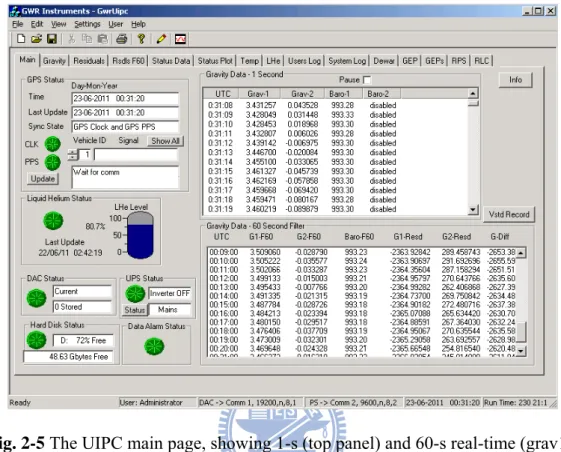
The user interface PC (UIPC) is part of the DDAS-3 data acquisition system, and contains a custom software program. The operator has the full right to control the SG functions, including the specification of atmospheric instrument, operation procedures, data logging and archiving. The UIPC software for all data channels is displayed in graphical and archiving in the monthly data. The operator needs to enter notes when the system has changed. A general alarm system is automatic described to trigger when any channels exceed normal limits and email notification to the operator in a number of ways. We can write the automated FTP routine in the operation system to

(24)

automatically upload data to different archival sites on a daily basis. The graphical user interface (GUI) of configurations is in Fig. 2-5.

Fig. 2-5 The UIPC main page, showing 1-s (top panel) and 60-s real-time (grav1),

filtered gravity (grav2) and barometer data (baro-1), GPS status, liquid helium status, DAC status and alarm status.

2.2Absolute gravimeter

2.2.1 Introduction

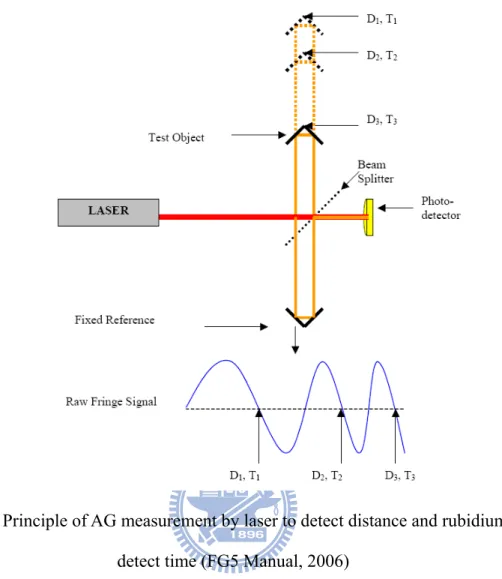
An AG determines the vertical acceleration based on the measurements of travelling distance and time of a free falling corner cube. It provides the direct measurement of absolute gravity. As shown in Fig. 2-6, the optical fringes go through zero and the precise time are recorded by an atomic clock. A least-square (LSQ) fit to the time and distance pairs is used to determine the gravity.

(25)

Fig. 2-6 Principle of AG measurement by laser to detect distance and rubidium to

detect time (FG5 Manual, 2006)

The following example shows how an absolute gravity value is measured by an absolute gravimeter. The traveling distance of a free-fall test mass in the dropping chamber is expressed as (FG5, 2006) 2 0 0 2 1 i i i x v t gt x = + + _(2-1)

where x0 is the origin height, ti is the travel time, v0 is the initial velocity, and g

is the gravity. With three distance measurements, x1 =D1−D0 , x2 =D2−D0 ,

0 3

3 D D

(26)

2 3 3 0 3 2 2 2 0 2 2 1 1 0 1 2 1 2 1 2 1 gt t v x gt t v x gt t v x + = + = + = (2-2)

By setting S1 = x2 −x1, S2 = x3 −x1 , t1 =T2 −T1 , t2 =T3 −T1 , and removing v0,

we have 1 2 1 1 2 2 ₎ ( 2 t t t S t S g − − = _(2-3)

where g is the absolute gravity value. The accuracy of the distance measurements by laser interferometer is about 10-8 ms-2 and the accuracy of the time measurement by a rubidium clock is 10-13 s. These accuracies combine to yield an accuracy of μgal for a gravity measurement.

2.2.2 Specifications of FG5

At LOGG, there are two FG5 gravimeters with serial numbers are 224 and 231. Each of the gravimeters consists of (Fig. 2-7):

(1) Dropping (or Vacuum) Chamber (2) Interferometer Base

(3) Superspring (4) Laser

(5) System Controller (6) Electronics.

(27)

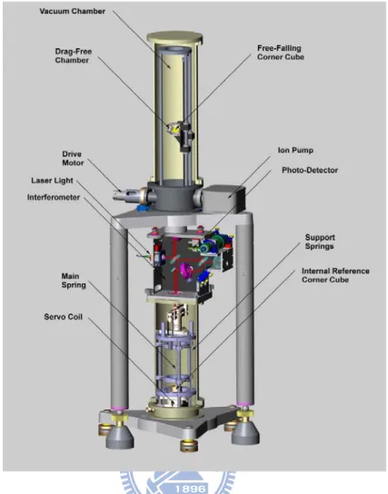
Fig. 2-7 The schematic of a FG5 system. (FG5Manual, 2006)

The system specifications of FG5 are as follows: (1) Power: 100-240 V AV

(2) Weight

1. Interferometer Base & Laser: 20 kg 2. Dropper: 25 kg 3. Superspring: 20 kg 4. Turbo Pump: 15 kg 5. Dropper Tripod: 20 kg 6. Superspring Tripod: 12 kg 7. Electronic Rack: 15 kg Total: 127 kg

(28)

(3) Transit case dimensions

1. Interferometer base (IB) & Laser: 64 x 56 x 38 (cm) 2. Dropper: 64 x 38 x 80 (cm) 3. Superspring: 31 x 30 x 57 (cm) 4. Turbo pump: 37 x 37 x 47 (cm) 5. Dropper tripod: 77 x 56 x 28 (cm) 6. Superspring tripod: 64 x 56 x 38 (cm) 7. Electronic rack: 64 x 56 x 38 (cm) 8. Computer: 38 x 32 x 7 (cm) (4) Operating temperature: 15-30 ℃

The corner cube is allowed to free-fall inside the vacuum dropping chamber. Interferometer base is used to monitor the position of the corner cube which is falling in the dropping chamber. The superspring is an active long-period isolation device used to provide an inertial reference for the gravity measurement. The computer allows the user to operate user interface, control the system, change the processing of data, and stores the results. The system provides high accuracy timing for the measurement which is necessary when doing the high precision absolute gravimetry.

2.2.3 Gravity gradient for gravity reduction

Gravity gradient is needed to reduce the height effect on gravity observations. For example, a raw FG5 observation may refer to a reference point along the dropping chamber and it may be reduced to a gravity value at the pillar marker or at a desired height for later applications. The relationship between vertical position z and gravity

(29)

z g g dt z d γ + = 2 2 (2-4)

where t is traveling time of the test mass, g and _{g are gravity and gravity gradient.}_γ The traveling distance is a function of time, velocity and gravity:

) 2 1 ( ) 6 ( ) 12 ( 2 1 ) ( 2 3 4 2 g t x t g t v t g t g t z = + γ + + γ + + γ _(2-5)

where x and v are the initial position and velocity. In this study, a GRAVITON-EG gravimeter is used to measure gravity gradients.

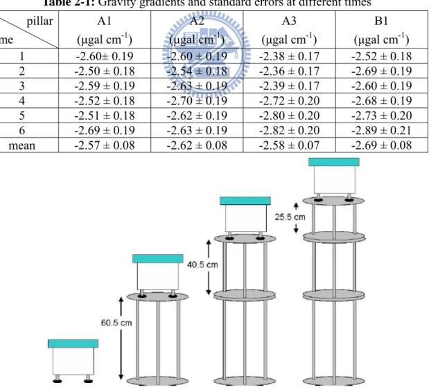
A GRAVITON-EG is a fully automated and portable gravimeter for determination of relative gravity. For gravity gradient determination, a GRAVITON-EG is set up at different heights (Fig. 2-8), where the gravity values are measured. The ratio between the differences in gravity and height is the gravity gradient. The measured gravity gradients at pillar A1, A2, A3 and B1 of LOGG (Fig. 1-2) are listed in Table 2-1 and are used for gradient reductions for AG measurements at LOGG. Six campaigns of gravity gradient measurements are illustrated in Fig. 2-9. We find that gravity gradient measurements at A3 are more stable than those at A1, A2 and B1. Because a gradient is computed as the ratio:

1 2 1 2 h h g g g_r − − = _(2-6)

where g₂, g1are the measured gravity values at different height h2, h1. We can

(30)

1 2 2 2 2 1 h h g g gr − + = σ σ σ _(2-7) where r g

σ is the standard error of each site. The gravity gradients at A1, A2, A3 and B1 range from -2.69 to -2.57 μgal cm-1. Such variations are due to different accuracies of the GRAVITON-EG that are largely results of environmental noises. For example, a large rainfall, a strong wind and a busy traffic will lead to large gravity perturbations that result in a degraded gravity measuring accuracy. The mean values in Table 2-1 are used for gravity reduction.

Table 2-1: Gravity gradients and standard errors at different times

pillar time A1 (μgal cm-1) A2 (μgal cm-1) A3 (μgal cm-1) B1 (μgal cm-1) 1 -2.60± 0.19 -2.60 ± 0.19 -2.38 ± 0.17 -2.52 ± 0.18 2 -2.50 ± 0.18 -2.54 ± 0.18 -2.36 ± 0.17 -2.69 ± 0.19 3 -2.59 ± 0.19 -2.63 ± 0.19 -2.39 ± 0.17 -2.60 ± 0.19 4 -2.52 ± 0.18 -2.70 ± 0.19 -2.72 ± 0.20 -2.68 ± 0.19 5 -2.51 ± 0.18 -2.62 ± 0.19 -2.80 ± 0.20 -2.73 ± 0.20 6 -2.69 ± 0.19 -2.63 ± 0.19 -2.82 ± 0.20 -2.89 ± 0.21 mean -2.57 ± 0.08 -2.62 ± 0.08 -2.58 ± 0.07 -2.69 ± 0.08

(31)

1 2 3 4 5 6 campaign -3.2 -3 -2.8 -2.6 -2.4 -2.2 -2 g rav ity g radi e n t ( ga l c m -1)

LOGG gravity gradient A1 Fit 1: A1 A2 Fit 1: A2 A3 Fit 1: A3 B1 Fit 1: B1

Fig. 2-9 Gravity gradients and standard errors (vertical bars), and the trends of

(32)

2.2.4 Quality assessment of AG measurement

The estimated precision of an AG gravity value is based on the repeated measurements from the total drops, plus the standard errors (uncertainties). First, the standard error of a single gravity measurement is estimated from repeated measurement at the same location as :

1 ) ( 1 2 − − =

∑

= n g g n i i σ _(2-8)

where σ is the standard error, n is the number of measurements, g_i is the

measurement, and g is the average of the measurements. The standard error of the mean value is

n g

σ

σ = _(2-9)

In addition to measurement errors, the uncertainties in models include the environmental gravity effects. A corrected mean gravity is:

∑

= − = ′ k i i C g g 1 (2-10)

where C_i are the environmental gravity effects. If the gravity effects are uncorrelated,

(33)

∑

= ′ = + k i C g g i 1 2 2 _σ σ σ _(2-11) where 2 i C

σ are the error variance of the model corrections. The g software can

estimate the total uncertainties based on repeat measurements and the built-in correction models.

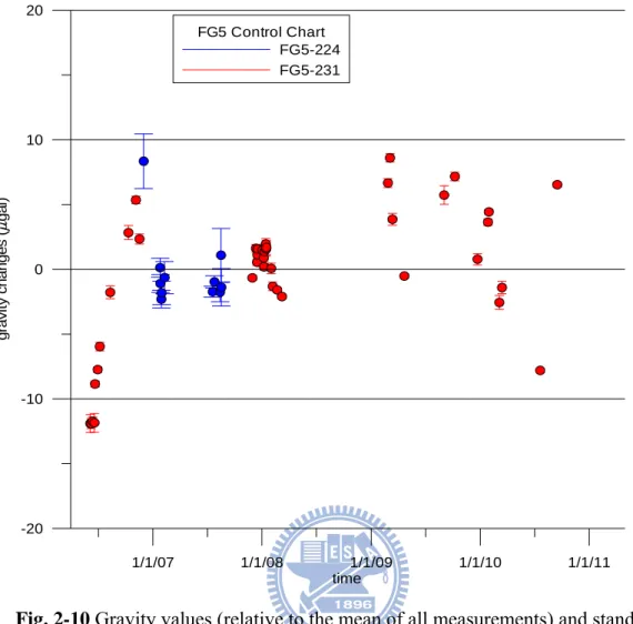
FG5 #231 has been set up at LOGG to measure gravity values on B1 and T48 is set up on B2. More than 70 AG observation records have been collected on B1 from 2006 to 2011. The gravity gradient of B1 is -2.69 μgal cm-1 (see Table 2-1) and it is used for the reduction of raw FG5 records to ground values. The mean gravity from 2006 to 2011 is 978,901,463 μgal. Fig. 2-10 shows the gravity values with standard errors. The total standard errors (uncertainties) range from 0.14 to 0.53 μgal, and such variations in the total standard errors are mostly due to background noises/vibrations that affect the laser frequency.

Table2-2: Absolute gravity measurements and result on B1 from FG5 #231 in 2010

Time Drop number

Gravity (μgal) Standard

error of mean (μgal) Total uncertainty (μgal) January 27, 2010 2977 978,901,199 0.25 2.06 January 31, 2010 21976 978,901,199 0.16 2.03 March 6, 2010 2591 978,901,192 0.53 2.08 March 15, 2010 3786 978,901,194 0.48 2.08 July 23, 2010 28310 978,901,187 0.14 2.03 September 16, 2010 2989 978,901,202 0.18 2.02

(34)

1/1/07 1/1/08 1/1/09 1/1/10 1/1/11 time FG5 Control Chart FG5-224 FG5-231 -20 -10 0 10 20 g ra v it y change s ( ga l)

Fig. 2-10 Gravity values (relative to the mean of all measurements) and standard

(35)

Chapter 3 Processing SG data

3.1 Filtering and decimation of raw SG data

The gravity records (measured in voltage) at the 1-s (one-second) interval from T48 have been recorded from April 1, 2006 to present. The data contains noises and signals of various origins such as earthquakes or other disturbances caused by human interferences. The raw data should be screened and repaired before use. In this study, the spikes and other disturbances were removed using TSoft software, which is the standard software provided by the International Center for Earth Tides (ICET, http://www.astro.oma.be/ICET/ ) for SG data processing. Fig. 3-1 illustrates the time series before and after fixing a discontinuity in the data record. The discontinuity is like a cycle slip in GPS phase data. The discontinuity removal is based on the comparison between the predicted and observed values after the discontinuity. This discontinuity fixing is very important to an un-interrupted, long-term record of SG observations that are used to validate/calibrate satellite gravity observations from missions like GRACE. In particular, it is only possible to obtain reliable inter-annual change of gravity from SG with SG records without step functions (discontinuities) in the records.

In case of data loss due to instrument or helium problems, the data gaps are filled by theoretical values from the Dehant-Defraigne-Wahr (DDW) solid earth model. The data are then LSQ fitted to generate records at the 1-m (one-minute) and 1-h (one-hour) intervals using a filtering procedure, which, together with the raw 1-m data, are uploaded to GGP. The 1-m and 1-h data are used for subsequent processes and analyses. TSoft can accept different sample rates, which are specified in two steps. The first step is to define the new sample rate and change the interpolation type. There are three types of interpolator in Tsoft: linear, cubic and cumulative interpolators. The second

(36)

step is to choose the LSQ-filter types. The LSQ-filter removes outliers and performs filtering. It can also decimate 1-s data (the smallest sampling interval of SG) to a larger interval (e.g., one-minute or one-hour). Before data decimation, filtering must be applied to the raw data to remove aliasing at a coarse (than 1-s) interval. The LSQ-filter in TSoft includes a low-pass and high-pass filter. A filter consists of two parameters: the cut-off frequency or central frequency f0, and the band width fw (see also Fig. 3-2). The cutoff frequency is the frequency beyond which the signal components are truncated to zero. In fact, filtering and re-sampling of the raw gravity records are made simultaneously. If the raw data contain discontinuity, gap and spike, Tsoft will first remove them and then performs filtering and re-sampling.

5/12/08 5/22/08 6/1/08 6/11/08 -12 -8 -4 0 4 8 g ravi ty ch an ge s (v olt ag e) SG T48 fixed 5/12/08 5/22/08 6/1/08 6/11/08 date -4 0 4 8 12 gr av ity c h an ge s (v olt ag e) SG T48 raw

Fig. 3-1 The raw data before (top) and after (bottom) removing discontinuties and

(37)

Fig. 3-2 Filter response functions of the low-pass (left) and high-pass (right) used in

the LSQ filters of TSoft

3.2 Calibration factor

3.2.1 Estimation of calibration factor using the DDW model gravity

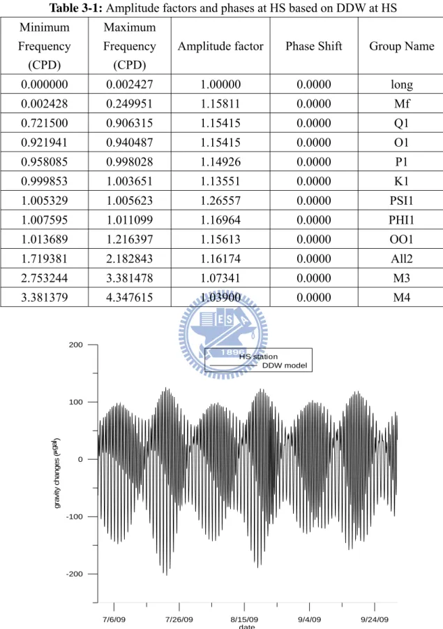
The CF of a SG is a number that converts a voltage measurement from SG to a gravity measurement. A method to estimate CF is by comparing gravity values from a solid earth tide model and voltage records of a SG. In this study, first we use TSoft to generate theoretical gravity values using the DDW solid earth tide model (Dehant et al., 1999) at a given location. By specifying the latitude of a given location, DDW may yield the theoretical amplitude factors and phases for various tidal components, which are used to compute theoretical gravity values. The modeled gravity values are then compared with the SG records (in voltage) to determine the CF of the SG gravimeter that generates the voltage records.

The amplitude factors and phases at selected frequency ranges based on the DDW solid earth tide at HS are listed in Table 3-1. Fig. 3-3 shows the theoretical gravity values from July 1, 2009 to September 30, 2009, which shows dominating variations at the semi-diurnal and diurnal bands. Fig. 3-4 shows the gravity values from the voltage records multiplied by the CF estimated. This method of CF estimation is a standard method employed at SG stations without parallel AG and SG measurements.

(38)

Table 3-1: Amplitude factors and phases at HS based on DDW at HS Minimum Frequency (CPD) Maximum Frequency (CPD)

Amplitude factor Phase Shift Group Name

0.000000 0.002427 1.00000 0.0000 long 0.002428 0.249951 1.15811 0.0000 Mf 0.721500 0.906315 1.15415 0.0000 Q1 0.921941 0.940487 1.15415 0.0000 O1 0.958085 0.998028 1.14926 0.0000 P1 0.999853 1.003651 1.13551 0.0000 K1 1.005329 1.005623 1.26557 0.0000 PSI1 1.007595 1.011099 1.16964 0.0000 PHI1 1.013689 1.216397 1.15613 0.0000 OO1 1.719381 2.182843 1.16174 0.0000 All2 2.753244 3.381478 1.07341 0.0000 M3 3.381379 4.347615 1.03900 0.0000 M4 7/6/09 7/26/09 8/15/09 9/4/09 9/24/09 date -200 -100 0 100 200 g ra v it y chan ge s ( ga l ) HS station DDW model

Fig. 3-3 Gravity values based on DDW (Dehant et al., 1999) solid earth model from

(39)

7/6/09 7/26/09 8/15/09 9/4/09 9/24/09 date -200 -100 0 100 200 grav it y c h a n g e s ( ga l ) SG T48 SG raw gravity

Fig. 3-4 Gravity values converted from voltage records (T48) using the CF estimated

with the DDW from July 1, 2009 to September 30, 2009 by Tsoft

3.2.2 Calibration factor from parallel SG and AG gravity observations

If an AG is available at a SG station, the CF of the SG is estimated using parallel observations of SG and AG. In this study, we also use AG to estimate the CF of T48 and T49 at HS. A preliminary result for T48 was reported in Hwang et al. (2009). This method has been demonstrated in various studies (e.g., Francis et al., 1998; Imanishi et al., 2002; and Tamura et al., 2005). In fact, the CF and the drifting rate of a SG are two crucial parameters that must be taken into account when using the SG data at HS.

The CF estimation in the following description will provide useful information to users of the HS SG data. Because T48 contributes data to GGP, we present a detailed result of estimating the CF of T48 and T49 below. T48 records used for CF estimation contain major jumps of up to 1000 μgal due to helium re-filling problems. Therefore,

(40)

careful treatments of the raw data must be made before computing CF. We determine an optimal CF of T48 using parallel observations of T48 and a FG5 #231 given in Table 3-2. The pillars for T48 and FG5 are separated by about 1 meter. In total, 17 sessions of parallel observations were collected in summary of first phase. The following model is adopted for the determination of the CF:

) ( ) ( ) (t fV t b s t g = _c + − (3-1)

where f_c is the CF, b is an offset, s is the drifting rate of T48, g and V are

records from FG5 and T48 (or T49), respectively. Given the observations ( g and V ), the standard LSQ technique is used to compute f_c and b . FG5 and SG sense the

same gravity effects of solid earth tide and ocean tide, as well as any other time-varying gravity effects, to produce gravity variations, which are exactly what we need for determining the CF. Before the LSQ solution, the outliers in the SG and FG5 data, which occur mostly during heavy rainfall, earthquakes and abrupt changes of air pressure due to typhoons, were removed. As an example, Fig. 3-5 shows the four cases of T48 and FG5 data for estimating the CF from the session of June 5, 2006 to February 2, 2008. The variation in the FG5 gravity records are mainly caused by solid earth tide and are almost linearly correlated with the SG records in voltage (correlation coefficient 0.953). The FG5 was not continuous measurement in case 1 due to an earthquake. The raw data whose difference with the filtered data exceed 3 times of standard error were removed. The FG5 #231 did not record continuous measurement in case 2, and again due to an earthquake. However, in case 3, the FG5 collected continuous measurement despite a big earthquake. In case 4, the FG5 records were continuous without earthquake interruptions. The residuals of FG5 observations from

(41)

the LSQ adjustment (raw FG5 gravity values minus fitted gravity values) roughly follow the normal distribution, suggesting that the linear model in Eq. (3-1) is adequate, and the estimated parameters in Table 3-2 are unbiased.

Fig. 3-5 Four cases of estimating CF of T48 by FG5 #231

In Table 3-2, there are three phases of T48 records and a new phase begins at the time of a major helium problem fixing. Phase 1 is from April 1, 2006 to March 15, 2008. Phase 2 is from March 16 to May 30, 2008. Phase 3 is from June 1, 2008 to present. The result in Table 3-2 shows different CF values are found in different measurement phases. This suggests that a major helium fixing will change the condition inside the dewar. In

(42)

theory, the position of the spherical proof mass will be moved after the major helium fixing, leading to a varying CF. Using all data in Table 3-2, we obtain a CF of -76.087 μgal voltage-1 for T48.

Table 3-2: Sessions of parallel superconducting (T48) and absolute (FG5) gravity

observations for determining the calibration factor of T48

FG5 #231 (GMT) drops CF (μgal voltage-1) offset1 Eq. (3-1) June 9-10, 2006 1614 -75.984 ±0.373 1701.521±1.220 June 13-14, 2006 1436 -76.350 ±0.360 1701.220±1.023 June 21-23, 2006 4318 -76.032 ±0.150 1701.265±0.439 June 30- July 2, 2006 4216 -76.621 ±0.242 1702.087±0.710 July 7-11, 2006 4004 -76.807 ±0.232 1701.646±0.675 October 11-12, 2006 1259 -77.383 ±0.433 1701.485±1.276 November 4-6, 2006 3344 -76.030 ±0.155 1698.591±0.461 November 17-18, 2006 2746 -75.622 ±0.349 1693.337±0.980 March 2-3, 2007 3087 -76.506 ±0.184 1685.009±0.546 March 4-7, 2007 3023 -76.499 ±0.417 1686.692±1.190 November 10-11, 2007 1722 -75.876 ±0.472 1679.035±1.409 November 30- December 3, 2007 7038 -75.838 ±0.366 1696.695±1.106 December 16-18, 2007 7758 -75.504 ±0.264 1695.724±0.731 January 2, 2008 2058 -75.465 ±0.566 1695.689±1.543 January 7-9, 2008 9938 -76.169 ±0.092 1697.120±0.270 February 6-7, 2008 2978 -75.407 ±0.353 1696.310±1.060 February 21-23, 2008 8901 -76.227 ±0.122 1697.254±0.263

Summary of first phase 42183 -76.087 ±0.067 1695.809±0.201

April 5-7, 2008 10375 -76.502 ±0.088 1440.698±0.274

Summary of second phase 10375 -76.502 ±0.088 1440.698±0.274

July 31- August 1, 2008 2449 -76.175 ±0.212 1440.698±0.274

January 15-20, 2009 12904 -75.617 ±0.212 1432.257±0.115

April 22-26, 2009 11580 -75.782 ±0.115 1444.486±0.129

Summary of third phase 27483 -75.547 ±0.094 1438.228±0.086

1 _{A mean}

(43)

3.3 Detided gravity

The gravity effect from the solid earth tide is a dominating signal in SG measurements. To assess gravity effects due to hydrological changes and other geodynamic phenomena, such a gravity effect should be removed from the raw SG gravity records. A gravity record without the solid earth tide effect is called detided gravity or residual gravity in this section. Both the raw and residual gravity records will contain the same step functions and other anomalous values, but the latter has a larger gravity magnitude. The step functions are removed manually in Tsfot from the raw data. After removing step functions from the raw data and calculating the residual, one should see whether the residual contains periodic signals. If periodic signals are present in the residual, it is likely that the fitted solid earth tide model is not sufficiently good. The anomalous gravity values such as the ones shown in Fig. 3-6, which are due to helium fixing, cannot be used to generate tidal parameters. Such a detided gravity (residual) can also be used to compute ocean tide loading gravity effects and other periodic gravity signals.

Depending on the purpose, there are different cases of detided gravity, which are defined and summarized in Fig. 3-7.

(1) Case 1: T48 solid earth tide

(1-1) The DDW gravity is removed from the corrected gravity to yield tide-free gravity.

(1-2) The difference between corrected gravity and tide-free is computed to obtain refined gravity.

(1-3) The refined gravity is used to compute amplitude factors and phases. (2) Case 2: T48 ocean tide loading

(2-1) The effects of atmospheric effect, ground water effect, soil moisture effect, and polar motion effect are removed from the corrected gravity (section

(44)

5.2).

(2-2) The result of gravity is used to compute ocean tide loading (3) Case 3: T48 observed tide

(3-1) The raw SG gravity is filtered, decimated, calibrated to yield corrected gravity.

(3-2) The corrected gravity is used to estimate all periodic signal components, which are included all environment effects.

2/16/09 3/8/09 3/28/09 4/17/09 date -30 -20 -10 0 10 g ra v it y chan ges ( ga l) SG T48 residual gravity 2/16/09 3/8/09 3/28/09 4/17/09 -200 -100 0 100 200 g ra v it y c han ges ( ga l) SG T48 raw gravity

Fig. 3-6 Signal (top) and residual (bottom) from T48 during liquid helium loss. The

(45)

detide remove DDW

model

SG gravity without solid earth tide

raw SG gravity remove SG gravity without solid earth tide

detide

raw SG gravity remove solid earth tide model

from SG remove atmospheric effect remove ground water effect remove soil moisture effect remove polar motion effect detide

Case 1 – T48 solid earth tidel Case 2 - T48 ocean tide loading Case 3 - SG T48 observed

SG T48 observed model SG T48 ocean tide loading SG T48 solid earth tide model

raw SG gravity raw SG gravity raw SG gravity raw SG gravity

Fig. 3-7 Procedure of solid earth tide from (left), procedure of ocean tide loading

(middle), procedure of observed (right) from T48

3.4 Sub-seismic noise levels of residual gravity from T48

Since the beginning of GGP in 1997, the number of SG stations has increased to 30 in 2011. SG has been used principally in tidal studies due to its high sensitivity and low drifting rate. But when searching for elusive signals, like the gravity variations associated with the translational mode of the inner core, stacking data of different sites is needed. Data from GGP allow the comparison of noise levels of different stations.

(46)

The noise level with the New Low Noise Model (NLNM, Peterson, 1993) is used as a reference model to give an estimation of the quality of a SG (Rosat and Hinderer, 2011). NLNM is a model that shows the lowest noise level of a seismometer. Here we compare the spectra of residual gravity from several continuously recording SG stations like HS, Bad Homburg (BH), Membach (MB), Canberra (CB), Medicina (MC), Sutherland (SU) and Strasbourg (ST) (Fig. 3-8).

We use a standard procedure to obtain the power spectral densities (PSDs) of residual gravity over a quiet time period in order to evaluate the combined instrument and site noise in the frequency band of 0.01 to 10 mHz at the selected SG stations. Fig. 3-8 shows the spectrum of the residual gravity from T48 measurements in June 2008, along with the spectrum implied by NLNM. At frequencies less than 0.03 mHz, the spectra of T48 exceed that of NLNM, suggesting that the SG records at HS yield noises that are larger than theoretical noise level of a seismometer. The PSD of HS is on average larger than those at other stations. This is mainly because the HS station is 8.6 km to the oceans, which creates high-frequency oscillations in the T48 observations.

Fig. 3-8 Sub-seismic noise levels of residual gravity at HS station, compared with

(47)

Chapter 4: Analyses of tidal parameters and ocean tide

loading gravity effects

4.1 Spectral analysis of SG gravity records

We use Tsoft to decimate the T48 records to the 1-h records for tidal analysis. Fig. 4-1 shows the spectrum of the raw SG gravity records. As expected, we observe the six leading tidal components of M2, K1, S2, O1, N2 and P1. Note that the distinct signal component labeled M3 in Fig. 4-1 at a frequency of about 2.9 cycle day-1, which is due to the M3 ocean tide modulated by the complex bathymetry and coastal lines around the Taiwan Strait. This shows that, as pointed out by Hinderer and Crossley (2004), and Boy et al. (2004), SG provides interesting and important data to study non-linear tides over such a shallow-water area as the Taiwan Strait.

Fig. 4-1 Tidal spectra of raw gravity records in five years were recorded by T48. Two

clusters are present at the semi-diurnal and diurnal wave bands. Tides with periods shorter than the period of M3 are not shown here.

(48)

4.2 Tidal analysis

Hourly data of SG are generally used to estimate the gravimetric solid earth tide. These measurements contain information about other instrumental parameters (e.g. temperature, atmospheric pressure), external mass changes and measurement errors. For tidal analysis, the observation equation of an hourly SG measurement is expressed as: ) ( ) ) (mod cos( ) (mod ) ( ) ( ) ( 1 1 t D el t w el A t F d t v t R n i j j j m j j j i i

∑

= = + ΔΦ + Φ + + = + δ (4-1)

where R(t) is the SG recorded value,

v

(t

)

is the residual, d_i is the regression

coefficient, δ_j and ΔΦ are amplitude ratios and phase shifts _j Φ of the tidal wave _j

j, w is the circular frequency, A is amplitude, _j F_iand D(t) are the state parameters

and the drift (Torge, 1989).

Chojnicki (1973) uses a low-pass filter to remove long-periodic tides and other long-wave effects from gravity observations. In this study, we used two years of T48 (2006-2008) and T49 (2008-2010) data to compute tidal parameters and extract ocean tide loading gravity effects. We compared two computer programs, ETERNA (Wenzel, 1996) and BAYTAP-G (Tamura et al., 1991), for tidal analysis. Tables 4-1, 4-2 (by ETERNA) and Table 4-3 (by BAYTAP-G) summarize the amplitude factors, phases

(49)

and their standard (formal) errors for selected short-period tides. A phase in Table 4-1, 4-2 or 4-3 is the phase difference between the equilibrium solid earth tide and the actual tide due to the lunar-solar tidal potential. The standard errors in Tables 4-1, 4-2 and 4-3 show that the estimated amplitudes and phases are statistically significant. The tidal parameters obtained from the two computer programs are quite consistent. As expected, the standard errors increase with the tidal periods. The M2 wave, the most dominant component in the gravity time series, has the least standard error in both amplitude factor and phase. The phase of ψ1 constituent shows a large formal error exceeding 1º, which may be reduced when a longer SG record than 2 years is available for the analysis.

Fig. 4-2 compares the observed model from SG T48 and T49 with raw gravity signal of SG T48 and T49. Based on Table 4-1 and Table 4-2, the standard errors of the tidal parameters from SG T49 are larger than those from SG T48. The raw gravity of T49 contains more rapid oscillations than T48. The amplitudes of M2 from T49 and T48 are 71.681 ± 0.024 and 71.452 ± 0.014 μgal, respectively. Fig. 4-3 shows the differences in the amplitudes from T48 and T49, where the M2 wave shows the largest difference of 0.23 μgal. Fig 4-4 shows the difference in the phases. The phases of T49-derived waves are in general smaller than the T48-derived phases, especially in the diurnal band. The reason for the differences is not clear.

(50)

Table 4-1: T48 tidal analysis results by ETERNA (2006-2008)

Wave Amplitude (μgal) Amplitude factor Phase lag (º)

Q1 5.649±0.008 1.2485±0.0018 -1.34±0.08 O1 29.061±0.008 1.2298±0.0003 -2.28±0.02 M1 2.251±0.007 1.2119±0.0036 -2.50±0.17 P1 13.125±0.010 1.1939±0.0009 -2.74±0.04 S1 0.317±0.014 1.2178±0.0541 2.54±2.55 K1 39.145±0.009 1.1784±0.0003 -2.84±0.01 ψ1 0.331±0.009 1.2712±0.0355 -5.38±1.60 ø1 0.584±0.010 1.2348±0.0209 -0.96± 0.97 J1 2.191±0.008 1.1791±0.0045 -3.36±0.22 OO1 1.173±0.005 1.1544±0.0049 -2.51±0.24 2N2 2.314±0.011 1.2232±0.0058 1.86±0.27 N2 13.947±0.014 1.1773±0.0012 -3.40±0.06 M2 71.452±0.014 1.1548±0.0002 -3.03±0.01 L2 1.817±0.018 1.0388±0.0104 -0.81±0.58 S2 33.093±0.014 1.1497±0.0005 -1.63±0.02 K2 9.033±0.011 1.1550±0.0014 -1.59±0.07 M3 1.203±0.003 1.0908±0.0024 -0.31±0.12

Table 4-2: T49 tidal analysis results by ETERNA (2008-2010)

Q1 5.625±0.023 1.2433±0.0052 -1.86±0.24 O1 29.131±0.025 1.2328±0.0010 -2.36±0.05 M1 2.377±0.027 1.2800±0.0144 -2.73±0.65 P1 13.116±0.028 1.1932±0.0025 -2.59±0.12 S1 0.534±0.041 2.054±0.1560 45.57±4.34 K1 39.254±0.026 1.1817±0.0008 -2.94±0.04 ψ1 0.332±0.027 1.2786±0.1029 -19.39±4.61 ø1 0.600±0.029 1.2676±0.0615 -0.87± 2.78 J1 2.236±0.024 1.2032±0.0129 -3.30±0.61 OO1 1.195±0.019 1.1762±0.0184 -4.70±0.90 2N2 2.307±0.016 1.2195±0.0085 0.92±0.40 N2 14.064±0.022 1.1871±0.0018 -3.48±0.09 M2 71.681±0.024 1.1585±0.0004 -3.13±0.02 L2 1.826±0.024 1.0438±0.0140 -2.50±0.77

(51)

S2 33.092±0.023 1.1496±0.0008 -2.39±0.04

K2 8.997±0.019 1.1504±0.0025 -1.77±0.12

M3 1.205±0.019 1.0922±0.0171 -0.58±0.89

Table 4-3: T48 tidal analysis results by BAYTAP-G (2006-2008)

Wave Tidal amplitude (μgal) Amplitude factor Phase lag (º)

Q1 5.646±0.017 1.2482±0.0037 -1.45± 0.17 O1 29.056±0.016 1.2299±0.0007 -2.28± 0.03 M1 2.239±0.011 1.2053±0.0060 -2.51± 0.29 P1 13.117±0.016 1.1933±0.0015 -2.65± 0.07 S1 0.309±0.004 1.1874±0.0142 -2.12± 0.69 K1 39.149±0.014 1.1783±0.0004 -2.83± 0.02 ψ1 0.309±0.004 1.1888±0.0157 -2.96± 0.76 ø1 0.563±0.007 1.1896±0.0153 -2.85± 0.74 J1 2.193±0.012 1.1801±0.0066 -3.34± 0.32 OO1 1.176±0.007 1.1573±0.0068 -2.86± 0.34 2N2 1.919±0.003 1.2247±0.0020 1.81± 0.09 N2 13.947±0.005 1.1778±0.0004 -3.36± 0.02 M2 71.435±0.005 1.1550±0.0001 -3.03± 0.00 L2 1.831±0.006 1.0473±0.0033 -0.75± 0.18 S2 33.057±0.004 1.1488±0.0001 -1.89± 0.01 K2 9.031±0.003 1.1546±0.0004 -1.63± 0.02 M3 1.206±0.002 1.0942±0.0018 -0.16± 0.10

(52)

Fig. 4-2 Comparison the raw gravity records and observed models of T48 and T49 in

January 1, 2009.

(53)

Fig. 4-4 Difference phases from T48 and T49 (T49 minus T48).

4.3 Ocean tide loading gravity effects

In addition to the solid earth tide, the ocean tide loading gravity effects are also clearly identified in SG records, where the ocean tidal amplitude of M2 is about 1.7 m in HS. The ocean tide loading gravity effects are expressed in the convolution between ocean tide and the Green’s function:

( )

ds K h ds pu p u p h R G g w

∫∫

− _w

∫∫

− + − = Δ ρ φ λ ρ (φ,λ) ψ ) 2 1 ( ) )( , ( 2 / 3 2 2 (4-2)

where G is the Newtonian gravitational constant,

ρ

w is the density of sea water, R is the mean earth radius, h is tidal height (depending on latitude φ_{and longitude} λ),

ψ

(54)

is spherical distance, u=cosψ ,p=(R+H)/R ,ds=R2cosφdφdλ, and K is Greens’

function based on the loading love numbers of Farrell (1972). The first and second terms of the right-hand side of Eq. (4-2) represent the effects of attraction and loading, respectively. The detail of our ocean tide loading model and software development used in the study is given by Huang et al. (2009). Note that the Newtonian (attraction) effect depends on station height H through variable p.

In the Taiwan Strait, the amplitude of the M2 ocean tide increases toward the central part of the Strait and it reaches a maximum (about 2.2 m) at a latitude about 24ºN, and then decreases almost linearly northwards to the East China Sea and southwards to the South China Sea. Also, there is a standing M2 ocean tide near the central Taiwan Strait (Jan et al., 2004). As an example, the M2 amplitudes at Keelung (25.2ºN, near the East China Sea), Hsinchu (24.8ºN, near HS) and Pintung (22.0ºN, near the South China Sea) are 0.6, 1.6 and 0.2 m, respectively.

SG observations can also be used to estimate ocean tide loading gravity effects, as carried out by Boy et al. (2004). This is achieved by removing an adopted solid earth tide model from the SG data, and all the other known, well modeled signals, so that the residual SG gravity values are assumed to contain the ocean tide loading gravity effects only. However, such an estimated ocean tide loading gravity effects will be highly dependent on the adopted solid earth tide model. As an experiment, we

(55)

removed the DDW solid earth tide of Dehant et al. (1999) from the raw SG gravity records. The remaining gravity values were then used to estimate ocean tide loading gravity effects at HS by ETERNA software. The estimated ocean tide loading gravity effects will be then called the “observed” ocean tide loading gravity effects. Fig. 4-5 shows the amplitudes of the “observed” ocean tide loading gravity effects at HS and the amplitudes of the ocean tide at the SHJU tide gauge station. In the amplitude spectra of Fig. 4-5, six leading components are identified: O1, P1, K1, N2, M2 and S2. It is interesting to note that the relative magnitudes of these components are different between the ocean tide loading gravity effects and the ocean tide. For ocean tide loading gravity effects, the order is M2, O1, K1, S2, N2, and P1, while for the ocean tide, the order is M2, S2, N2, K1, O1, and P1. For both the ocean tide and its gravity effects, the M2 component is dominant. For ocean tide, M2 contributes 47% to the total signal, while for ocean tide loading gravity effect the M2 contribution is only 23%. In addition to M3, several other non-linear tides are also present in Fig. 4-5. The SG observation in HS is used to study non-linear tides in the Taiwan Strait, as done by Boy et al. (2004) for European shallow waters.

(56)

Fig. 4-5 Amplitudes of ocean tide from tide gauge records at the Hsinchu Harbor (8.6

km to HS), and amplitudes of ocean tide loading from the SG gravity measurements at HS

Table 4-4 compares the amplitudes and phases of the observations (T48), NAO.99b (Matsumoto et al., 2000), FES2004 (Lyard et al., 2006) and CSR4.0 (Eanes and Bettadpur, 1996) ocean tide models using ocean tide loading gravity effects for 8 short-period waves. Overall, the ocean tide loading gravity effects from the NAO.99b tide model agrees the best with the SG observations in both amplitudes and phases of

(57)

all tidal components. The model assessment by Penna et al. (2007) at TWTF, a continuous GPS station in Taiwan some 30 km north of HS, also shows that, compared to FES2004, the ground displacements predicted with NAO.99b are more consistent with the GPS observed displacements. The discrepancies in amplitude are at the sub-μgal level, except for the M2 from CSR4.0. Compared with the diurnal tides, the modeled phases of the semi-diurnal tides show relatively large discrepancy and complexity in the Taiwan Strait. Therefore, there is room for improvement of the tide models listed in Table 4-4, especially in the phases of the semi-diurnal tides.

Table 4-4: Amplitudes and phases of ocean tide loading gravity effects at HS from

T48 observations and from NAO.99b, FES2004 and CSR4.0 ocean tide models

Wave T48 NAO.99b FES2004 CSR4.0

M2 3.821 -98.02 3.76 -99.6 3.37 -91.8 2.85 -122.2 N2 0.84 -79.1 0.82 -76.7 0.75 -58.9 0.93 -56.5 S2 1.12 -110.5 0.95 -114.4 0.87 -86.4 0.82 -42.7 K2 0.26 -103.1 0.24 -108.0 0.25 -81.9 0.31 -30.4 K1 2.38 -54.2 2.40 -55.1 2.15 -51.1 2.47 -58.9 O1 2.10 -33.2 2.08 -30.8 2.01 -34.1 2.13 -30.6 P1 0.78 -53.0 0.78 -52.8 0.71 -53.1 0.82 -56.7 Q1 0.45 -17.4 0.44 -22.4 0.41 -23.8 0.48 -23.3 1_{amplitude in μgal,}2_{phase in degree}

(58)

At a given SG station near the sea, the spatial variation of tidal height is assumed to be linear and the gravity effect of ocean tide is approximated as (Hwang et al., 2009) R h Gs C g_i π ρ 4 0 = (4-3)

where s₀ denotes the radius of the near-zone zone, C denotes the ocean/land ratio

near the station, and s₀ denotes the maximum distance that a linear variation of tidal

height around the station holds. Based on the amplitude variation of M2 in the Taiwan Strait (Jan et al., 2004), s₀ is about 10 km. That is, for a station near the sea, the

Newtonian gravity effect is proportional to the tidal height. Using the integrations in Eq. (4-2) and the NAO.99b tide model, the largest Newtonian effect of ocean tide is found around Matzu, which is an offshore island in northwestern Taiwan Strait.

4.4 Comparison with theoretical solid earth tide

In order to demonstrate the uniqueness of the HS SG station at its latitude (about 25ºN) and the effect of ocean tide loading gravity effects correction, we compared the observed gravity with the theoretical amplitude factors for selected waves in Table 4-5.

(59)

The theoretical amplitude factors in Table 4-5 are given by the DDW model of Dehant at al. (1999) for the elastic and inelastic earth, which are derived by the PREM earth

model (Dziewonski and Anderson, 1981). The DDW amplitude factors are

latitude-dependent and are expressed by

) 1 sin 7 ( 2 3 ) 3 sin 7 ( 4 6 2 2 − + = − + = φ δ φ δ s i s i s i d i d i d i b a b a (4-4)

where φ is latitude, subscript i stands for the tidal component, and superscripts d and s stand for diurnal and semi-diurnal waves, respectively. The second terms in Eq. (4-4) are the latitude-dependent terms contributing ~0.4% to the amplitude factors; see also Torge (1989). A “relative difference” in Table 4-5 is defined as the ratio between the absolute difference (observation – model) and the observation. Three global ocean tide models (NAO.99b, FES2004 and CSR4.0) were used to correct the ocean tide loading in the SG data.

台灣超導及絕對重力觀測：重力基準、地體動力及環境變遷之應用

國 立 交 通 大 學

土 木 工 程 學 系

博 士 論 文

台灣超導及絕對重力觀測：重力基準、地體動力

及環境變遷之應用

Superconducting and absolute gravity observations in

Taiwan: applications to gravity datum, geodynamics

and environmental change

研究生：高瑞其

指導教授：黃金維

Superconducting and absolute gravity observations in

Taiwan: applications to gravity datum, geodynamics

and environmental change

Student : Ruei-Chi Kao (Ricky Kao) Advisor : Cheinway Hwang

Abstract

Table of Contents

List of Tables

List of Figures

Chapter 1 Introduction

1.1 Background

1.2 Literature Review

1.3 Outline of dissertation

Chapter 2 Principles of superconducting gravimeters and

absolute gravimeters at LOGG

2.1Superconducting gravimeter

2.2Absolute gravimeter

∑

∑

∑

Chapter 3 Processing SG data

3.1 Filtering and decimation of raw SG data

3.2 Calibration factor

3.3 Detided gravity

3.4 Sub-seismic noise levels of residual gravity from T48

Chapter 4: Analyses of tidal parameters and ocean tide

loading gravity effects

4.1 Spectral analysis of SG gravity records

4.2 Tidal analysis

∑

∑

v

(t

)

4.3 Ocean tide loading gravity effects

( )

∫∫

∫∫

ρ

ψ

4.4 Comparison with theoretical solid earth tide

國立交通大學

土木工程學系

博士論文