石門水庫集水區崩塌災害地理資訊模型之建立—應用可信度因子分析及羅吉斯迴歸模型的比較研究

石門水庫集水區崩塌災害地理資訊模型之建立—應用可信

度因子分析及羅吉斯迴歸模型的比較研究

研究成果報告(精簡版)

中 華 民 國 96 年 10 月 19 日

1. Introduction

It is well known that many landslides are triggered by rainfall. How to incorporate

rainfall into landslide modelling and prediction is therefore an important research

topic. The literature has so far suggested three general approaches for relating rainfall

to landslide research. First, researchers have attempted to find landslide-triggering

rainfall thresholds (Wieczorek and Glade 2005; Guzzetti et al. 2007). Campbell (1975)

reported rainfall intensity and antecedent rainfall thresholds that could trigger soil

slips in the Santa Monica Mountains of southern California. Caine (1980) produced a

limiting curve for shallow landslides by using rainfall intensity and duration from 73

observations worldwide. These two early works were followed by numerous studies

relating initiation of landslides to minimum rainfall thresholds (Cannon and Ellen

1985; Au 1993; Larsen and Simon 1993; Finlay et al. 1997; Guzzetti et al. 2004;

Baum et al. 2005; Chen et al. 2005; Cannon et al. 2007; Chen et al. 2007; Floris and

Bozzano 2007), antecedent rainfall conditions (Crozier 1999; Glade et al. 2000; Ibsen

and Casagli 2004; Cardinali et al. 2006), and both antecedent rainfall and rainfall

conditions (Aleotti 2004; Godt et al. 2006).

Second, rainfall has been used as an input to process-based landslide models. As

pore water pressure above a hydrologic impeding layer increases due to rain water, the

stability (Montgomery and Dietrich 1994; Wu and Sidle 1995; Pack et al. 1999;

Casadei et al. 2003; Meisina and Scarabelli 2007). Variations to this general approach

have also been developed. For example, pore water pressure response to transient

unsaturated flow can be incorporated into a model to see the effect of rainfall intensity

and duration (Iverson 2000; Morrissey et al. 2004; Baum et al. 2005).

Third, at least one study has used rainfall as a dynamic explanatory variable

along with the static variables of geologic and geomorphic factors in logistic

regression for landslide modelling (Dai and Lee 2003). Other studies have not done so

for different reasons. Ohlmacher and Davis (2003) claimed that it was impossible to

consider combinations of rainfall intensity, rainfall duration, and antecedent moisture

conditions for landslide modelling. Ayalew and Yamagishi (2005) assumed uniform

precipitation over their study area (central Japan).

Regardless of the approach, the scarcity of rain gauges has been a common

problem of using rainfall for landslide modelling and prediction, especially in

mountainous areas. For example, Guzzetti et al. (2004) had seven rain gauges

available for a study area of 5418 km2. Researchers have handled insufficient local

data by using reference gauges (e.g., Aleotti 2004), Thiessen polygons (e.g., Godt et

al. 2006), or spatial interpolation (e.g., Guzzetti et al. 2004). Nevertheless, results

Radar data can provide an alternative to rain gauges. The use of radar data for

landslide studies is not new. Campbell (1975) overlaid air traffic control radar maps

with soil-slip locations. More recently, rainfall data derived from NEXRAD (NEXt

generation RADar) reflectivity imagery have been used for predicting debris flows

(Morrissey et al. 2004; Chen et al. 2007). Compared to the sparse distribution of rain

gauges, the high spatial and temporal resolutions of the NEXRAD imagery are highly

desirable for landslide studies at the local or watershed level. However, to apply

NEXRAD imagery effectively in landslide studies requires selecting a rigorous

method for estimating rainfall data from the imagery and finding a reliable statistical

model for linking rainfall and landslide.

This paper presents a new and innovative approach to incorporate radar-derived

rainfall data into landslide modelling. Using a method developed by Taiwan’s Central

Weather Bureau (CWB), the study first estimated rainfall data from radar

measurements associated with a typhoon (tropical cyclone). Then it derived a

landslide prediction model by having maximum rainfall intensity and total duration as

the explanatory variables. The model was later validated with estimated rainfall data

associated with another typhoon. Satisfactory results from model validation suggest

that the model is capable of predicting landslide occurrence by using critical rainfall

monitoring system during a typhoon and, potentially, a warning system for landslides

associated with an approaching typhoon.

2. Study Area and Data

2.1. Study Area

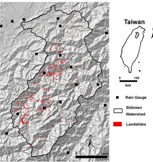
The 760 km2study area is located in the Shihmen Reservoir watershed in northern

Taiwan (Figure 1). Elevations in the watershed range from 135 m in the northwest to

3529 m in the southeast, with generally rugged topography. Nearly 90% of the study

area is forested. The climate is influenced by typhoons in summer and the northeast

monsoon in winter. The mean annual temperature is 21oC, with a mean monthly

temperature of 27.5oC in July and 14.2oC in January. The annual precipitation

averages 2370 mm. Because of the aforementioned typhoons, large rainfall events

Figure 1. Study area and landslides triggered by Typhoon Aere.

2.2. Typhoon Aere

Taiwan is an island, about 380 km long and 140 km wide, separated by the Strait of

Formosa from southeastern China. The island is prone to an average of four to five

typhoons originating from the Pacific each year. These intense storms bring torrential

rains that trigger landslides in the Central Mountain Range (CMR), which occupies

almost two thirds of the island in a north-south orientation. From August 23 to 25,

before turning southwestward. The typhoon affected Taiwan, especially the northern

half, for three days. During its peak intensity on August 24, Typhoon Aere had a

200-km storm radius and a low pressure reading of 955 mb, packing winds of 140 km

hr-1and gusts to 175 km hr-1. Thirty-four people were killed as a result of the storm,

including 15 died as a landslide buried a remote mountain village in the north. The

passage of Typhoon Aere brought 1604 mm of rainfall to the study area, with a

maximum 24-hr intensity of 51.7 mm hr-1(CWB 2004). The silt accumulation from

the upland landslides and stream scouring forced to stop the outlet of drinking water

from the Shihmen Reservoir and jammed the water supply pipes for days (Chen et al.

2006). Based on the damage to properties and human lives, Typhoon Aere was the

worst typhoon that struck northern Taiwan in recent years.

2.3. Landslide Data

Landslides triggered by Typhoon Aere were interpreted and delineated by comparing

ortho-rectified aerial photographs taken before and after the typhoon. These colour

orthophotographs were compiled by theAerialSurvey OfficeofTaiwan’sForestry

Bureau from the stereo pairs of 1:5000 aerial photographs. They have a pixel size of

0.35 m and an estimated horizontal accuracy of 0.5 m. For model validation, this

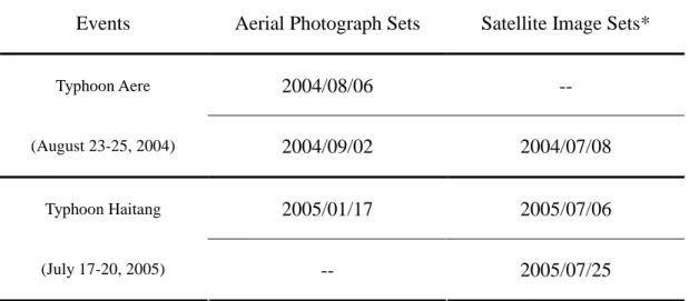
study interpreted and delineated landslides triggered by Typhoon Haitang (July 17 to

dates of flights of aerial photographs and satellite images.

Table 1. Image data sources

Events Aerial Photograph Sets Satellite Image Sets*

2004/08/06 --Typhoon Aere (August 23-25, 2004) 2004/09/02 2004/07/08 2005/01/17 2005/07/06 Typhoon Haitang (July 17-20, 2005) -- 2005/07/25

-- No Images; *2-m FORMOSAT-2 panchromatic images.

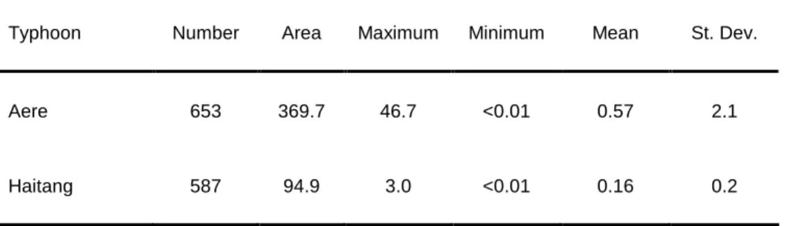
Typhoon Aere triggered 703 landslides of which 50 were enlarged or reactivated

old landslides. Typhoon Haitang triggered 1042 landslides of which 455 occurred on

existing landslides. Most observed slope failures were shallow landslides on soil

mantled slopes with depths less than 2 m. To develop our model, we only considered

new landslides triggered by typhoons: 653 by Aere, covering 4.87% of the study area;

and 587 by Haitang, covering 2.18% of the study area. Figure 1 shows the spatial

distribution of landslides triggered by Typhoon Aere, and Table 2 summarizes the

Table 2. Descriptive statistics of landslide areas (ha) triggered by typhoons

Typhoon Number Area Maximum Minimum Mean St. Dev.

Aere 653 369.7 46.7 <0.01 0.57 2.1

Haitang 587 94.9 3.0 <0.01 0.16 0.2

2.4. Rainfall Radar Data

Taiwan has over 400 rain gauge stations of which most are located in the lowland

areas on the west side of the mountain range. To better understand the spatial

distribution of precipitation in mountainous areas, the CWB has collaborated with the

U.S. National Oceanic and Atmospheric Agency’s National Severe Storms Laboratory

to deploy the QPESUMS system (quantitative precipitation estimation and

segregation using multiple sensors) (Vieux et al. 2003). The system uses four Doppler

weather radar (WSR-88D) sites to cover the island and the adjacent ocean. It records

base reflectivity with a spatial resolution of 0.0125° (~ 1.25 km) in both longitude and

latitude and a temporal resolution of 10 minutes.

The CWB provided radar base reflectivity data for August 23 to 25, 2004,

corresponding to the event of Typhoon Aere, for the study area. We also secured

ground rainfall measurements for the same time period from 19 automatic rain gauges

reflectivity data and rainfall measurements associated with Typhoon Haitang for

model validation.

3. Analysis

3.1. Rainfall Estimation

Developed by the CWB, the method for estimating ground-level area rainfall from

radar measurements involves two basic steps. First, radar reflectivity Z, measured in

decibels (db), is converted into rainfall rate R, measured in mm hr-1, by the following

Z-R power relationship (Marshall et al. 1947; Wilson 1970):

Z = 32.5R1.65 (1)

The parameter values of 32.5 and 1.65 proposed by Xin et al. (1997) are reported to

be more accurate than other values for fast moving convective storms.

Rainfall estimates can be improved when rain gauge observations are used to

calibrate radar data (Brandes 1975). The calibration method developed by the CWB

uses the inverse distance weighted method (IDW) to first create a grid representing

the deviations between R and hourly rainfall measurements. IDW is a spatial

interpolation method. The weight for IDW is defined by:





i,Withe weight at rain gauge i, and d_ithe distance between cell 0 and rain gauge i. To

complete the calibration, the deviation grid is added to the R grid to calculate the final

calibrated rainfall grid.

For this study, we summed the 10-minute radar reflectivity data by hour and

divided the sum by six for the hourly average. Then we followed equations (1) and (2)

to convert the hourly average reflectivity data into hourly rainfall data. This

conversion was performed for typhoons Aere and Haitang. The projection of the

hourly rainfall grid from geographic to plane coordinates resulted in a 36 by 55 grid

with a spatial resolution of 1 km.

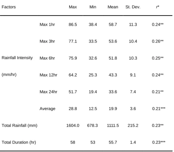
Using the hourly rainfall data, we derived various measures of rainfall intensity,

total, and duration associated with Typhoon Aere. Figures 2a, 2b, and 2c display the

maximum 3-hr rainfall intensity, total rainfall, and total duration, respectively. The

spatial distributions of maximum 3-hr rainfall intensity and total rainfall show similar

pattern. Both have the highest values in the southwestern and western parts of the

watershed, near the ridge that faced the dominant southwesterly and westerly winds

during the passage of Typhoon Aere. Table 3 shows the descriptive statistics of these

various rainfall factors as well as the correlation coefficients (r) between landslide

density (number of landslides km-2) and each factor. Maximum 3-hr intensity and

differences are small.

rainfall duration) and rain gauges (d).

Table 3. Rainfall factors and statistics

Factors Max Min Mean St. Dev. r*

Max 1hr 86.5 38.4 58.7 11.3 0.24** Max 3hr 77.1 33.5 53.6 10.4 0.26** Max 6hr 75.9 32.6 51.8 10.3 0.25** Max 12hr 64.2 25.3 43.3 9.1 0.24** Max 24hr 51.7 19.4 33.6 7.4 0.21** Rainfall Intensity (mm/hr) Average 28.8 12.5 19.9 3.6 0.21*** Total Rainfall (mm) 1604.0 678.3 1111.5 215.2 0.23** Total Duration (hr) 58 53 55.7 1.4 0.23***

*Correlation coefficient between rainfall factor and landslide density

** Significant at 1% level

*** Significant at 5% level

3.2 Logistic Regression

Logistic regression is useful when the dependent variable is categorical (e.g., presence

or absence) and the explanatory variables are categorical, numeric, or both (Menard

2002). The logit model from a logistic regression has the following form:

where the logit of y is the dependent variable, xiis the explanatory variable i, a is a

constant, biis the regression coefficient i, and e is the error term. The logit of y is the

natural logarithm of the odds: logit (y) = ln ) 1 ( p p  (4)

where p is the probability of the occurrence of y and p/(1 - p) is the odds. To convert

logit (y) back to the probability p, equation (4) can be rewritten as:

...) exp( 1 ...) exp( 3 3 2 2 1 1 3 3 2 2 1 1           x b x b x b a x b x b x b a p (5)

A logit model can be evaluated by the receiver operating characteristic (ROC).

The ROC measures the fitness of a model on the basis of true positive (proportion of

incidences correctly reported as positive) and false positive (proportion of incidences

erroneously reported as positive) (Pontius and Batchu, 2003). Typically, a probability

value of 0.5 is used to determine whether the model has made a correct prediction (>

0.5) or not (< 0.5). Additionally, Cox and Snell R2and Nagelkerke R2measure how

well the explanatory variables can predict and explain the dependent variable. Cox

and Snell R2cannot achieve a maximum of 1, whereas Nagelkerke R2stretches the R2

value to range from 0 to 1.

For this study, the dependent variable (y) represented landslide (1) or stable area

cell (0) and the explanatory variables were maximum 3-hr rainfall intensity (x1) and

in previous studies can be generally grouped into two categories. The first category

uses rainfall intensity and duration (Caine 1980; Cannon and Ellen 1985; Larsen and

Simon 1993; Finlay et al. 1997; Aleotti 2004; Godt et al. 2006), and the second uses

total or cumulative rainfall (Au 1993; Dai and Lee 2003; Guzzetti et al. 2004; Ibsen

and Casagli 2004). This study followed the first category of studies but chose

maximum 3-hr rainfall intensity instead of average intensity because maximum 3-hr

rainfall intensity had a slightly higher r value with landslide density.

4. Results

4.1. Logit Model

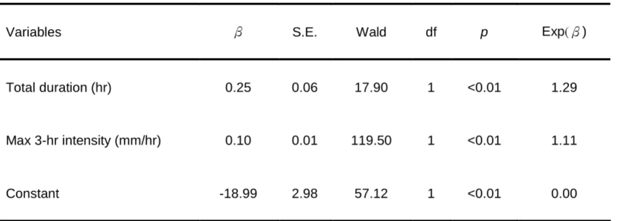
The logit model is significant at the 0.01 level, with ROC = 0.76, Cox & Snell R2=

0.27, and Nagelkerke R2= 0.36. Both explanatory variables are significant at the 1%

level, with total duration being slightly more important than maximum 3-hr intensity

in explaining landslide occurrence (Table 4).

Table 4. Logistic regression resultsa

Variables β S.E. Wald df p Exp(β)

Total duration (hr) 0.25 0.06 17.90 1 <0.01 1.29

Max 3-hr intensity (mm/hr) 0.10 0.01 119.50 1 <0.01 1.11

Constant -18.99 2.98 57.12 1 <0.01 0.00

a

the standard error (S.E.) given. The Wald statistic is the ratio of theβto S.E. of the

regression coefficient squared. df is the degree of freedom. The significance of each

explanatory is given by the p value. Exp(β) is the predicted change in odds for a unit

increase in the explanatory variable.

4.2. Critical Rainfall Conditions

To use rainfall data for predicting landslides, critical rainfall intensity and total

duration can be derived from the logit model. Substituting logit (y) by equation (4)

and ignoring the error term, equation (3) becomes:

2 2 1 1 ) 1 ln( a b x b x p p     (6)

Equation (6) can be rewritten as:       _{ }   ) ( ) 1 ln( 1 2 2 1 1 b x a p p b x (7)

By specifying the p value (e.g., 0.5) and an x2value in equation (7), we can compute a

corresponding x1value. By going through the computation twice, we can get two pairs

of x1and x2values to plot a straight line representing the specified p value (e.g., 0.5).

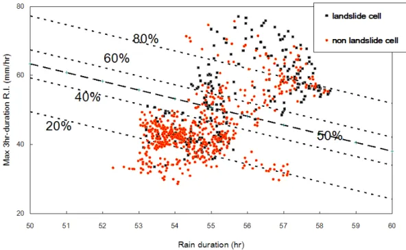
Figure 3 shows such lines representing the probabilities of landslide occurrence at 0.2,

0.4, 0.5, 0.6, and 0.8. Equation (7) is hereafter referred to as the probability model.

Figure 3 also shows dots for landslide and stable-area cells. The location of a dot or

cell corresponds to its maximum 3-hr rainfall intensity and total duration values, and

landslides triggered by Typhoon Aere against calculated probabilities from equation

(7). As to be expected, most landslides fall within areas of high probabilities.

Figure 3. Critical rainfall conditions for triggering landslides. The lines show different

Figure 4. Probability maps of landslide occurrence derived from the model and

landslides triggered by Typhoon Aere (a) and Typhoon Haitang (b).

4.3 Model Validation

Landslides triggered by Typhoon Haitang were used for validating the probability

model derived from the landslide and rainfall data associated with Typhoon Aere.

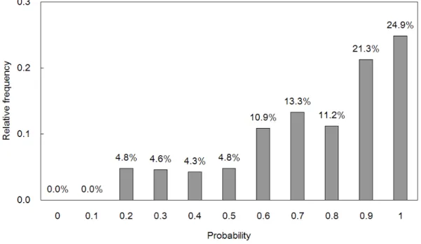
Using 0.5 as the threshold, the model correctly predicted 81.6% of landslides

triggered by Typhoon Haitang. In other words, 81.6% of landslides fall within areas

with probabilities greater than 0.5 as predicted by the model (Figure 5). This is

visually confirmed in Figure 4b, which plots landslides triggered by Typhoon Haitang

against calculated probabilities from equation (7).

Figure 5. A comparison of relative frequencies of landslides triggered by Typhoon

rainfall data associated with Typhoon Aere.

5. Discussion

5.1. The Probability Model vs. Minimum Rainfall Threshold

The probability model that this study has developed differs from minimum rainfall

thresholds of previous studies in two fundamental aspects. First, the probability model

is a spatially explicit model, which is based on logistic regression that statistically

separate landslides from stable areas by maximum 3-hr rainfall intensity and rainfall

duration. In contrast, a minimum rainfall threshold represents the lower bound of a

log-log plot of rainfall data that have resulted in landslides without considering the

locations of landslides and stable areas. Second, the probability model computes a

probability for a given combination of rainfall values and offers a measure of the

likelihood of landslide occurrence. In comparison, a minimum rainfall threshold

simply suggests that, if a rainfall event exceeds the threshold, it will likely trigger

landslides. No measure of confidence is provided with such prediction. Given these

two differences, we feel that the probability model is better suited for a landslide

monitoring or warning system than the minimum rainfall threshold.

5.2. Radar Data for Landslide Studies

The high spatial and temporal resolutions of the NEXRAD reflectivity imagery are

based. But the Z-R relationship for converting radar reflectivity data to rainfall rate

can be complicated by ground clutter, beam blockage, close clustering of cells, and

differences in precipitation echoes between water droplets and ice particles and

between different-sized water droplets (Howard et al. 1997; Steiner and Smith 2002;

Wilson 2005).

This study adopted a method developed by Taiwan’s CWB for estimating rainfall

from radar measurements. Because we used all 19 automatic gauge stations in and

around the study area for calibration, we could not perform an accuracy assessment of

radar-derived rainfall data. However, previous studies have shown the robustness of

the CWB method. Based on two typhoon events, Chang et al. (2006) reported that

calibrated rainfall estimates from QPESUMS reflectivity imagery deviated from

ground measures of 100 gauge stations in Taiwan by less than 1 mm for hourly

rainfall, 12 to 34 mm for daily rainfall, and 29 to 79 mm for total rainfall. Chen et al.

(2007) found that calibrated rainfall data by QPESUMS estimation agreed well with

those from four ground-based stations in central Taiwan, with the correlation

coefficients all above 0.9 between the two. Both studies therefore support the

QPESUMS system and the CWB method for rainfall estimation.

Rainfall data derived from QPESUMS imagery have a spatial resolution of 1.25

of ground-based rain gauges, it still cannot match that of landslides delineated and

mapping on aerial photographs or high-resolution satellite images. On the other hand,

landslide data cannot match the temporal resolution (10 minutes) of QPESUMS

imagery. In fact, the timing of landslides is usually gathered from interviews of local

residents and its accuracy can only be described as reasonably accurate (e.g., Guzzetti

et al. 2004). The incompatibility of scales/resolutions is common in landslide studies

(e.g., 1:5000-scale soil map vs. 1:100,000-scale geology map), but it can create

problems in interpreting and applying results. How to match landslide and rainfall

data in both spatial and temporal resolutions is certainly an important topic for future

investigation.

5.3 Applications of the Model

The probability model that this study has developed is simple to use: given maximum

3-hr rainfall intensity and total rainfall duration, the model computes probabilities for

landslide occurrence on a cell basis. It can be part of a real-time landslide monitoring

system in which the two rainfall variables calculated from the QPESUMS system are

entered to compute the probability of landslide occurrence at a regular interval (e.g.,

every six hours) during a typhoon event. The probability map thus derived will show

which areas are likely to have landslide occurrence, and the difference in probability

The model can also be used as an aid for landslide delineation and mapping

following a typhoon event. A mask based on the model or a model with additional

variables can highlight areas that are more likely to have landslides, thus facilitating

such tasks as coordinating mitigation efforts. For example, if we add elevation, slope,

and lithology as explanatory variables to the logit model in this study, the model has

ROC = 0.78, Cox & Snell R2= 0.32, and Nagelkerke R2= 0.42. This model can

therefore better assist in locating areas that are more prone to landslides than the

initial logit model with only two rainfall variables.

But to use the probability model for a landslide warning system will require a

robust typhoon precipitation model at a high spatial resolution. Because Taiwan is

extremely vulnerable to the damages from typhoons, numerical models for simulating

typhoons have been a top research priority (Wu and Kuo 1999). The fifth-generation

Pennsylvania State University-National Centre for Atmospheric Research Mesoscale

Model (MM5) has been used in several recent studies to simulate the rainfall

distribution associated with a typhoon (Wu et al. 2002; Witcraft et al. 2005; Yang and

Ching 2005). A typhoon rainfall climatology-persistence (R-CLIPER) has also been

used for rainfall estimation in the 2004 and 2005 typhoon seasons (Cheung et al.

2006). Although these studies all reported good simulation or prediction results, they

spatial scale issue must be resolved before the integration of a typhoon model and this

study’s landslide probability model can be realised for a watershed-level warning

system.

6. Conclusion

This study compiled Doppler weather radar reflectivity data during Typhoon Aere

(August 2004), estimated rainfall from radar data, and used maximum 3-hr rainfall

intensity and rainfall duration as the explanatory variables in logistic regression for a

landslide prediction model. The logit model had a ROC of 76%. Results of model

validation showed an accuracy rate of 82% in predicting landslides triggered by

Typhoon Haitang (July 2005). This cell-based model can be part of a landslide

warning system by incorporating predicted rainfall data from a typhoon precipitation

model. It can also be part of a real-time landslide monitoring system by being able to

compute probabilities of landslide occurrence at a regular interval during a typhoon

event. Finally, the model can be used as an analysis mask for landslide delineation and

mapping following a typhoon event. Compared to minimum rainfall thresholds of

previous studies, this probability model has the distinct advantage of providing a

measure of confidence in predicting landslides and landslide locations associated with

a typhoon event.

approach to incorporate rainfall into landslide modelling and prediction. Further

improvement of the model requires a better integration of landslide data, radar

reflectivity data, and estimated typhoon precipitation data in both spatial and temporal

References

Aleotti P. 2004. A warning system for rainfall-induced shallow failures. Engineering

Geology 73: 247-265.

Au SWC. 1993. Rainfall and slope failure in Hong Kong. Engineering Geology 36:

141-147.

Ayalew L, Yamagishi, H. 2005. The application of GIS-based logistic regression for

landslide susceptibility mapping in the Kakuda-Yahiko Mountains, Central Japan.

Geomorphology 65: 15-31.

Barm RL, Coe JA, Godt JW, Harp, EL, Reid ME, Savage WZ, Schulz WH, Brien DL,

Chleborad AF, McKenna JP, Michael JA. 2005. Regional landslide-hazard assessment

for Seattle, Washington, USA. Landslides 2: 266-279.

Brandes EA. 1975. Optimizing rainfall estimates with the aid of radar. Journal of

Applied Meteorology 14: 1339-1345.

Caine N. 1980. The rainfall intensity-duration control of shallow landslides and debris

flows. Geografiska Annaler 62A: 23-27.

Campbell RH. 1975. Soil Slips, Debris Flows, and Rainstorms in the Santa Monica

Mountains and Vicinity, Southern California. USGS Professional Paper 851. US

Geological Survey: Reston, VA.

San Francisco Bay region, California. California Geology 38: 267-272.

Cannon SH, Gartner JE, Wilson RC, Bowers JC, Laber JL. 2007. Storm rainfall

conditions for floods and debris flows from recently burned areas in southwestern

Colourado and southern California. Geomorphology, in press. DOI:

10.1016/j.geomorph.2007.03.019.

Cardinali M, Galli M, Guzzetti F, Ardizzone F, Reichenbach P, Bartoccini P. 2006.

Rainfall induced landslides in December 2004 in Southwestern Umbria, Central Italy.

Natural Hazards and Earth System Sciences 6: 237-260.

Casadei M, Dietrich WE, Miller NL. 2003. Testing a model for predicting the timing

and location of shallow landslide initiation in soil-mantled landscapes. Earth Surface

Processes and Landforms 28: 925-950.

Chang C, Sun C, Lay J. 2006. Integration of radar detection and real time rainfall data

for estimation during typhoon period. Environment and Worlds 13: 1-22. (in Chinese)

Chen C, Chen T, Yu F, Yu W, Tseng C. 2005. Rainfall duration and debris-flow

initiated studies for real-time monitoring. Environmental Geology 47: 715-724.

Chen C, Lee W, Yu F. 2006. Debris flow hazards and emergency response in Taiwan.

In Monitoring, Simulation, Prevention and Remediation of Dense and Debris Flows,

Lorenzini G., Brebbia CA, Emmanouloudis DE. (eds). WIT Press: Southampton,

Chen C, Lin L, Yu F, Lee C, Tseng C, Wang A, Cheung K. 2007. Improving debris

flow monitoring in Taiwan by using high-resolution rainfall products from QPESUMS.

Natural Hazards 40: 447-461.

Cheung KKW, Huang L, Lee C. 2006. A tropical cyclone rainfall

climatology-persistence model for the Taiwan area. Proceedings: 27thSymposium on

Hurricane and Tropical Meteorology, April 24-28, Monterey, CA.

Crozier MJ. 1999. Prediction of rainfall-triggered landslides: A test of the antecedent

water status model. Earth Surface Processes and Landforms 24: 825-833.

CWB (Central Weather Bureau). 2004.

http://photino.cwb.gov.tw/tyweb/tyfnweb/htm/2004aere.htm(accessed April 22,

2006).

Dai FC, Lee CF. 2003. A spatiotemporal probabilistic modelling of storm-induced

shallow landsliding using aerial photographs and logistic regression. Earth Surface

Processes and Landform 28: 527-545.

Finlay PJ, Fell R, Maguire PK. 1997. The relationship between the probability of

landslide occurrence and rainfall. Canadian Geotechnical Journal 34: 811-824.

Floris M, Bozzano F. 2007. Evaluation of landslide reactivation: a modified rainfall

threshold model based on historical records of rainfall and landslides. Geomorphology,

Glade T, Crozier MJ, Smith P. 2000. Applying probability determination to refine

landslide-triggering rainfall thresholds using an empirical “Antecedent Daily Rainfall

Model”. Pure and Applied Geophysics 157: 1059-1079.

Godt JW, Baum RL, Chleborad AF. 2006. Rainfall characteristics for shallow

landsliding in Seattle, Washington, USA. Earth Surface Processes and Landforms 31:

97-110.

Guzzetti F, Cardinali M, Reichenbach P, Cipolla F, Sebastiani C, Galli M, Salvati P.

2004. Landslides triggered by the 23 November 2000 rainfall event in the Imperia

Province, Western Liguria, Italy. Engineering Geology 73: 229-245.

Guzzetti F, Peruccacci S, Rossi M, Start CP. 2007. Rainfall thresholds for the

initiation of landslides. Meteorology and Atmospheric Physics, in press. DOI:

10.1007/s00703-007-0262-7.

Howard KW, Gourley JJ, Maddox RA. 1997. Uncertainties in WSR-88D

measurements and their impacts on monitoring life cycles. Weather and Forecasting

12: 166-174.

Ibsen M-L, Casagli N. 2004. Rainfall patterns and related landslide incidence in the

Porretta-Vergato region, Italy. Landslides 1: 143-150.

Iverson RM. 2000. Landslide triggering by rain infiltration. Water Resources Research

Marshall JS, Langille RC, Palmer WM. 1947. Measurement of rainfall by radar.

Journal of Meteorology 4: 186-191.

Meisina C, Scarabelli S.2007. A comparative analysis of terrain stability models for

predicting shallow landslides in colluvial soils. Geomorphology 87: 207-223.

Menard S. 2002. Applied Logistic Regression Analysis, 2d ed. Thousand Oaks, CA:

Sage.

Montgomery DR, Dietrich WE. 1994. A physically based model for topographic

control on shallow landsliding. Water Resources Research 30: 1153-1171.

Morrissey MM, Wieczorek GF, Morgan BA. 2004. Transient hazard model using

radar data for predicting debris flows in Madison County, Virginia. Environmental &

Engineering Geoscience 10: 285-296.

Ohlmacher GC, Davis JC. 2003. Using multiple logistic regression and GIS

technology to predict landslide hazard in northeast Kansas, USA. Engineering

Geology 69: 331-343.

Pack RT, Tarboten DG, Goodwin CN. 1999. GIS-based landslide susceptibility

mapping with SINMAP, Proceedings: 34th Symposium on Engineering Geology and

Geotechnical Engineering, April 28-30, Logan, Utah; 219-231.

Pontius RG, Jr., Batchu K. 2003. Using the relative operating characteristic to quantify

467-484.

Steiner M, Smith JA. 2002. Use of three-dimensional reflectivity structure for

automated detection and removal of nonprecipitating echoes in radar data. Journal of

Atmospheric and Oceanic Technology 19: 673-686.

Vieux BE, Vieux JE. 2003. Operational deployment of a physics-based distributed

rainfall-runoff model for flood forecasting in Taiwan. Paper presented at the

International Symposium on Information from Weather Radar and Distributed

Hydrological Modelling, July 7-8, 2003, Sapporo, Japan.

Wieczorek GF, Glade T. 2005. Climatic factors influencing occurrence of debris flows.

In Debris Flows Hazards and Related Phenomena, Jakob M, Hungr O. (eds). Springer:

Berlin; 325-362.

Wilson JW. 1970. Integration of radar and raingage data for improved rainfall

measurement. Journal of Applied Meteorology 9: 489-497.

Wilson RC. 2005. The rise and fall of a debris-flow warning system for the San

Francisco Bay region, California. In Landslide Hazard and Risk, Glade T, Anderson

M, Crozier MJ (eds). Wiley: Chichester, England; 493-516.

Witcraft N, Lin Y, Kuo Y. 2005. Dynamics of orographic rain associated with the

passage of a tropical cyclone over a mesoscale mountain. Terrestrial, Atmospheric

Wu C, Kuo Y. 1999. Typhoons affecting Taiwan: current understanding and future

challenges. Bulletin of the American Meteorological Society 80: 67-80.

Wu C, Yen T, Kuo Y, Wang W. 2002. Rainfall simulation associated with Typhoon

Herb (1996) near Taiwan, Part I: The topographic effect. Weather and Forecasting 17:

1001-1015.

Wu W, Sidle RC. 1995. A distributed slope stability model for steep forested basins.

Water Resources Research 31: 2098-2110.

Xin L, Reuter G, Larochelle B. 1997. Reflectivity-rain rate relationships for

convective rainshowers in Edmonton. Atmosphere-Ocean 35: 513-521.

Yang M, Ching L. 2005. A modelling study of typhoon Toraji (2001): physical

parameterization sensitivity and topographic effect. Terrestrial, Atmospheric and

Tom Veldkamp and Gerald Schoorl. Profs. Veldkamp and Schoorl are developers of

the LAPSUS (LandscApe ProcesS modelling at mUlti-dimensions and scaleS), a

multi-module dynamic landscape evolution model. Since the trip, we have been

working on a joint research project involving graduate students at National Taiwan

University and Wageningen University.

In September 2007 I was invited by KITAC Corp in Niigata, Japan to give a keynote

speech on my research work on rainfall-triggered landslides. Following the trip, I

have been working with Dr. Cheibany of KITAC Corp to test the critical rainfall

model that we have developed at National Taiwan University using precipitation and