在各類社會網絡模型下區域差異對於疾病與觀念流行傳播問題模擬之影響

全文

(1)國立交通大學資訊科學系碩士論文. 在各類社會網絡模型下區域差異對於疾病與觀念流行傳播問題模擬之影響. Influence of Local Information on Epidemic Simulation under Complex Networks. 研究生：鐘健銘指導教授：孫春在. 教授. 中華民國九十四年六月 i.

(2) 在各類社會網絡模型下區域差異對於疾病與觀念流行傳播問題模擬之影響 Influence of Local Information on Epidemic Simulation under Complex Networks 研究生：鐘健銘. Student：Chien-Ming Chung. 指導教授：孫春在. Advisor：Chuen-Tasi Sun. 國立交通大學資訊科學系碩士論文 A Thesis Submitted to Institute of Computer and Information Science College of Electrical Engineering and Computer Science National Chiao Tung University in partial Fulfillment of the Requirements for the Degree of Master in Computer and Information Science June 2005 Hsinchu, Taiwan, Republic of China. 中華民國九十四年六月 ii.

(3) 在各類社會網絡模型下區域差異對於疾病與觀念流行傳播問題模擬之影響學生：鐘健銘. 指導教授：孫春在. 教授. 國立交通大學資訊科學研究所摘要除了以複雜網路模擬人際互動關係外，區域差異的設計也是為了使社會傳播的模擬環境能夠更貼近真實社會。然而在先前的研究發現不同的區域差異對小世界網路所造成的影響力也不同，例如虛弱個體所占人口比例多寡會影響傳播強度而虛弱個體在社會上的分布範圍則不會。另外早期的研究由於不考慮人際關係因此類似以隨機網路為實驗平台，相較於使用小世界網路探討疾病動態有何不同之處。因此本論文的重點在於分析不同的網路結構以及區域差異對於傳播問題的影響力。並將結果整理成具有影響力的網路結構因素和傳播強度資訊以及不具影響力的細節資訊。. 關鍵字：複雜網路、區域資訊、社會模擬、傳播問題、小世界網路. iii.

(4) Influence of Local Information on Epidemic Simulation under Complex Networks Student: Chien-Ming Chung. Advisor: Dr. Chuen-Tsai Sun. Institute of Computer and Information Science National Chiao Tung University. ABSTRACT Besides using complex networks in epidemic simulation for unfolding the relationships between human beings, local information mechanism was designed to reveal the differences among people and others to approximate reality. However, previous studies indicate that some local diversity would not affect the simulation result. The population of weak individuals, for example, would cause the difference of simulation, but the distribution of weak individuals would not. Furthermore, we are also interested in the differences between the simulation under the small-world networks and the previous research without considering the relationship as simulation in the random networks. In this paper, we focused on the analysis of various network structures and local information, and conclude some reasons that might influence the epidemic simulations. Keywords: Complex network, local information, social simulation, epidemic simulation, small world model. i.

(5) 誌謝將要結束碩士班的兩年生活，首先感謝我的指導教授孫春在老師，是您的教誨使得我對問題的觀察角度有了新的認識，也對研究有了更深的體會。其次感謝實驗室的學長姐們，無論在課程上的修業或是研究內容上，你們都給了我莫大的幫助。尤其感謝崇源學長多次的與我辯論舌戰以決定某些內容的去留，可以說沒有你的幫忙就沒有這本論文；另外是吉隆學長，你在實驗室督促我們做研究寫論文的聲音是我永遠也忘不了的；謝謝你們。也感謝實驗室的同學其煜、承龍、仁鴻、端木、家胤、冠傑、東鴻、敬華、喬文、Camil，在這兩年來無數次的互相討論幫忙，讓我們得以順利度過每一次的考驗。最後是我的家人們，謝謝你們在我背後默默的支持著，讓我能順利的完成這個碩士學位，爸、媽、姐、弟、還有奕婷，感謝你們的陪伴，我永遠愛你們。. ii.

(6) Content ABSTRACT ............................................................................................................................................ I 1. INTRODUCTION.........................................................................................................................1. 2. BACKGROUND ...........................................................................................................................4 2.1. SMALL-WORLD PHENOMENA .................................................................................................4. 2.2. COMPLEX NETWORKS ............................................................................................................6. 2.3. SIR MODEL WITH COMPLEX NETWORKS ................................................................................9. 3. NETWORK MODELS IN THE EXPERIMENTS .................................................................. 11. 4. CONTAGION MODELS ...........................................................................................................13. 5. LOCAL INFORMATION MECHANISM................................................................................16. 6. THE EXPERIMENTS................................................................................................................17. 7. 6.1. NETWORK STRUCTURE ANALYSIS ........................................................................................17. 6.2. WEAK INDIVIDUAL PROPORTIONS ........................................................................................20. 6.3. DISTRIBUTION PATTERNS OF WEAK INDIVIDUALS ................................................................22. 6.4. FAMILIAR PAIRS AND ONE-WAY CHANNELS PROPORTIONS ....................................................24. 6.5. DISTRIBUTION PATTERNS OF FAMILIAR PAIRS .......................................................................28. CONCLUSION ...........................................................................................................................30. APPENDIX A複雜網路........................................................................................................................31 APPENDIX B 傳播問題建模..............................................................................................................36 REFERENCE .......................................................................................................................................39. iii.

(7) List of Figures FIG. 2-1 REGULAR NETWORK ....................................................................................................................7 FIG. 2-2 THREE TYPES OF NETWORKS .........................................................................................................8 FIG. 3 INPUT OF THE ASSUMPTION ............................................................................................................ 11 FIG. 4-1 SIR MODEL.................................................................................................................................14 FIG. 6-1 RESULTS OF VERTEX DEGREE DISTRIBUTION...............................................................................18 FIG. 6-2 RESULTS OF NETWORK STRUCTURES ANALYSIS ..........................................................................19 FIG. 6-3 WEAK INDIVIDUAL PROPORTION IN WATTS’ NETWORKS .............................................................20 FIG. 6-4 WEAK INDIVIDUAL PROPORTION IN RANDOM NETWORKS ...........................................................21 FIG. 6-5 WEAK INDIVIDUAL PROPORTION IN SCALE-FREE NETWORKS ......................................................22 FIG. 6-6 THE RADIUS REPRESENTATION ....................................................................................................23 FIG. 6-7 DISTRIBUTION PATTERNS OF WEAK INDIVIDUAL IN SMALL-WORLD NETWORKS ..........................23 FIG. 6-8 SMALL-WORLD NETWORKS ........................................................................................................25 FIG. 6-9 RANDOM NETWORKS ..................................................................................................................25 FIG. 6-10 SCALE-FREE NETWORKS ...........................................................................................................26 FIG. 6-11 SMALL-WORLD NETWORKS ......................................................................................................26 FIG. 6-12 RANDOM NETWORKS ................................................................................................................27 FIG. 6-13 SCALE-FREE NETWORKS ...........................................................................................................27 FIG. A-1 規則網路與小世界網路..........................................................................................................32 FIG. A-2 隨機網路 .................................................................................................................................33 FIG. A-3 無尺度網路 .............................................................................................................................34 FIG. B-2 實驗流程圖 .............................................................................................................................38. iv.

(8) 1 Introduction In the beginning, the epidemic simulation was performed by dynamic systems [1]. With the introduction of Monde Carlo model, researchers started to have the concept of individual in the simulation [2]. Without considering the interactions between human beings, Monde Carlo model just like SIR model, which was still another simple model of simulating a disease among several compartmental groups, can not show the real properties of society with epidemic outbreaks. Because the interactions among several compartmental groups could be under consideration in simulating circumstances, researchers started to combine SIR model with complex networks after that were proposed successively. Complex networks are often used to described a virtual social network, where exist groups of related individuals that are interacting with each other [3]. Small world networks, scale-free networks, random networks, and regular networks are in the field of complex networks.. Recently, researchers used the complex networks to investigate in disease spread and cultural dissemination by use of SIR model. They could observe the propagation of diseases or rumors among society, even suggest some control measures for disease, such as the contagion of SARS and AIDS even for the spread of rumors [4-6]. However, with the differences among all types of the contagion problems, we have to use suitable network models to simulate the relationship networks. Take AIDS for example. Its routes of infection is far from the influenza’s, it should be noticed that we cannot use the same model to analyze them. Generally, the small world model is used to simulate the epidemic propagation and rumors spreading, while scale-free network model for the study of AIDS contagions. Therefore, the fundamental. 1.

(9) meanings of different structure of social network models are extremely different.. Besides, there also exist other parameters such as attribute information, weight information, and so on. Regarding to aforementioned local information, researchers should cautiously collect pieces of information from all aspects to construct a proper simulating environment Take previous case of simulating epidemic outbreak for example, first we have to know how many cases we input initially. Further more, we have to know the percentage of the weak individuals among the whole population, and how they distribute in the society. Of course, the divergences among the local information will become a hard job in information gathering and content analyzing for the settings in the experiments.. Nevertheless, such variances as the different individuals or the weight information will not lead to the same results in different models. Like the experiments in this thesis(which we will mention later) , we discover that the distribution of the weak individuals does not reveal an obvious susceptibility in any kind of models, while the percentage of the those among the whole population show an remarkable effects to the results.. In order to realize what variances of local information result in some kind of effects under the circumstance of any specific models, we find out that some researchers have studied the effectiveness of the different individuals in small world networks [7]. Therefore, the main point of the thesis will aim to the analysis of different network structures and the effectiveness resulted from the variance of local information in contagion problems. After getting the researches about the local information in contagion problems together, we will talk over the effectiveness caused 2.

(10) by the following five local variances. First, we will discuss how different ways for constructing networks affect the vertex degree of information. Second, while constructing networks, various shortcut numbers would be significant. Third, the variances caused by the amount of heterogeneous individuals in the whole population and distribution will be discussed. Finally, the weights and the directions of the connections of individuals are concerned. We believe that the experimental results will help to further social contagion issues studies.. 3.

(11) 2 Background 2.1 Small-World Phenomena More and more social issues are studied since Watts and Strogatz proposed small-world network model [8]. For this reason, small-world phenomena [9] which influenced Watts and Strogatz extremely are discussed with variance of complex networks. Although many quantities and measures of complex networks have been proposed and investigated, but what researchers most concerned about were average path length, clustering coefficient, and vertex degree. We will take a brief introduction of these networks’ concepts.. Average Path Length： Average path length mainly describes that two nodes communicate with each other in a network probably pass through how many paths. Suppose that d ij represents the minimum paths from node i to node j , and Dij represents the maximum paths from node i to node j . Then average path length between these two nodes would be. d ij + Dij 2. , and average path length of a network model is. averaged all pair of nodes’ average path length. Generally speaking, average path length depends on the size of a network. Take six degree separation for example, two arbitrary people in real world can be link up with no more than six people. And for a small group, the average path length would be 1 because of every one have acquaintance with each other. Normally, for approximate to real world, researchers would set up experiment’s parameters by any reference material. Think about the six degree separation of real 4.

(12) world which contains six billion people, and the distance between two nodes increases logarithmically with expanding system size [10]. Say, a virtual society’s average path length should be 2.45 with ten thousand individuals. Therefore, there should be 17 shortcuts besides 4 neighbors. But in some social simulation experiments’ small-world model, they would set shortcuts less than this. We will analyze this unusual problem in this paper.. Clustering Coefficient： In real world, my friend’s friend would be my friend also. On the other hand, two of my friends probably may be friends with each other. It represents that most people are clustered together by “friends”. Clustering coefficient mainly says the probability of being friends mutually among a group. Clustering effect in regular network and small-world network is quite obvious by linking up with neighbors of all nodes at initial state. On the contrary, random network and scale-free network are not been setting any edges with neighbors, such that we can’t find out clustering effect. Suppose that clustering coefficient C i of individual i in the social network and this node links up with k i nodes. Obviously, there are no more than. ki ( ki − 1) 2. edges exist among them. Then clustering coefficient of node i is defined as. Ci ≡. Ei. k i (k i − 1) 2. . The E i represents exactly edge numbers exist among the group.. And the clustering coefficient of whole network is the average of C i over all i .. Vertex Degree： What is most important characteristic of a node in network may be the vertex degree. The more vertex degree of a node, the more related individuals it has. Either. 5.

(13) the spread of rumors or the infection of diseases, the probability of expanding is larger than other nodes which are in low branches. Usually, a person who is good at communication in a group and this man has a good relationship with the others, so that we will pass the message through him for efficiency. Vertex degree distribution is determined by construction network model. Scale-free network with power-law is extremely different from small-world network or random network with identity degree distribution. Even in small-world network models, different vertex degree settings can make virtual society closed to real world. Therefore, degree of vertices will be a significant index in different models.. 2.2. Complex Networks. According to average path length, clustering coefficient, and vertex degree distribution these three small-world phenomenon, complex networks can be categorized as below.. Regular Networks： As shown in figure 2-1, it’s a simple regular network. All individuals in a regular network just link up with neighbors. Since every node only has local edges, so we can determine a parameter of distance d , what represents it’s all relative within the distance.. However, all small-world phenomenon is decided by the value of d . It will be a complete graph while d is maximum, then there is lowest average path length, highest clustering coefficient, and highest vertex degree. What a circumstance may be. 6.

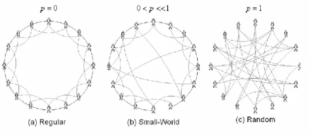
(14) horrible with contagion problem. Imagine that a traditional village, a bad guy is talked by some villagers. And 2 or 3 days later, everyone in the village knows about the bad guy. The powerful contagion is because of villagers know almost each other. But if. d equals to 1, it means all individuals just link up with neighbors. Then the highest average path length, lowest clustering coefficient and vertex degree will be occurred. Such environment has bad efficiency in contagion problems.. Fig. 2-1 Regular Network. Random Networks： In opposition to regular networks are random networks which proposed by Erdös and Rényi [11], generating a random network is adding links between pairs of randomly chosen nodes, or rewiring all edges in a regular network. If sufficient numbers of links are added, this kind of networks may exhibit small-world properties but with little or no clustering, what is an unusual situation in the real world.. Small-World Networks： It indicates that it is a high clustering and low separation society in the real world 7.

(15) in recent researches [12]. Using regular networks to construct a virtual society like the real world, we have to let the network model close to a complete graph without rationality. In order to make it sense, the small-world networks modified by Newman and Watts, which used adding shortcuts instead of rewiring [13], are used more often. A small-world network is generated by inserting long-range links which is called shortcuts into an n-dimension regular network [8]. Thus it can reserve the clustering property, and reduce the average path length to suitable to the real world. Using rewiring method to construct networks above, we can arrange the result as figure 2-2 by p, which is rewiring probabilities.. Fig. 2-2 three types of networks In this regular network (figure2-2a), every node just interacts with 4 neighbors. Without shortcuts, this model shows high clustering and separation, and all vertex degree is 4. Rewiring some links we can see a small-world network shown as figure 2-2b. In addition to all vertex degree are near 4, some individuals has shortcuts for interacting with long-range individuals. Besides, friends acquaint with each other makes it represents high clustering and low separation. The extreme random network model (figure 2-2c) is generated by rewiring all links, such that friends became unfamiliar with each other. So it is low separation but low clustering.. 8.

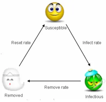
(16) That is homogenous vertex degree of the networks above. On the contrary of scale-free networks which investigated recently represent the power-law degree distribution. In the real world, sexual intercourse, internet hyperlink, and so on, belong to this type of model.. Scale-Free Networks： The power-law of vertex degree distribution is the most important property in scale-free networks [14-16]. It means most individuals have fewer links but fewer individuals have many links. Take the sexual intercourse for example, most of us are single mate, but some have many lovers. Such as internet hyperlink is also this situation. So it is suitable for venereal disease or internet virus studies by using scale-free networks. Generating a scale-free network begins with a small number of nodes which denoted as m0. [3]. Then recurring let a new node connects to m ≤ m0 preexisting. nodes picked from the group by probability p which determined by vertex degree of the node. New nodes are preferentially attached to existing nodes that have large numbers of connections.. 2.3 SIR model with Complex Networks Tracing the contagion problems to its source is SIR model proposed by Kermack and McKendrick [17]. The SIR model describes how individual changes when became ill, which are classified as three types. S (Susceptible) means the healthy body with low resistance. I (Infectious) means the ill individual and a source of infection. R (Removed/Recovery) shows that the individual is dead or recovered. Without illness, 9.

(17) recovered bodies can’t infect others, and the probability of being illness again becomes low.. In early studies of contagion, three type groups in SIR model interact with complete random, that equals to investigate contagion in random networks. Although this hypothesis is not meet the reality, but a simplistic model without detailed setting is convenient for researchers. They just have to consider the disease’s ability and the number of infector at initial. Adding to passed studies, a roughly simulation of contagion is then constructed.. However, during the process of contagion, there is a close relationship between the propagation of disease or rumors and different network topology of interpersonal relationship. Thinking about the interaction of humans, in addition to household and friends, we may communicate with a restaurant-owner. Random networks can’t represent whole situation. Besides, there is some difference in detail of contagions. Thus, different network models are needed for various epidemic problems [18-20].. Generally, the small world model is used to simulate the epidemic propagation and rumors spreading, and scale-free network model for the study of sexual diseases contagions, and computer virus spreading. Therefore, we would discuss contagion problem with these two networks mainly, and compare the results to random networks and regular networks which were not similar to real world.. 10.

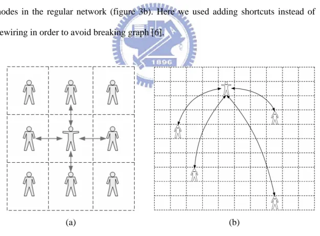
(18) 3 Network Models in the Experiments According to traditional cellular automata, we used a 100x100 2-D lattice to generate the complex networks as the platform in this paper, and investigated the transformation of these ten thousand individuals. In these virtual societies, all individuals would interact with others by edges only.. Each individual with 4 nearest neighbor links as the level one von Neumann Neighborhood in 2-D lattice was the regular network (figure3a). We thought such the circumstance as the family with five population was similar to reality. The small-world network was generated by adding several shortcuts between random nodes in the regular network (figure 3b). Here we used adding shortcuts instead of rewiring in order to avoid breaking graph [6].. (a). (b) Fig. 3 Input of the assumption. Furthermore, we used three ways to construct different small-world networks for our investigation of local information. We set a new weighted property d (v) of all 11.

(19) nodes, and let P(vi ) =. d (v i ) be the probability of node i which would be ∑ d (v ). v∈V ( G ). picked for adding shortcuts. The higher probability an individual had, the easier it was chosen to connect with others. The function of probability was classified into three ways below for closing reality, constant, normal, and uniform distribution. Firstly, constant distribution meant all individuals had equally probability. Secondly, we made the chosen probability of all nodes representing normal distribution. Finally, in uniform distribution, we divided all individuals into three parts with particular probability each.. The random network was generated by adding several shortcuts in 2-D lattice without nearest-neighbor links. In order to remain the property of random networks, we would not use the probability when adding nodes. We just picked several node-pairs complete randomly.. Lastly, for constructing the scale-free networks, we set the weighted property d (v) as small-world networks for all nodes. At the initial stage, all d (v) were set to. 1. Then we connected two nodes randomly, and increased the d (v) of these two nodes by 1, which made these nodes be picked easier later. Repeating the steps, we had the virtual society of scale-free networks.. 12.

(20) 4 Contagion Models Contagion problems are concerned about how infectious individuals affect accepters via certain infection channel. In epidemiology, infectious individuals are the patients. They make healthy people become infectious by direct contact or air spreading, the routes of infection. When talking about beliefs, missionaries play the role as the infectious ones, spread their beliefs in words or newspaper and magazines, making people inspired and have the belief too. Where words, newspaper and magazines are the routes of infection, and those who are called are the accepters. From the examples above, we can tell that contagion problems are composed of three individuals, infectious ones, routes of infection, and accepters.. In this article, we use all kind of social network models as the simulation platforms. Owing to the properties will distinct from one kind of contagion problem to another, we will discuss them through from random networks, small world networks, to scale-free networks. Besides, we use SIR model (figure 4-1) to simulate the propagation of ergodic individuals, expecting to show the process of how infectious individual take use of the connections in the networks as their channel.. 13.

(21) Fig. 4-1 SIR model. We can tell that when observing the phase transition of each individual, it is possible that a susceptible one (S) will become infectious (I) through the interaction with infectious ones. We call the rate Rateinf ect . As time passing, infectious ones will be set as removed or recovery, depending on the Rate remove . If an infectious one is in a recovery state, it will be harder to be infected again than the susceptible ones because it forms an antibody.. It is acceptable and more often used to discuss illnesses spreading by SIR model. But a question here is that can we use the same model to simulate culture propagating and rumor spreading? Imaging a situation here. During an election, a candidate will do some propaganda. In the beginning, he/she will have some supporters who support his/her politics, we say that they are in the infectious state, that is being infected by the candidate’s allure. These supporters will do more propaganda for the candidate among those they know, say their relatives or friends, which makes it possible for those who do not decide to support a certain candidate yet (Susceptible) to support the 14.

(22) same candidate as their friends or relatives. As for the followers of other candidates, there might be chances for them to give up supporting because of some negative news and become removable. Other than the transition state function in SIR model, the states of individuals are not the same. Just like in the real world, some people have stronger resistance than others, or the contact frequency are not equal. Family members will contact more to each other than the neighbor, that is why there should be some differences in the interaction connections. When it comes to contagion problems in different social networks, what mentioned above is local variances, which we concerned the most here.. 15.

(23) 5 Local Information Mechanism Local information mechanism mainly set up the differences between individuals or channels to fit the whole simulation to reality. Thinking about the daily life, we may contact household or friends, such that every node in network models is linked up with each other. But the number of friends depends on person. Some have many friends and some are unsociable. These differences of simulations are interested and studied in detail by researchers.. In this paper, we categorize local information into edge-related and node-related. Node-related information can be classified into vertex degree and individual attributes in details. The number of friends of each node is what vertex degree dominate, which is controlled by network models’ differences. And individual attribute mainly handle how hard is the node being infectious. Edge-related information then classified into diversity of weights and directions. The difference of weight controls intensity of interaction between the pair. Greater the weight, more interact between the pair. The difference of directions is caused by some specific purposes. Take rumor for example, the hearsay sources just blow about the gossip but not receive anything.. Follows, we would verify the influences of local information on complex networks by experiments below.. 16.

(24) 6 The Experiments In the experiments, we used a 100x100 2-D lattice to generate complex networks as the platform. Besides, the average vertex degree was 8 in all models, which included 4 nearest-neighbor links. There were ten individuals set to I-state and others were S-state at initial. During each time step, all individuals interacted with their friends randomly. We traced the number of I-state individuals after 90 time steps and compared the result curves by two directions. Firstly, we would look at the first hill height, appearance time, and its duration. And secondly, we focused on the variance of total number of infectious individuals among the whole world. So, we would show the result curves mainly, and show the accumulative curves on its top.. 6.1 Network Structure Analysis The experiment was started with various network structures. According to different issues, we needed different network models. Besides, the social thinking would influence the network structure also. In studies of SARS, for example, although small-world networks were suitable for this problem, but the status of contagion would be different in open society or close society. Therefore, while different proportion of open people, normal people, and close people being in the society, it might cause the different results what was interested by researchers.. From the facts described above, we added the shortcuts in the small-world networks in three ways. Firstly, all vertex degree being the same, it meant people have almost equivalent friends. Secondly, we made the vertex degree representing uniform-distribution what makes people trisect into three equal parts. Finally, let the 17.

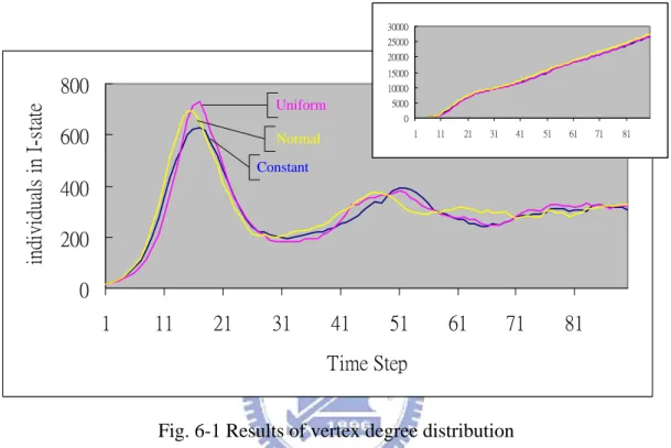
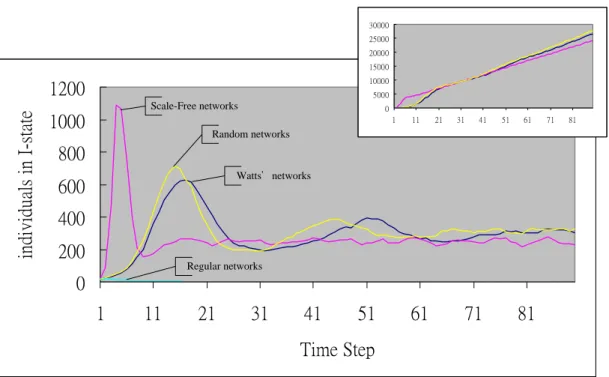
(25) vertex degree be normal distribution to display much normal people and fewer others. Except that, we would not configure this information in scale-free networks and random networks for keeping the particular property among them.. 30000 25000 20000 15000. individuals in I-state. 800. 10000 5000. Uniform. 0. 600. 1. Normal. 11. 21. 31. 41. 51. 61. 71. 81. Constant. 400 200 0 1. 11. 21. 31. 41. 51. 61. 71. 81. Time Step Fig. 6-1 Results of vertex degree distribution Contrary to our prediction, the results revealed that different ways for generating small-world networks would not affect the simulation what meant we would not consider the effect of social-thinking because of its little effects (Figure 6-1). We found that the first hill height, appearance time, and duration were all similar. Even the variances of total number of infectious individuals were much closed. These showed that although the shortcut-distribution was different, it would cause the infections in another area if there were sufficient opportunities for diseases or rumors transferring to the distant places, such that we would use the original small-world networks (constant probability) in the experiments below. However, there was essential difference among different models, such as random networks and scale-free networks (figure 6-2).. 18.

(26) 30000 25000 20000 15000 10000. individuals in I-state. 1200. 5000. Scale-Free networks. 1000. 0 1. 11. 21. 31. 41. 51. 61. 71. 81. Random networks. 800 Watts＇networks. 600 400 200. Regular networks. 0 1. 11. 21. 31. 41. 51. 61. 71. 81. Time Step. Fig. 6-2 Results of network structures analysis Random networks totally lost the clustering effect, so that the disease or the rumors would not be sustained in local area. But the simulation results revealed that the random network was similar to the small-world network, it was because we only connected 4 nearest neighbors for all individuals in 2-D lattice without sufficient clustering property. Besides no clustering effect, scale-free networks with power-law of vertex degree caused the more strange results than random networks. When the individual with high vertex degree was infected, then the number of individuals with I-state became the maximum very quickly, because of the highest probability for spreading disease occurred, that the individuals connected to the hub-nodes with high vertex degree called danger-groups. Such that the first hill appear earlier than other network models, and its duration was shorter too. On the other hand, we could find that the total number of infectious individuals increased with high-speed at beginning in scale-free networks. This circumstance was certainly different from other networks.. 19.

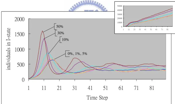
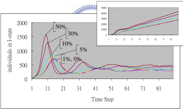
(27) 6.2 Weak Individual Proportions In this experiment we looked at the influence of the proportion of heterogeneous individuals. For instance, in some developed cities, most people are not easily infected by disease. But in backward countries, resistance against disease of people is quite not enough.. As described above, we checked the influence of that by doubling the chances of heterogeneous individuals becoming infected, and investigated the results when the proportions of heterogeneous individuals were set at 0, 1, 5, 10, 30, and 50 percent.. 50000 40000 30000. individuals in I-state. 2000. 20000 10000. 50%. 1500. 0 1. 11. 21. 31. 41. 51. 61. 71. 81. 30% 10%. 1000. 0%, 1%, 5%. 500 0 1. 11. 21. 31. 41. 51. 61. 71. 81. Time Step Fig. 6-3 Weak individual proportion in Watts’ networks Results are shown in Figure 6-5. We found that the higher the proportion of heterogeneous individuals, the earlier the appearance of the first hill and the higher the value of the top spot. Besides, according to the results and the variance of total number of infectious individuals, we could see there was not obvious variance at low. 20.

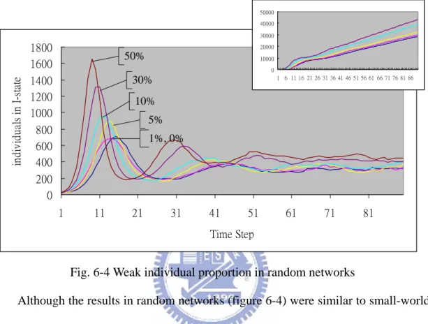
(28) weak proportion changes. We therefore suggest that the higher proportion of heterogeneous individuals in Watts’ networks is a significant factor.. 50000 40000. individuals in I-state. 30000. 1800 1600 1400 1200 1000. 20000. 50%. 10000 0 1 6 11 16 21 26 31 36 41 46 51 56 61 66 71 76 81 86. 30% 10% 5%. 800 600 400. 1%, 0%. 200 0 1. 11. 21. 31. 41. 51. 61. 71. 81. Time Step. Fig. 6-4 Weak individual proportion in random networks Although the results in random networks (figure 6-4) were similar to small-world networks, the epidemic propagation was slower without clustering.. 30000 25000 20000 15000. individuals in I-state. 2000. 10000. 50%. 5000 0 1. 30%. 1500. 11. 21. 31. 41. 51. 61. 10% 5%. 1000. 1% 0%. 500 0 1. 11. 21. 31. 41. 51. Time Step. 21. 61. 71. 81. 71. 81.

(29) Fig. 6-5 Weak individual proportion in scale-free networks In scale-free networks, more heterogeneous individuals and the higher the value of the top spot. Besides, deserve to mention that the first hill appeared at the same time whatever the proportion of heterogeneous individuals were. That is because of the structure of scale-free networks. Entire model is almost connected by hub-nodes, such that the danger area may be influenced when hub-nodes are infectious. As the results, we found that the proportion of heterogeneous individuals could influence the ill population, but never change the epidemic propagation restricted by network’s topologies.. 6.3 Distribution Patterns of Weak Individuals Follows is the investigation of distribution of heterogeneous individuals. Imaging the proportion of heterogeneous individuals between a developed city with shantytown and a normal city may be similar, but the distribution of these weak individuals causes the main difference. For scale-free networks and random networks, without nearest-neighbor links, that is no meaning of discussion on distribution of weak individuals although the heterogeneous individuals clustered together in the models. Therefore, we just investigated this problem in small-world networks.. 22.

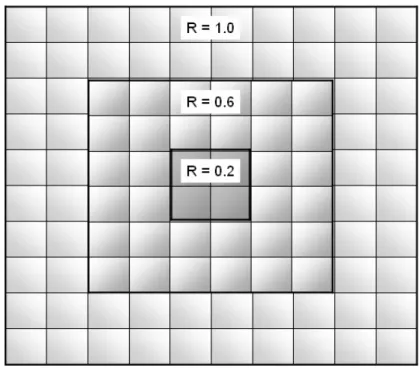
(30) Fig. 6-6 the radius representation In this experiment, we set the heterogeneous individuals at 1%, and used the parameter R representing the radius of distribution, and R would be 0, 0.2, 0.4, 0.6, 0.8, and 1.0. As shown in figure 6-6, all heterogeneous were clustered together while R was set to 0, and they were randomly being the entire model when R was 1.. 30000 25000. individuals in I-state. 20000 15000. 800 700 600 500 400 300 200 100 0. 10000 5000 0 1. 11. 21. 31. 41. 51. 61. 71. 81. 0, 0.2, 0.4, 0.6, 0.8, 1.0. 1. 11. 21. 31. 41. 51. 61. 71. 81. Time Step. Fig. 6-7 Distribution patterns of weak individual in small-world networks 23.

(31) As the results, we found that no matter how heterogeneous individuals scattered in small-world networks, it would not be a problem in epidemic simulations, what we said was an insensitive condition.. 6.4 Familiar pairs and One-way channels Proportions Then, we would look at the differences of weights and directions between nodes among the model. For instance, the interaction may be stronger between closed friends than others, and high frequency of contacts may cause more probability of infection of disease; and further, some epidemic sources may just infect others without being influenced, such that some links of them are one-way spreading. By these reasons, we analyzed the situations when randomly doubled some edges’ weight which cause double chance of infection or made some edges being one-way which spreading in only one direction, which we called heterogeneous channels.. As the experiment 2, we investigated the results when the proportions of double weighted channels were set at 0, 1, 5, 10, 30, and 50 percent.. 24.

(32) 50000. individuals in I-state. 40000 30000. 1600 1400 1200 1000 800 600 400 200 0. 50%. 20000 10000. 30% 10% 5%. 0 1. 11. 21. 31. 41. 51. 61. 71. 81. 1%. 0%. 1. 11. 21. 31. 41. 51. 61. 71. 81. Time Step. Fig. 6-8 Small-world networks 50000 40000 30000. individuals in I-state. 2000. 20000. 50%. 10000. 30%. 1500. 0 1. 11. 21. 31. 41. 51. 61. 10% 5%. 1000. 1%, 0% 500 0 1. 11. 21. 31. 41. 51. Time Step Fig. 6-9 Random networks. 25. 61. 71. 81. 71. 81.

(33) 35000 30000 25000. Individuals in I-state. 2000. 20000 15000 10000. 50% 30% 10% 5% 1%. 1500 1000 500. 5000 0 1. 11. 21. 31. 41. 51. 61. 71. 81. 0%. 0 1. 11. 21. 31. 41. 51. 61. 71. 81. Time Step. Fig. 6-10 Scale-free networks The results told us that more double weighted channels were set, more infectious people and earlier the first hill appeared.. And the discussion about directions of channels, we made 0, 1, 5, 10, 30, and 50 percent channels were set as one-way. 30000 25000. individuals in I-state. 20000 15000. 700 600 500 400 300 200 100 0. 10000. 0%. 5000 0. 1% 5% 10%. 30% 1. 11. 21. 31. 1. 11. 21. 31. 41. 51. 61. 50% 41. 51. 61. Time Step Fig. 6-11 Small-world networks 26. 71. 81. 71. 81.

(34) 30000 25000 20000 15000. Individuals in I-state. 800. 10000. 0%. 600. 5000 0. 1% 5% 10%. 400. 1. 11. 21. 31. 41. 51. 61. 71. 81. 200. 30%. 0 1. 11. 21. 50% 31. 41. 51. 61. 71. 81. Time Step. Fig. 6-12 Random networks 30000 25000 20000. individuals in I-state. 1500. 15000. 0%. 10000 5000. 1% 1000. 0 1. 5%. 11. 21. 31. 41. 51. 61. 71. 81. 30% 10% 50%. 500 0 1. 11. 21. 31. 41. 51. 61. 71. 81. Time Step Fig. 6-13 Scale-free networks Although these results showed that more one-way channels less efficiency in epidemic simulation, this factor would not affect the simulation very much at low percent of one-way channels. Therefore, we have to configure this factor carefully while many one-way channels are needed.. 27.

(35) 6.5 Distribution Patterns of Familiar pairs In this section we would focus on weighted edge distribution in the small-world network only. In our daily life, we had the better relationship with our family or neighbors, such that the double weighted edges might all appear in the nearest-neighbor links instead of double weighted edges randomly. By this reason, we would not discuss this issue in scale-free networks and random networks, which without nearest-neighbor links. We took two parts A and B into the experiment. A part meant the double weighted edges were distributed randomly in the network model, and B part meant the double weighted edges were all in the nearest-neighbor links. Then as the experiment 4, we looked at the difference of double weighted edges were set at 1, 5, 10, 30, and 50. Individuals in I-state. percent.. 1600 1400 1200 1000 800 600 400 200 0. 50% A, B. A: randomly double the weight of edges B: double the weight of nearest neighbor links. 30% A, B 10% A, B 5% A, B 1% A, B. 1. 11. 21. 31. 41. 51. 61. 71. 81. Time Step Fig. 6-14 Distribution pattern of familiar pairs in small-world networks Results from this experiment are shown in Figure 6-14. The similarity of the curves leads us to suggest that the influence of the pattern of scattered heterogeneous. 28.

(36) individuals is not significant.. 29.

(37) 7 Conclusion Summarizing all results, we classified the experiments into 3 types below, network-structures,. sensitive. information,. and. insensitive. information.. Network-structures information means that we have to determine what model is needed depending on various simulations. As mentioned above, we used scale-free networks for discussion of propagation of sexual disease, and used small-world networks for spreading of rumors. Besides, we could find that there was no significant difference between random networks and small-world networks with level one von Neumann Neighborhood, because of the lower clustering coefficient. The sensitive information indicates that the parameters of epidemic simulations which might change the infectious power. Take experiment 2 for example, without nearest-neighbor links, scale-free networks and random networks are constructed by shortcuts, such that the number of shortcuts may influence the simulation so much. Besides, in experiment 3, more heterogeneous individuals, weaker the whole society, and the influence of disease is larger. The different weighted channels are also the sensitive condition by affecting the efficiency between nodes. Say, these are all count in intensity information, and we have to configure them carefully. Finally, insensitive information is pointing to the parameters which are side issues in epidemic experiments. As the experiment 4, the efficiency of epidemic simulation was almost equal no matter what distributions of heterogeneous individuals were configured. And the experiment 6, we configured the double weighted edge by two different ways, but the simulation results were similar. Such the insensitive information can be ignored or configured arbitrarily.. 30.

(38) Appendix A 複雜網路本論文使用二維的細胞自動機來做為模擬平台。初始狀態除了規則網路以及小世界網路兩個有跟周圍四個鄰居連結之外，無尺度網路與隨機網路則都是呈現所有個體孤立的情況。接著在挑選個體對來增加捷徑方面，我們賦予個體一個新的權重參數 d(v)以便計算此個體將要被挑選出來增加捷徑的機率，挑選機率如下： P (v i ) =. d (v i ) ∑ d (v ). v∈V ( G ). 因此權重參數越高的個體，越容易被挑選出來與其他個體配對增加捷徑。然而為了不破壞無尺度網路以及隨機網路的網路拓墣，我們不特別對這兩種網路模型設定權重參數，然無尺度網路的權重參數則是按照其建構演算法般的自然增加。. 31.

(39) 規則網路與小世界網路建構流程圖如下： Start. For all individuals Vi in 2-D lattice Connect to 4 nearest neighbors Regular Network Set d(v) for all nodes. End. Determine the number of shortcuts. Yes. Pick nodes Va by its probability P(Va) Pick nodes Vb by its probability P(Vb). No Is_linked(a,b) No Link(a,b). Is shortcuts number enough. Yes Small-world Network. End. Fig. A-1 規則網路與小世界網路. 32.

(40) 隨機網路：. Start. All individuals in 2-D lattice are isolated. Determine the number of shortcuts. Yes. Pick two nodes a, b randomly. No Is_linked(a,b) No Link(a,b). Is shortcuts number enough. Yes Random Network. End Fig. A-2 隨機網路. 33.

(41) 無尺度網路： Start. All individuals in 2-D lattice are isolated All d(V) are configured to 1. Determine the number of shortcuts. Yes. Pick nodes Va by its probability P(Va) Pick nodes Vb by its probability P(Vb). No Is_linked(a,b) No Link(a,b) Increase d(Va) by 1 Increase d(Vb) by 1. Is shortcuts number enough. Yes Scale-Free Network. End. Fig. A-3 無尺度網路. 34.

(42) 而觀察各網路模型的節點分支度可發現，本論文所使用的三種小世界網路模型經過設定各節點的權重參數後得到的節點分支度分佈的確如我們所要，另外隨機網路當然呈現完全隨機的樣子，而無尺度網路也遵照最特殊的冪次定律來呈現他的分支度分佈。. 35.

(43) Appendix B 傳播問題建模傳播問題主要是指傳播者透過傳播途徑使接受者受到影響而改變。以流行病傳染為例，一般病人為傳播者透過直接接觸或是空氣傳染等途徑，使得正常人受到感染而成為病人。再以信仰傳播為例，傳教士為傳播者透過口頭傳教或是書報雜誌等傳播途徑使得一些人受到感招而信教。因此可以說傳播問題主要是需由傳播者、傳播途徑以及接受者三個部份所組成。在本論文中將使用各種社會網路模型來當作傳播問題模擬平台，由於不同性質的傳播問題所適用的網路模型都有所差異，因此無論是無尺度網路，小世界網路甚至是簡化的隨機網路都將在本研究中討論，而其中的隨機網路與規則網路則主要是做個比較，可以看看結構上的差異會造成多少不同的結果。另一方面本論文將使用 SIR 模型來模擬個體狀態改變的動態，使得互動過程呈現出傳播者透過網路模型上的連結來當作傳播途徑以達到影響並改變接受者的效果。. 檢視個體的狀態改變可以發現，當一個 Susceptible 個體經過連結與 Infectious 個體互動的過程，將有一個機率會把本身的狀態從 S 轉變成 I，稱之為，而隨著時間的經過，Infectious 個體將會以的機率被設定成移除或痊癒，若是個體形成痊癒狀態則因為產生抗體而比 Susceptible 個體來的不易被感染。以 SIR 模型來討論疾病傳染是較常被使用以及易被接受的，而文化的傳播或謠言擴散是否也能用相同的模型來做模擬呢？想像在選舉前的拉票動作，某個候選人在初始的狀況下擁有一些擁護者支持這個候選人的政見，假設這些擁護者為 Infectious 狀態，即是被候選人的政治魅力給感染了；而這些擁護者將會在親朋好友之間替這個候選人的政見做宣傳，因此也許有些機率讓原本沒有支持特定候選人的朋友 Susceptible 轉而支持相同的候選人；但是即使已經變成擁護者，仍. 36.

(44) 有特定的機率去相信一些所支持候選人的負面消息而放棄支持立場 Remove。. 融合 SIR 模型與複雜網路就成了本論文探討傳播問題所使用的平台了。檢視傳播問題架構流程圖(圖 B-2)可以發現個體間的互動需要透過人際關係網路的連結而非個體獨立且隨機的改變狀態，以此模型來探討傳播問題更能貼近真實世界，因此近來討論傳播問題的相關研究都使用類似的模型，本論文也使用此流程探討各種區域資訊的差異所造成的影響。. 37.

(45) 實驗流程圖： Start. Generate Network Model. Apply Local Information. Time Step Start. Next Individual. Interacts with all neighbors. No Last Individual?. Yes Update all individuals states. Limit of Time Step?. Yes End. Fig. B-2 實驗流程圖 38. No.

(46) Reference [1] EDELETEIN-KESHET L, 1988, “Mathematical Models in Biology,” Random House, New York. [2] Jørgensen, E., T.A. Søllested and N. Toft, 2000, “Evaluation of SIR epidemic models in slaughter pig units using Monte Carlo simulation, ”International Symposium on Pig Herd Management Modelisation, Lleida, Spain, September 18-20. [3] X. F. Wang and G. Chen, “Complex Networks: Small-World, Scale-Free and Beyond,” IEEE Circuits and Systems Magazine, First Quarter, pp. 6-20, 2003. [4] C. Y. Huang, C. T. Sun, J. L. Hsieh, and H. Lin, “Simulating SARS: Small-World Epidemiological Modeling and Public Health Policy Assessments,” Journal of Artificial Societies and Social Simulation, 7(4), http://jasss.soc.surrey.ac.uk/7/4/2.html, 2004. [5] F. Liljeros, CR. Edling, L. Amaral, HE. Stanley, and Y. Aberg, “The web of human sexual contacts,” Nature 411, 907-908, 2001. [6] Dami´an H. Zanette, “Critical behavior of propagation on small-world networks,” http://arxiv.org/abs/cond-mat/0105596, 2001. [7] H. C. Lin, “Influence of Local Information on Social Simulation under Small-World Model” (2004) [8] D. J. Watts and S. H. Strogatz, “Collective dynamics of ‘small-world’ networks,” Nature, vol. 393, 1998, pp.440-442. [9] S. Milgram, “The small world probe,” Psychology Today, vol. 2, 1967, pp.60-67 [10] M. E. J. Newman, “Models of the Small World: A Review,” Journal of Statistical Physics, 101, pp. 819-841, 2000. [11] P. Erdös and A. Rényi, “On the evolution of random graphs.” Publ. Math. Inst. Hung. Acad. Sci., vol. 5, pp.17-60, 1959. 39.

(47) [12] D. J. Watts and S. H. Strogatz, 1998, “Collective Dynamics of ‘Small-world’ Networks,” Nature, 393(6684), pp. 440-442. [13] M. E. J. Newman and D. J. Watts, “Renormalization group analysis of the small-world network model,” Physics Letters A, vol. 263, pp. 341-346, 1999. [14] A-L. Barabási and R. Albert, 1999, “Emergence of Scaling in Random Networks,” Science, 286(5439), pp. 509-512. [15] A-L. Barabási, R. Albert and H. Jeong, 1999, “Mean-field Theory for Scale-Free Random Networks,” Physics A, 272, pp. 173-187. [16] R. Albert and A-L. Barabási, 2002, “Statistical Mechanics of Complex Networks,” Review of Modern Physics, 74, pp. 47-91. [17] W. O. Kermack and A. G. McKendrick, “Contributions to the Mathematical Theory of Epidemics,” Proceedings of the Royal Society of London, Series A, 115, pp. 700-721. [18] Y. Moreno, R. Pastor-Satorras, and A. Vespignani, 2002, “Epidemic outbreaks in complex heterogeneous networks,” European Physical Journal B, 26(4), pp. 521-529,. [19] R. Pastor-Satorras, and A. Vespignani, 2001, “Epidemic spreading in Scale-Free Networks,” Physical Review Letter, 86, pp. 3200-3203. [20] M. E. J. Newman, 2002, “Spread of epidemic disease on networks,” Physical Review E, 66 (1 Pt 2). 016128.. 40.

(48)