國
立
交
通
大
學
資訊科學與工程研究所
碩
士
論
文
網格環境中支援工作流程應用程式之線上即時
排
程
方
法
Online Scheduling of Workflow Applications in a Grid
Environment
研 究 生:許志強
指導教授:王豐堅 教授
網格環境中支援工作流程應用程式之線上即時排程方法
Online Scheduling of Workflow Applications in a Grid Environment
研 究 生:許志強 Student:Chih-Chiang Hsu
指導教授:王豐堅 Advisor:Feng-Jian Wang
國 立 交 通 大 學
資 訊 科 學 與 工 程 研 究 所
碩 士 論 文
A ThesisSubmitted to Institute of Computer Science and Engineering College of Computer Science
National Chiao Tung University in partial Fulfillment of the Requirements
for the Degree of Master
in
Computer Science September 2009
Hsinchu, Taiwan, Republic of China
I
網格環境中支援工作流程應用程式之線上即時
排程方法
研究生: 許志強 指導教授: 王豐堅 博士 國立交通大學 資訊科學與工程研究所 新竹市大學路 1001 號 碩士論文摘要
在網格環境中對工作流程應用程式排程是個很大的挑戰,因為這類型的問題 是屬於 NP-complete。對於這類型問題,現今已經有許多探索式的方法被提出, 然而大部份都著重在排程單一個工作流程應用程式。近幾年來,有許多的研究致 力於處理並行或線上的工作流程,但在每個工作需要多顆處理器的情況這些研究 沒辦法處理,本文中,我們提出了一個 OWM 方法,OWM 對線上工作流程可以有效 的做排程。為了解決當工作需要多顆處理器所面臨的問題,我們加入解決這類問 題的一些有名方法到 OWM 中,如:first fit,conservative backfilling,easy backfilling。根據模擬實驗,數據顯示我們所提出的 OWM 表現的比其他方法還 要 傑 出 ; 而 在 工 作 需 要 多 顆 處 理 器 的 情 況 下 , OWM(FCFS) 表 現 的 幾 乎 和 OWM(conservative)一樣並且 OWM(FCFS)表現的比 OWM(easy)和 OWM(first fit) 還要來的好。關鍵字: 線上工作流程,不循環有向圖,工作圖,工作流程排程,工作排程,異 質系統,網格計算,工作配置,資料平行,回填機制。
II
Online Scheduling of Workflow Applications in
a Grid Environment
Student: Chih-Chiang Hsu Advisor: Feng-Jian Wang
Institute of Computer Science and Engineering
National Chiao Tung University
1001 University Road, Hsinchu, Taiwan 300, ROC
Abstract
Scheduling workflow applications in a Grid environment is a great challenge,
because it is NP-complete problem. Many heuristic methods are presented, but most
of them work in the domain of single workflow application. In recent years, there are
several heuristic methods presented to deal with concurrent workflows or online
workflows, but they do not work with workflows composed of data-parallel tasks. In
the thesis, we present an approach for dealing with online workflows, which is named
Online Workflow Management (OWM). For dealing with data-parallel problems,
well-known approaches, e.g., first fit, conservative backfilling and easy backfilling
are added into OWM. The experiments show that OWM outperforms other two
methods in various workloads. For workflows composed of data-parallel tasks, the
experiments show that OWM(FCFS) is almost equal OWM(conservative), and
outperforms OWM(easy) and OWM(first fit).
Keywords: Online Workflows, DAG, Task Graph, Workflow Scheduling, Task Scheduling, Heterogeneous Systems, Grid Computing, Task Allocation, Data Parallel
III
誌謝
本篇論文得以順利完成,最主要要感謝我的指導教授王豐堅老師,在交大這 兩年期間傳道授業解惑讓我在軟體工程、工作流程以及網格計算領域能夠深入了 解,並且獲得許多知識以及經驗。另外,也十分感謝口試委員鍾葉青博士、張西 亞博士以及黃國展博士的寶貴意見,得以補足我論文的不足之處。 其次,要感謝實驗室的學長姐、同學及學弟們這兩年來的砥礪、照顧以及指 導。尤其是黃國展學長給于的許多寶貴意見及指導,讓我在研究上遇到瓶頸時得 以順利克服,不管是專業的知識、研究技巧以及文章寫作都讓我受益良多,因為 有學長不厭其煩的指導,本篇論文才得以順利完成。當然還有一群總是默默支持 我的朋友們,在我低潮時給于我加油及鼓勵,謝謝你們。 最後,我要感謝我最親愛的家人們,因為有你們支持、陪伴,才讓我有繼續 前進的動力,本篇論文才得以順利完成,謝謝我最親愛的家人們,本篇論文獻給 你們。IV
Table of Contents
摘要………..Ⅰ
Abstract……….Ⅱ
誌謝………..Ⅲ
Table of Contents………..Ⅳ
List of Tables………Ⅵ
List of Figures………...Ⅶ
Chapter 1 Introduction……….1
Chapter 2 Related Work………...3
2.1 Workflow Scheduling Algorithms for Grid Computing
……… ..3
2.2 Static Workflow Scheduling Algorithms
...5
2.3 Scheduling Concurrent Workflows in Grid Environments
...9
2.4 Scheduling Online Workflows in Grid Environments
………10
2.5 Scheduling Mixed Parallel Workflows in Grid Environments
……….10
Chapter 3 Software Simulator for Workflow Scheduling………..12
3.1 Data Components in the Simulator
………12
3.2 Classes in the Simulator
………...14
3.3 Simulation Process
……….23
Chapter 4 Online Workflow Management in a Grid Environment……28
4.1 Structure of Online Workflow Management
………28
4.2 Online Workflow Management (OWM)
……….30
V
4.2.2 Critical Path Workflow Scheduling (CPWS)
………30
4.2.3 Adaptive Allocation (AA)
……….33
Chapter 5 Experimental Results………37
5.1 Performance Metrics
………...37
5.2 Experimental Results for Workflows Composed of Single-Processor Tasks
..38
5.2.1 Difference between RANK_HYBD, Fairness_Dynamic and OWM
…38
5.2.2 Experimental Setup……….39
5.2.3 Results Analyses
……….40
5.3 Experimental Results for Workflows Composed of Data-Parallel Tasks
…...52
5.3.1 Experimental Setup
……….52
5.3.2 Results Analyses
……….54
Chapter 6 Conclusion and Future Work………..…………..57
Appendix………..58
VI
List of Tables
Table 3-1 DAG_Generator class………..14
Table 3-2 EventNode class………...16
Table 3-3 EventType enumeration………16
Table 3-4 EventQueue class……….17
Table 3-5 WaitQueueNode class………...19
Table 3-6 WaitQueue class………...20
Table 3-7 WorkflowScheduling class………...21
VII
List of Figures
Figure 2-1 A taxonomy of workflow scheduling algorithms……….3
Figure 2-2 An example of static scheduling………...4
Figure 2-3 A taxonomy of static workflow scheduling algorithms………5
Figure 2-4 An example of a list-based heuristic……….6
Figure 2-5 An example of a clustering-based heuristic………..7
Figure 3-1 A Grid Environment………...13
Figure 3-2 An example of EventQueue………18
Figure 4-1 Online Workflow Management (OWM)………29
Figure 4-2 An example of SWS ………..32
Figure 4-3 An example of CPWS……….32
Figure 5-1 The difference between RANK_HYBD, Fairness_Dynamic and OWM...38
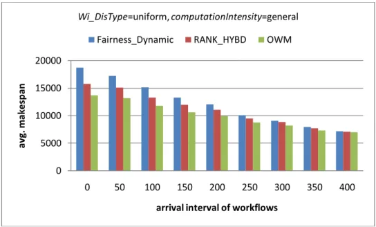
Figure 5-2 Results of different mean arrival intervals for average makespan……….41
Figure 5-3 Results of different mean arrival intervals for average SLR………..41
Figure 5-4 Results of different mean arrival intervals for win (%)………..42
Figure 5-5 Results of different computation intensity for average makespan with a uniform distribution of tasks’ computation cost………...43
Figure 5-6 Results of different computation intensity for average SLR with a uniform distribution of tasks’ computation cost………...44
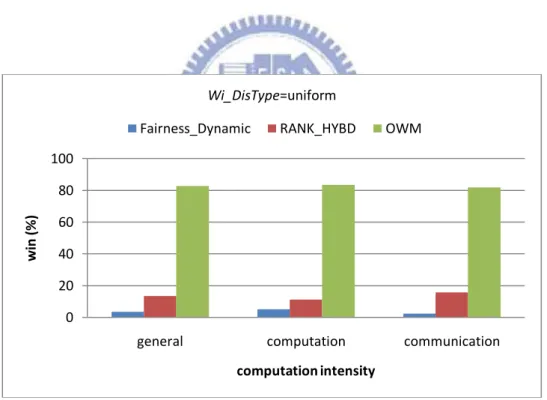
Figure 5-7 Results of different computation intensity for win (%) with a uniform distribution of tasks’ computation cost……….44
Figure 5-8 Results of different computation intensity for average makespan with an exponential distribution of tasks’ computation cost………...45
VIII
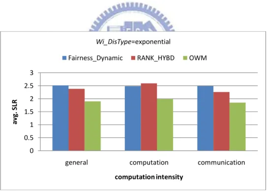
Figure 5-9 Results of different computation intensity for average SLR with an
exponential distribution of tasks’ computation cost……….45
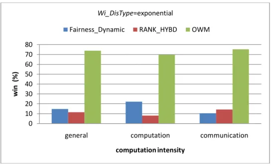
Figure 5-10 Results of different computation intensity for win (%) with an
exponential distribution of tasks’ computation cost……….46
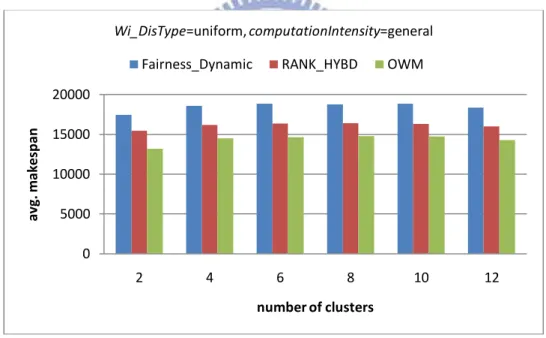
Figure 5-11 Results of different number of clusters for average Makespan…………47
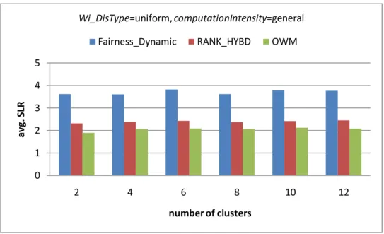
Figure 5-12 Results of different number of clusters for average SLR……….48
Figure 5-13 Results of different number of clusters for win (%)……….48
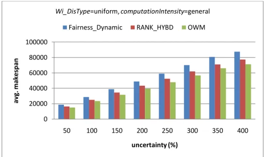
Figure 5-14 Results of inaccurate execution estimates for average makespan………50
Figure 5-15 Results of inaccurate execution estimates for average SLR……….50
Figure 5-16 Results of inaccurate execution estimates for win (%)……….51
Figure 5-17 The processes in OWM(FCFS), OWM(conservative), OWM(easy) and
OWM(first fit)………..52
Figure 5-18 Results of different computation intensity for average makespan
with (uniform, min, uniform)………...55
Figure 5-19 Results of different computation intensit y for average SLR
with (uniform, min, uniform).………...56
F ig u r e 5-2 0 R e su lt s o f d iffe r e nt co mp ut at io n int e ns it y fo r w in ( % )
with (uniform, min, uniform)………...56
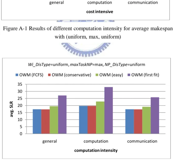
Figure A-1 Results of different computation intensity for average makespan
with (uniform, max, uniform)………58
Figure A-2 Result s of different computation intensit y for average SLR
with (uniform, max, uniform)………58
F ig u r e A- 3 R e s u lt s o f d iffe r e nt co mp u t at io n int e ns it y fo r w in ( % )
with (uniform, max, uniform)………59
Figure A-4 Results of different computation intensity for average makespan
IX
Figure A-5 Result s of different computation intensit y for average SLR
with (uniform, max, exponential)………..60
F ig u r e A- 6 R e s u lt s o f d iffe r e nt co mp u t at io n int e ns it y fo r w in ( % )
with (uniform, max, exponential)………...60
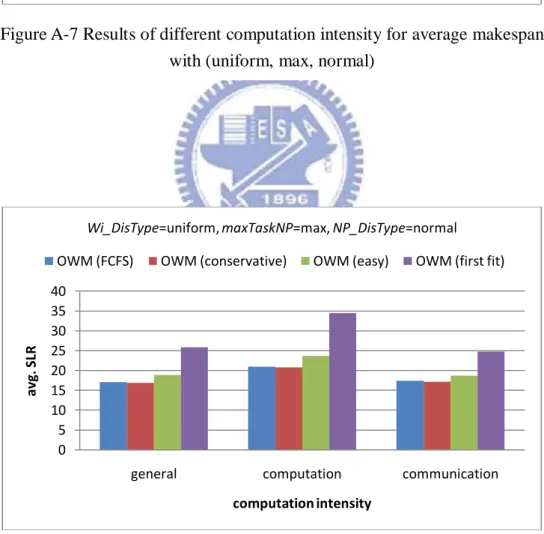
Figure A-7 Results of different computation intensity for average makespan
with (uniform, max, normal)………..61
Figure A-8 Result s of different computation intensit y for average SLR
with (uniform, max, normal)………..61
F ig u r e A- 9 R e s u lt s o f d iffe r e nt co mp u t at io n int e ns it y fo r w in ( % )
with (uniform, max, normal)………..62
Figure A-10 Results of different computation intensity for average makespan
with (uniform, half, uniform)………...62
Figure A-11 Results of different computation intensity for average SLR
with (uniform, half, uniform)………...63
Fig ur e A- 12 Re s u lt s o f d iffe re nt co mpu t at io n int e ns it y fo r w in (%)
with (uniform, half, uniform)………...63
Figure A-13 Results of different computation intensity for average makespan
with (uniform, half, exponential)……….64
Figure A-14 Results of different computation intensity for average SLR
with (uniform, half, exponential)……….64
Fig ur e A- 15 Re s u lt s o f d iffe re nt co mpu t at io n int e ns it y fo r w in (%)
with (uniform, half, exponential)……….65
Figure A-16 Results of different computation intensity for average makespan
with (uniform, half, normal)……….65
Figure A-17 Results of different computation intensity for average SLR
X
Fig ur e A- 18 Re s u lt s o f d iffe re nt co mpu t at io n int e ns it y fo r w in (%)
with (uniform, half, normal)……….66
Figure A-19 Results of different computation intensity for average makespan
with (uniform, min, exponential)……….……….67
Figure A-20 Results of different computation intensity for average SLR
with (uniform, min, exponential)……….67
Fig ur e A- 21 Re s u lt s o f d iffe re nt co mpu t at io n int e ns it y fo r w in (%)
with (uniform, min, exponential)……….68
Figure A-22 Results of different computation intensity for average makespan
with (uniform, min, normal)……….68
Figure A-23 Results of different computation intensity for average SLR
with (uniform, min, normal)……….69
Fig ur e A- 24 Re s u lt s o f d iffe re nt co mpu t at io n int e ns it y fo r w in (%)
with (uniform, min, normal)……….69
Figure A-25 Results of different computation intensity for average makespan
with (exponential, max, uniform)……….70
Figure A-26 Results of different computation intensity for average SLR
with (exponential, max, uniform)……….70
Fig ur e A- 27 Re s u lt s o f d iffe re nt co mpu t at io n int e ns it y fo r w in (%)
with (exponential, max, uniform)……….71
Figure A-28 Results of different computation intensity for average makespan
with (exponential, max, exponential)………...71
Figure A-29 Results of different computation intensity for average SLR
with (exponential, max, exponential)………...72
Fig ur e A- 30 Re s u lt s o f d iffe re nt co mpu t at io n int e ns it y fo r w in (%)
XI
Figure A-31 Results of different computation intensity for average makespan
with (exponential, max, normal)………….………..73
Figure A-32 Results of different computation intensity for average SLR
with (exponential, max, normal)………..73
Fig ur e A- 33 Re s u lt s o f d iffe re nt co mpu t at io n int e ns it y fo r w in (%)
with (exponential, max, normal)………..74
Figure A-34 Results of different computation intensity for average makespan
with (exponential, half, uniform)……….74
Figure A-35 Results of different computation intensity for average SLR
with (exponential, half, uniform)……….75
Fig ur e A- 36 Re s u lt s o f d iffe re nt co mpu t at io n int e ns it y fo r w in (%)
with (exponential, half, uniform)……….75
Figure A-37 Results of different computation intensity for average makespan
with (exponential, half, exponential)………76
Figure A-38 Results of different computation intensity for average SLR
with (exponential, half, exponential)………76
Fig ur e A- 39 Re s u lt s o f d iffe re nt co mpu t at io n int e ns it y fo r w in (%)
with (exponential, half, exponential)………77
Figure A-40 Results of different computation intensity for average makespan
with (exponential, half, normal)……….………...77
Figure A-41 Results of different computation intensity for average SLR
with (exponential, half, normal)………...78
Fig ur e A- 42 Re s u lt s o f d iffe re nt co mpu t at io n int e ns it y fo r w in (%)
with (exponential, half, normal)………...78
Figure A-43 Results of different computation intensity for average makespan
XII
Figure A-44 Results of different computation intensity for average SLR
with (exponential, min, uniform)……….79
Fig ur e A- 45 Re s u lt s o f d iffe re nt co mpu t at io n int e ns it y fo r w in (%)
with (exponential, min, uniform)……….80
Figure A-46 Results of different computation intensity for average makespan
with (exponential, min, exponential)……….………80
Figure A-47 Results of different computation intensity for average SLR
with (exponential, min, exponential)………81
Fig ur e A- 48 Re s u lt s o f d iffe re nt co mpu t at io n int e ns it y fo r w in (%)
with (exponential, min, exponential)………81
Figure A-49 Results of different computation intensity for average makespan
with (exponential, min, normal)………….………...82
Figure A-50 Results of different computation intensity for average SLR
with (exponential, min, normal)………...82
Fig ur e A- 51 Re s u lt s o f d iffe re nt co mpu t at io n int e ns it y fo r w in (%)
1
Chapter 1 Introduction
Grid environments are an important platform for running high-performance and
distributed applications. Many large-scale scientific applications are usually
constructed as workflows due to large amounts of interrelated computation and
communication, e.g., Montage [29] and EMAN [30]. A Grid environment is
composed of widespread resources from different administrative domains. Miguel et
al. [33] indicates that a Grid environment usually has the characteristics: heterogeneity,
large scale and geographical distribution. Task scheduling in Grid is a NP-complete
problem [31] [32], therefore many heuristic methods have been proposed. The
workflow scheduling problem in Grid environments is a great challenge. In the past
years, there are many static heuristic methods proposed [3] [4] [5] [6] [7] [8] [9] [18]
[25]. They are designed in the domain of scheduling single workflow only.
Zhao et al. presented composition and fairness approaches [20] for scheduling
multiple workflows at the same time. T. N'takpe' et al. presented an approach [23] to
scheduling concurrent workflows composed of moldable tasks. However, all these
methods do not work with online workflows: i.e., multiple workflows occur at
different times. Z. Yu et al. [21] presented a planner-guided dynamic scheduling
approach for dealing with online workflows, but it doesn’t work with workflows
composed of data-parallel tasks (parallel tasks) of which each uses multiple
processors simultaneously for its execution.
In this thesis, we present a new approach called Online Workflow Management
(OWM). There are four processes in OWM: Critical Path Workflow Scheduling
(CPWS), Task Scheduling, Multi-Processor Task Rearrangement and Adaptive
2
scheduling and AA processes prioritize the tasks in the queue and assign the task with
highest priority to the processor for execution respectively. In data-parallel task
scheduling, there may be some scheduling holes which are formed when the free
processors are not enough for the first task in the queue. The multi-processor
rearrangement process works for dealing with scheduling holes to improve utilization.
The process includes first fit, easy backfilling [22], and conservative backfilling [22]
approaches.
To validate the advantages of the cooperation designed among these four
processes, task-waiting queue, event queue and workflows, we developed a Grid
simulator using a discrete-event based technique for experiments. Task-waiting queue
and event queue keep the tasks and events for processing. The Grid environment
consists of several simulated clusters of which each contains an amount of processors.
A workflow is represented by direct acyclic graph (DAG). Each experiment involves
20 runs, and each run has 100 unique DAGs on a Grid environment that contains 3
clusters each containing 30~50 processors respectively. Experimental results show
that OWM has better performance than RANK_HYBD [21] and Fairness_Dynamic
which extends the Fairness (F2) in [20] to handle online workflows. When workflows
composed of data-parallel tasks, the experimental results show that OWM(FCFS) is
almost equal to OWM(conservative), and outperforms OWM(easy) and OWM(first
fit).
The remainder of the thesis is organized as follows. Chapter 2 discusses related
work. Chapter 3 describes the software simulator for workflow scheduling. Chapter 4
presents the OWM approach for Grid environments. Chapter 5 presents the
3
Chapter 2 Related Work
In this chapter, we survey related algorithms in Grid environments. Section 2.1
describes workflow scheduling algorithms for Grid computing. Section 2.2 describes
static workflow scheduling algorithms. Section 2.3, 2.4, 2.5 describe concurrent
workflows, online workflow and mixed parallel workflows scheduling algorithms in
Grid environments respectively.
2.1 Workflow Scheduling Algorithms for Grid Computing
Workflow scheduling algorithms for Grid computing can be classified into two
groups [26] (Figure 2-1): static and dynamic.
In a static scheduling algorithm, the structure of workflow applications i.e., the
dependency of tasks, and the estimated cost are known in the very beginning. The
resource assignment of tasks is made before execution (Figure 2-2), and each
approach has its own policy of assignment. Static approaches are not adaptive to some
situations, e.g., one of the resources selected fails, or the real execution time on some
resources is longer than the estimated time. Unfortunately, these situations occur in a
great potential due to the nature of Grid environments. To alleviate this problem, there Figure 2-1 A taxonomy of workflow scheduling algorithms
4
are two approaches: task partitioning [10] and rescheduling [1] [11]. The former
partitions a workflow into multiple sub-workflows which are executed sequentially.
Instead of mapping entire workflow at one time, it allocates resources to tasks in one
sub-workflow each time. A sub-workflow mapping is started only after the previously
mapped sub-workflow starts the execution. The latter reschedule unexecuted tasks
when the Grid environment changes. H. Braun et al. compare eleven static heuristic
algorithms on heterogeneous distributed computing systems [2]. Figure 2-2 shows an
example of a static scheduling algorithm. Figure 2-2(a) shows an original workflow.
Figure 2-2(b) shows the resource mapping of tasks before execution: t1, t3 and t5 are
mapped to R1, and t2 and t4 are mapped to R2 .
Dynamic scheduling approaches perform task allocation as workflow
applications execute. When a task is ready to execute, it is submitted to waiting queue.
Dynamic scheduling mechanisms make a decision when the waiting queue has tasks
and there are free resources. Dynamic scheduling is usually applied when it is difficult
Figure 2-2 An example of static scheduling (a) an original workflow (b) the resource mapping of a workflow before execution
5
to estimate the costs of tasks, or when workflow applications may come at different
times (it is called online scheduling). For example, Z. Yu [21] proposed a
planner-guided scheduling strategy.
2.2 Static Workflow Scheduling Algorithms
Static workflow scheduling algorithms can be classified into two groups [17] as
shown in Figure 2-3: heuristic-based and meta-heuristic based.
Heuristic-based scheduling algorithms usually can be classified into five groups:
(1) list-based, (2) clustering-based, (3) duplication-based, (4) level-based, (5)
hybrid-based. A list-based heuristic approach maintains a list of all tasks of a
workflow application according to their priorities. The method schedules the tasks
based on the list. There are list-based heuristics proposed [3] [4] [5] [6] [7].
HEFT (Heterogeneous Earliest Finish Time) [7] is a well-known list-based Figure 2-3 A taxonomy of static workflow scheduling algorithms
6
scheduling algorithm in heterogeneous environments, and it is implemented in
ASKLON that is a workflow management system based on Grid computing [17]. In
recent years, many researches have been applied to modify HEFT in the
corresponding environments. Typical examples include HHS (Hybrid Scheduling
Algorithm) [18], M-HEFT (Mixed-Parallel HEFT) [19], Fairness Policy [20] ,
RANK_HYBD [21].
HEFT algorithm has two major phases: a task prioritizing phase and a processor
selection phase. The task prioritizing sets the priority of each task with an upward
rank value, ranku, which is based on mean computation and mean communication
costs. A higher ranku value gets a higher priority. The processor selection selects a
processor which has earliest estimated finish time of the task. Figure 2-4 shows an
example of a list-based heuristic, HEFT.
The main idea of clustering-based heuristic method is to reduce communication
delay by grouping the tasks of heavy communicating into the same labeled cluster. In
general, a clustering-based heuristic method has two phases: clustering and merging.
In the clustering phase, the original workflow application is partitioned into clusters,
and the merging phase merges the clusters so that the remaining number of clusters Figure 2-4 An example of a list-based heuristic
7
equals to the number of resources. There are various clustering-based heuristic
methods proposed [8]. Figure 2-5 shows an example of a clustering-based heuristic. In
figure 2-5, (a) represents an original workflow, and (b) shows the result of arranging
the tasks into three clusters {t1, t2, t7}, {t3, t4, t6}, {t5}. These three clusters {t1, t2,
t7}, {t3, t4, t6}, {t5} will be allocated to three resources respectively at run time.
A duplication-based heuristic method helps a task to transmit the data to the
resource of succeeding task(s) implicitly during its execution time. This may reduce
the communication cost from a task to a successor. Various duplication-based
heuristic methods are proposed [9].
A level-based heuristic method, i.e. LHBS (Levelized Heuristic Based
Scheduling) [25], divides the workflow into levels of independent tasks. Within each Figure 2-5 An example of a clustering-based heuristic (a) an original
8
level, LHBS can use Greedy, Min-Min, Min-Max, or Sufferage [2] heuristics to map
the tasks to resources. Both the GrADS [16] and Pegasus [27] schedulers use a
version of LHBS.
A Hybrid-based heuristic method, i.e., HHS (Hybrid Heuristic Scheduling) [18],
is a combination of list-based and level-based heuristic methods. HHS first computes
the levels as in LHBS, then the tasks in each level following the prioritized order used
by HEFT. The five static heuristic methods mentioned above are restricted to single
workflow.
Y. Zhang et al. [24] compare HEFT [7], LHBS [25], and HHS [18] in Grid
environments. They showed that list-based and hybrid-based heuristic methods are
effective in a Grid environment, outperforming the level-based heuristic. [15] also
shows that list-based heuristic method perform better than clustering-based and
duplication-based heuristic methods.
The meta-heuristic based scheduling algorithms produces an optimized
scheduling solution based on the performance of the entire workflow. Genetic
algorithms [13], simulated annealing [14], and GRASP (Greedy randomized adaptive
search) [12] are well-known meta-heuristic scheduling algorithms. Each task in the
workflow is assigned a priori to resources in order to minimize the makespan of the
whole workflow. However, the scheduling time in meta-heuristic scheduling
algorithms is significantly higher [16] [17] than heuristic-based algorithms.
J. Blythe et al. [16] compare the heuristic-based algorithm and the meta-heuristic
based algorithm. In the comparison, they select one algorithm to represent each
9
for the meta-heuristic based algorithm. The experiment results indicate both
approaches are similar for compute-intensive cases, but the meta-heuristic based
algorithm is better than the heuristic-based algorithm for data-intensive cases.
However, the time complexity of the meta-heuristic based algorithm grows more
rapidly than the heuristic-based algorithm if the workflow has more tasks.
2.3 Scheduling Concurrent Workflows in Grid Environments
In the past years, most works dealing with workflow scheduling were restricted
to single workflow application. Zhao et al. [20] envisaged a scenario that need to
schedule multiple workflow applications at the same time. They proposed two
approaches: composition approach and fairness approach.
(1) The composition approach merges multiple workflows into a single workflow
first. Then, two list scheduling heuristic methods, such as HEFT [7] and HHS
[18], can be used to schedule the merged workflow.
(2) The main idea of fairness approach is that when a task completes, it will
re-calculate the slowdown value of each workflow (or single workflow) against
other workflows and make a decision on which a workflow should be
considered next.
Moreover, the composition and the fairness approaches are static algorithms and
not feasible to deal with online workflow applications, i.e., multiple workflows come
10
2.4 Scheduling Online Workflows in Grid Environments
RANK_HYBD [21] is designed to deal with online workflow applications
submitted by different users at different times. The task scheduling approach of
RANK_HYBD sorts the tasks in waiting queue using the rules repeatedly.
1. If tasks in waiting queue come from multiple workflows, the tasks are sorted
in ascending order of their rank value (ranku) where ranku is described in
HEFT [7];
2. If all task are belong to the same workflow, the tasks are sorted in descending
order of their rank value (ranku).
However, the number of processors to be used by each task is limited to a single
processor. It is not feasible to deal with workflows composed of data-parallel tasks.
2.5 Scheduling Mixed Parallel Workflows in Grid Environments.
Parallel task scheduling can be classified into two modes: rigid and moldable.
The number of processors required by a rigid task is fixed. The number of processors
used in a moldable task is determined by some algorithms before each run.
T. N'takpe' et al. proposed mixed parallel applications on Heterogeneous
platforms [28]. This can be considered as an example of moldable mode. Mixed
parallelism is a combination of task parallelism and data parallelism where the former
indicates that an application has more than one task that can execute concurrently and
the latter means a task can run at different resources concurrently.
[28] is only suitable for a single workflow. T. N'takpe' et al. further developed an
approach to deal with concurrent mixed parallel applications [23]. Concurrent
scheduling for mixed parallel applications contains two steps: constrained resource
11
for each task. The number of processors is determined in this step. The latter
prioritizes tasks of workflows.
However, the approach in [23] is restricted to concurrent workflows. It is
12
Chapter 3 Software Simulator for Workflow
Scheduling
This chapter presents the software simulator that we developed for simulating the
workflow scheduling activities in a Grid environment. Section 3-1 describes data
components in the simulator. Section 3-2 describes classes used in the simulator and
section 3-3 presents simulation processes.
3.1 Data Components in the Simulator
Input Workload:
A workflow application is represented by a direct acyclic graph (DAG). A DAG
is defined as G = (V, E), where V is a set of nodes, each representing a task, and E is
the set of links, each representing the computation precedence order between two
tasks. For example, a link (x,y) ∈ E represents the precedence constraint that task tx
completes before task ty starts.
Global System Time (GST):
In a discrete-event based simulation, the simulator maintains a global timing
system which increments the time whenever an event is processed.
System Queues:
There are two system queues: an event queue and a waiting queue. They keep the
13
Grid Environment:
A Grid is composed of several clusters. A cluster contains an amount of
processors. The Grid is heterogeneous in that the processors at different clusters might
run at different speed. On the other hand, each cluster is homogeneous, consisting of
identical processors. The cost for a task includes computation and communication
costs where the former means the execution time, and the latter means the data
transfer time between processors. The computation cost of a task is the same for
different processors in the same cluster, but may be different in different clusters. The
communication cost between any two processors in the same cluster is set to be zero,
but not in different clusters. Figure 3-1 shows an example of a Grid environment in
our simulator. The processor speeds and network link speeds are homogeneous in the
same cluster, but they are heterogeneous between different clusters.
14
3.2 Classes in the Simulator
In this section, the classes used in the simulator are described including
DAG_Generator, EventNode, EventQueue, WaitQueueNode, WaitQueue,
WorkflowScheduling and Allocation classes.
DAG_Generator:
DAG_Generator is responsible for generating input workload consisting of a
sequence of DAGs in their arrival order. Table 3-1 shows an UML DAG_Generator
class. It contains 7 attributes, <Node, Shape, OutDegree, CCR, BRange, WDAG,
Cluster>, and 4 operations, <Generator(), ShapeGenerator(Node, Shape),
RelationGenerator(Node, OutDegree), CostGenerator(Node, BRange, WDAG, Cluster,
CCR)>.
The attributes and operations in DAG_Generator are described as following.
Attributes:
1. Node: the number of tasks in a DAG.
2. Shape: the shape of a DAG.
3. OutDegree: the maximum of out degree of tasks in a DAG.
4. CCR: communication cost to computation cost ratio.
5. BRange (β): distribution range of computation cost of tasks on processors. It is the heterogeneous factor for processor speeds. A high range indicates
15
significant differences in task’s computation costs among the processors and a
low range indicates that the expected execution time of a task is almost the
same on each processor.
6. WDAG: the average computation cost of a DAG.
7. Cluster: the number of clusters in a Grid environment.
Operations:
1. Generator(): randomly generates a DAG according to the 7 input parameters
mentioned above. It invokes ShapeGenerator(), RelationGenerator(),
CostGenerator() in turn.
2. ShapeGenerator(Node, Shape): generates the shape of a DAG using Node and
Shape parameters. The height (depth) of a DAG is randomly generated from a
uniform distribution with mean value equal to Node
Shape . The width for each level
is randomly generated from a uniform distribution with mean value equal to
Shape × Node . If 𝑠ℎ𝑎𝑝𝑒 ≫ 1 , it generates a shorter graph with high parallelism degree. Otherwise, if shape ≪ 1, it generates a longer graph with a low parallelism degree.
3. RelationGenerator(Node, OutDegree): generates the connect relation of a DAG
according to the input parameters Node and OutDegree defined above. Out
degree of each task is randomly generated from a uniform distribution with
range [1, OutDegree].
4. CostGenerator(Node, BRange, WDAG, Cluster, CCR): generates the
computation cost and the communication cost of a DAG. The average estimated
computation cost of each task tx, i.e., w is randomly generated from a x distribution ranged [1, 2 × WDAG]. The estimated computation cost of each
16
task tx on each cluster cy, i.e., wx,y is randomly generated from a uniform distribution with range:
wx × (1 −BRange 2 ) ≤ wx,y ≤ w × (1 +x BRange 2 )
EventNode:
EventQueue stores a set of EventNodes. Each EventNode contains 6 attributes,
<type, time, jobIndex, dagIndex, *pre, *next>. Table 3-2 shows EventNode class.
Attributes:
1. type: the type of an event. Table 3-3 shows EventType enumeration. There are two kinds of EventType: submit and end. Each event contains the attributes,
<jobIndex, dagIndex> uniquely identifying a job. When a submit event occurs,
a job <jobIndex, dagIndex> will be submitted to WaitQueue for scheduling and
allocation. When an end event occurs, a job <jobIndex, dagIndex> completes
successfully.
Table 3-2 EventNode class
17 2. time: the time that the event happens. 3. jobIndex: the index of a job.
4. dagIndex: the index of a dag.
5. *pre: a link pointing to the preceding EventNode. 6. *next: a link pointing to the next EventNode.
EventQueue:
EventQueue is composed of a sequence of EventNodes. There are 3 attributes,
<*front, *rear, eventQueueCount>, and 3 operations, <enQueue(EventNode),
deQueue(), isEmpty()> in EventQueue. Table 3-4 shows EventQueue class.
Attributes:
1. *front: points to the first EventNode in EventQueue.
2. *rear: points to the last EventNode in EventQueue.
Operations:
1. enQueue(EventNode): an operation that inserts an EventNode into
EventQueue.
2. deQueue(): an operation that removes and returns the first EventNode in
EventQueue.
18
3. isEmpty(): an operation that checks whether EventQueue is empty or not. If
EventQueue is empty, it returns true. Otherwise, it returns false.
Figure 3-2 shows an example of EventQueue. The EventNodes are sorted
according to their arrival time (EventNode.time). *fornt points to the first EventNode,
EventNode1, and *rear points to the last EventNode, EventNode5.
19
WaitQueueNode:
WaitQueueNode represents the elements stored in WaitQueue. There are 7
attributes, <jobIndex, dagIndex, np, ftown, ftmulti, rank, slowdown> in
WaitQueueNode. Table 3-5 shows WaitQueueNode class.
Attributes:
1. jobIndex: the index of a job.
2. dagIndex: the index of a dag.
3. np: the number of processors that the job <jobIndex, dagIndex> needs.
4. ftown: the finish time of the job <jobIndex, dagIndex>, when the DAG has the
whole processors for exclusive use. The detail of ftown is described in [20].
5. ftmulti: the finish time of the job <jobIndex, dagIndex>, when the DAG is
scheduled onto processors along with other workflow applications. The detail
of ftmulti is described in [20].
6. rank: the upward rank value ranku. ranku(ti) means the length of critical
path from task ti to the exit task. The detail of ranku is described in Chapter 4.
7. slowdown: the main idea of the slowdown value is defined as ftown / ftmulti. The
detail of slowdown is described in [20].
20
WaitQueue:
WaitQueue is composed of a sequence of WaitQueueNodes. On a submit event, a
new WaitQueueNode is created according to the EventNode, and is submitted to
WaitQueue by calling WaitQueue.enQueue (WaitQueueNode) operation. WaitQueue
has 2 attributes, <waitQueueCount, waitQueue[]>, and 10 operations,
<enQueue(WaitQueueNode), remove(WaitQueueNode), isEmpty(), front(),
Fairnss_TaskScheduling(), RankHYBD_TaskScheduling(), Easy_Backfilling(),
Conservative_Backfilling(), FirstFit(), FCFS()>. Table 3-6 shows WaitQueue class.
Attributes:
1. waitQueueCount: the total number of WaitQueueNodes in WaitQueue. In other words, it represents the length of WaitQueue.
2. waiQueue[]: an array that WaitQueueNodes are stored.
Operations:
1. enQueue(WaitQueueNode): an operation that inserts a WaitQueueNode into
WaitQueue.
2. remove(WaitQueueNode): an operation that removes a WaitQueueNode from Table 3-6 WaitQueue class
21 WaitQueue.
3. isEmpty(): an operation that checks whether WaitQueue is empty or not. If
WaitQueue is empty, it returns true. Otherwise, it returns false.
4. front(): returns the first WaitQueueNode in WaitQueue.
5. Fairness_TaskScheduling() and RankHYBD_TaskScheduling(): both
operations implement two distinct task scheduling algorithms. The order of
WaitQueueNodes in WaitQueue is determined by these two operations. The
details of these two scheduling algorithms will be described in Chapter 4.
6. Easy_Backfilling(), Conservative_Backfilling() and FirstFit(): In parallel task
scheduling, a task is delayed when the processors it needs are more than free
processors in the system. This situation causes a scheduling hole. These
approaches provide distinct methods to locate waiting tasks for the scheduling
hole to improve resource usage. The details of these algorithms will be
described in Chapter 4.
Workflow Scheduling:
Workflow Scheduling implements workflow scheduling algorithms and contains
2 operations, <SWS(), CPWS()>. SWS means simple workflow scheduling, and
CPWS means critical path workflow scheduling. The detailed descriptions of these
two workflow scheduling algorithms are presented in Chapter 4. Table 3-1 shows
WorkflowScheduling class.
22
Allocation:
Allocation implements allocation algorithms and contains 2 operations, <SA(),
AA()>. SA means simple allocation, and AA means adaptive allocation. The detailed
description of these two allocation algorithms are presented in Chapter 4. Table 3-8
shows Allocation class.
23
3.3 Simulation Process
This section presents the simulation process. The GST cannot change until an
event happens. The simulation process contains several procedures including
Task_Submission(), Scheduler_Allocation() and Simulator(), where the former two
are invoked in Simulator(). The following describes the details.
Simulator():
Simulator() is the skeleton procedure of our simulator. Procedure 3-1 shows the
pseudo code of Simulator(). Firstly, it constructs a Grid environment, generates input
DAGs using DAG_Generator.Generator(), and then calls Task_Submission(), as
shown in lines 2 to 4. Line 5 checks whether EventQueue is empty or not. If
EventQueue is empty, the simulation completes successfully. Otherwise, the simulator
takes the first Node in EventQueue as EventNode, and sets GST with EventNode.time
as shown in lines 6 to 7. Lines 8 to 10 show that when the EventNode is a submit
event, a WaitQueueNode is created and added into WaitQueue correspondingly. Lines
11 to 13 show that if the EventNode is an end event, it will release the processors that
the EventNode requires, and calsl Task_Submission() to check if there are tasks need
to be submitted. Line 14 checks whether GST is equal to the time of the first node in
EventQueue or not. If it is equal, the simulator goes to loop the above execution.
Otherwise, it calls Scheduler_Allocation() to schedule the tasks in the waiting queue
and allocate the tasks.
Scheduler_Allocation():
Scheduler_Allocation() sorts waiting queue (WaitQueue.WaitQueue[]) according
to the task scheduling algorithm, and allocates a task to the free processor according
24
Scheduler_Allocation(). According to the task scheduling algorithm used,
WaitQueue.Fairness_TaskScheduling() or WaitQueue.RankHYBD_TaskScheduling()
can be selected to prioritize tasks in waiting queue as shown in line 2. Line 3 checks
the waiting queue whether is empty or not. If the waiting queue is empty, the
procedure finishes. Otherwise, it executes the following codes. If workflows
composed of data-parallel tasks, scheduling holes may happen. To overcome this
problem for improving processor usage, the multi-processor task rearrangement
algorithm can be selected: WaitQueue.FCFS(), WaitQueue.FirstFit(),
WaitQueue.Conservative_Backfilling or WaitQueue.Easy_Backfilling, as shown in
lines 4 to 6. Lines 7 to 8 show that the system takes the first node in the waiting queue
as WaitQueueNode, and allocates the WaitQueueNode to the processors that it
requires using an allocation algorithm: Allocation.SA() or Allocation.AA(). After the
WaitQueueNode be allocated successfully, it is removed from the waiting queue as
shown in line 10. When the WaitQueueNode completes successfully, an EventNode is
created correspondingly. Then, it will be added to EventQueue with an end event as
shown in lines 11 to 12.
Task_Submission():
Procedure 3-3 shows the pseudo code of Task_Submission(). Different workflow
scheduling algorithms can be used, i.e., WorkflowScheduling.SWS() or
WorkflowScheduling.CPWS() as shown in line 2. The detail of these two workflow
scheduling algorithm is described in Chapter 4. Line 3 shows that the submitted tasks
that workflow scheduling algorithm determine will cause submit events be added into
25
Simulator()
01 begin
02 construct a Grid environment;
03 generate online DAGs using DAG_Generator.Generator();
04 Task_Submission();
05 while( EventQueue.isEmpty() == false ) do
06 EvnetNode = EventQueue.deQueue();
07 GST = EventNode.time;
08 if( EventNode.type == submit )
09 WaitQueueNode is created according to EventNode;
10 WaitQueue.enQueue( WaitQueueNode );
11 else // EventNode.type == end
12 release the processors that EventNode requires;
13 Task_Submission(); 14 if( (*EventQueue.front).time ≠ GST) 15 Scheduler_Allocation(); 16 end if 17 end while 18 end Procedure 3-1. Simulator()
26
Scheduler_Allocation()
01 begin
02 // according to the task scheduling algorithm
WaitQueue.Fairness_TaskScheduler() or
WaitQueue.RankHYBD_TaskScheduler();
03 while( WaitQueue.isEmpty() == false ) do
04 if (workflows composed of data-parallel tasks)
05 // according to the multi-processor task rearrangement
WaitQueue.FCFS() or WaitQueue.FirstFit() or
WaitQueue.Conservative_Backfilling() or
WaitQueue.Easy_Backfilling();
06 end if
07 WaitQueueNode = WaitQueue.front();
08 // according to the allocation algorithm
Allocation.SA() or Allocation.AA();
09 if (allocate WaitQueueNode successfully)
10 WaitQueue.remove(WaitQueueNode);
11 EventNode is created according WaitQueueNode;
12 EventQueue.enQueue(EventNode); // end event
13 end if
14 end while
15 end
27
Task_Submission()
01 begin
02 // according to the workflow scheduling algorithm
WorkflowScheduling.SWS() or WorkflowScheduling.CPWS();
03 /* the submitted tasks that workflow scheduling algorithm determine
will cause submit events be added into EventQueue */
EventQueue.enQueue( EventNode ); // submit event
04 end
28
Chapter 4 Online Workflow Management in a
Grid Environment
In this chapter, we propose an Online Workflow Management system (OWM)
for dealing with the simulation of online workflows in a Grid environment. Section
4.1 describes the structure of OWM. Section 4.2 presents the proposed algorithms for
OWM
4.1 Structure of Online Workflow Management
Figure 4-1 shows the structure of OWM. In OWM, there are four processes:
Critical Path Workflow Scheduling (CPWS), Task Scheduling, multi-processor task
rearrangement and Adaptive Allocation (AA), and three data structures: online
workflows, a Grid environment and a waiting queue. The processes are represented by
solid boxes, and the data structures are represented by dotted boxes.
The four processes in OWM are independent. When workflows come into the
system or tasks complete successfully, CPWS, takes the critical path in workflows
into account, and submits the tasks of online workflows into the waiting queue. The
details of CWPS are described in section 4.2. The task scheduling process in OWM is
RANK_HYBD [21]. In RANK_HYBD, the task execution order is sorted based on
the length of tasks’ critical path. If all tasks in the waiting queue belong to the same
workflow, they are sorted in the descending order. Otherwise, the tasks in different
workflows are sorted in the ascending order. In parallel task scheduling, there may be
some scheduling holes which are formed when the free processors are not enough for
the first task in the queue. A multi-processor rearrangement process in OWM works
29
include first fit, easy backfilling [22] or conservative backfilling [22] approaches.
When there are free processors in the Grid environment, AA gets the first task (the
highest priority task) in the waiting queue, and selects the required processors to
execute the task. The details of AA are described in section 4.2.
30
4.2 Online Workflow Management (OWM)
4.2.1 Upward Rank Value
The upward rank of a task 𝑡𝑖. 𝑟𝑎𝑛𝑘𝑢 𝑡𝑖 [7] is the length of critical path form task 𝑡𝑖 to the exit task. The definition as below
𝑟𝑎𝑛𝑘𝑢 𝑡𝑖 = 𝑤𝑖+ max𝑡𝑗∈𝑠𝑢𝑐𝑐 (𝑡𝑖)(𝑐𝑖,𝑗 + 𝑟𝑎𝑛𝑘𝑢(𝑡𝑗))
, where 𝑠𝑢𝑐𝑐(𝑡𝑖) is the set of immediate successors of task 𝑡𝑖, 𝑐𝑖,𝑗 is the average communication cost of edge (𝑖, 𝑗), and 𝑤𝑖 is the average computation cost of task 𝑡𝑖. The computation of a rank starts from the exit task and traverses up along the task
graph recursively. Thus, the rank is called upward rank, and the upward rank of the
exit task 𝑡𝑒𝑥𝑖𝑡 is
𝑟𝑎𝑛𝑘𝑢 𝑡𝑒𝑥𝑖𝑡 = 𝑤𝑒𝑥𝑖𝑡
4.2.2 Critical Path Workflow Scheduling (CPWS)
A task has four states: finished, submitted, ready and unready. A finished task
means the task has completed its execution successfully. A submitted task means the
task is in the waiting queue. A task is ready when all necessary predecessor(s) of the
task have finished. It is not, otherwise; the task is unready.
Workflow scheduling in RANK_HYBD [21] is straightforward. It submits the
ready tasks into the waiting queue and is named Simple Workflow Scheduling (SWS).
On the other hand, when a new workflow arrives, CPWS is adopted to calculate ranku
of each task in the workflow and sort and put in a list for the tasks in descending order
of ranku. The list is named as a critical path list. The system maintains an array List[],
and List[𝑤𝑜𝑟𝑘𝑓𝑙𝑜𝑤𝑖] points to the critical path list of 𝑤𝑜𝑟𝑘𝑓𝑙𝑜𝑤𝑖. CPWS is
described in Algorithm 4-1.According to the order in each critical path list, CPWS
continuously submits the ready tasks in a list into the waiting queue until running into
31
Figure 4-2 and 4-3 shows the difference between SWS and CPWS. Figure 4-2
shows an example of SWS. Black nodes are finished tasks, i.e., A1, A2, B1 and B3.
White nodes are ready tasks, i.e., A3, A4, B2 and B4. White nodes with dotted lines
are unready tasks, i.e., A5 and B5. SWS submits all ready tasks into the waiting queue,
i.e., A3, A4, B2 and B4. Figure 4-3 shows an example of CPWS. The critical path list
of each workflow is sorted in descending order of ranku. The critical path list for
workflow A is A1→A2→A3→A5→A4 and the critical path list for workflow B is B1
→B3→B4→B5→B2. A1, A2, B1 and B3 have been finished. A3, A4, B2 and B4 are ready. A5 and B5 are unready. According to the order in the critical path lists, CPWS
submits A3 and B4 tasks.
D: a set of unfinished workflows
List[]:an array of critical path lists. List[𝑤𝑜𝑟𝑘𝑓𝑙𝑜𝑤𝑖] keeps the critical path list of
𝑤𝑜𝑟𝑘𝑓𝑙𝑜𝑤𝑖 CPWS(D,List[]) 1 begin 2 while(𝐷 ≠ ∅) do 3 for each 𝑤𝑜𝑟𝑘𝑓𝑙𝑜𝑤𝑖 ∈ 𝐷 do
4 according to the order List[𝑤𝑜𝑟𝑘𝑓𝑙𝑜𝑤𝑖], continuously
submit the ready tasks into the waiting queue until running into an unready task;
5 end while 6 end
32
Figure 4-2 An example of SWS
33
4.2.3 Adaptive Allocation (AA)
To improve the precision, we define the following quantities:
The Estimated Computation Time ECT(t, p) is defined as the estimated execution time of task t on processor group p.
The Estimated File Communication Time EFCT(t, p) is defined as the estimated communication time required by task t on processor group p to
receive all necessary files before execution.
The Estimated Available Time EAT(t, p) is defined as the earliest time when processor group p has a large enough time slot to execute task t.
The Estimated Finish Time EFT(t, p) is defined as the estimated time when task t completes on processor group p:
𝐸𝐹𝑇 𝑡, 𝑝 = 𝐸𝐴𝑇 𝑡, 𝑝 + 𝐸𝐶𝑇 𝑡, 𝑝 + 𝐸𝐹𝐶𝑇(𝑡, 𝑝)
The task allocation method in RANK_HYBD [21] selects the highest priority
task and allocates it to the free processor group that has the earliest estimated finish
time. We call this approach as Simple Allocation (SA). In this thesis, we propose a
new approach called Adaptive Allocation (AA). The main idea of AA is described
below:
1. When the number of clusters that can accommodate the first task is 1, it
finds the processor group with the earliest estimated available time among
other clusters. If the estimated finish time of the first task on that processor
group in the future is earlier than that on the free processor group, the task
will be kept in the waiting queue. Otherwise, the system allocates the task to
the free processor group right away.
2. When the number of clusters that can accommodate the highest priority task
is larger than 1, it allocates the highest priority task to the free processor
34
AA is described in Algorithm 4-2 which indicates a loop. When there are free
processors and the waiting queue contains at least one task, it selects the first tasks
and follows above allocation rules. In parallel task scheduling, if the number of free
processors is not enough for a task, the idle processors become a scheduling hole. To
overcome this problem, we import multi-processor task rearrangement, i.e., first fit,
easy backfilling [22] or conservative backfilling [22] to fix the scheduling hole as
shown in lines 4 to 5. First fit approach finds the first waiting task that can be moved
to fix the scheduling hole. Conservative backfilling approach moves tasks forward
only if they do not delay previously queued task. Easy backfilling approach is more
aggressive and allows tasks to skip ahead provided they do not delay the job at the
head of the queue [22]. Lines 25 to 31 show that a function
(allocateNumberOfClusters(R, 𝑡𝑖 )). It returns the number of clusters that can
accommodate the first task. If the function returns 1, the steps in lines 8 to 16 work
for item 1 described previously. If the function returns a number larger than 1, the
35 𝑇: a set of tasks in the waiting queue 𝑅: a set of free processors
C: a set of clusters
AA(T,R,C)
01 begin
02 while(𝑇 ≠ ∅ 𝑎𝑛𝑑 𝑅 ≠ ∅) do
03 select 𝑡𝑖 ∈ 𝑇, where 𝑡𝑖 with the highest priority task;
04 If workflows are composed of data-parallel tasks 05 *Multi-Processor Task Rearrangement; 06 If allocateNumberOfClusters(R, 𝑡𝑖) = 0
07 task 𝑡𝑖 keeps waiting in the waiting queue;
08 else if allocateNumberOfClusters(R, 𝑡𝑖) = 1
09 the free processor group 𝑝𝑥 ∈ 𝐶𝑥 and calculate 𝐸𝐹𝑇 𝑡𝑖, 𝑝𝑥 ;
10 find the processor group 𝑝𝑦 ∈ 𝐶𝑦 with the earliest estimated
available time among other clusters, where Cx ≠ Cy;
11 If 𝐸𝐹𝑇 𝑡𝑖, 𝑝𝑥 ≤ 𝐸𝐹𝑇 𝑡𝑖, 𝑝𝑦
12 Assign task 𝑡𝑖 to the processor(s) 𝑝𝑥;
13 𝑇 = 𝑇 − {𝑡𝑖};
14 𝑅 = 𝑅 − {𝑝𝑥};
15 else
16 task 𝑡𝑖 keeps waiting in the waiting queue;
17 else // allocateNumberOfClusters(R, 𝑡𝑖)> 1
18 for each processor group 𝑝𝑘 ∈ 𝑅 do
19 calculate 𝐸𝐹𝑇 𝑡𝑖, 𝑝𝑘 ; // EAT(ti,pk) = current time
20 Assign task 𝑡𝑖 to the processor group 𝑝𝑘 that has earliest
estimated finish time, 𝐸𝐹𝑇 𝑡𝑖, 𝑝𝑘 ;
21 𝑇 = 𝑇 − {𝑡𝑖};
22 𝑅 = 𝑅 − {𝑝𝑘};
23 end while 24 end
36
Algorithm 4-2. AA algorithm 25 int allocateNumberOfClusters(R, 𝑡𝑖){
26 numberOfCluster=0; 27 for each cluster Ci do
28 If free processors in Ci ≥ processors that 𝑡𝑖 requires
29 numberOfClusters++; 30 return numberOfClusters; 31 }
*Each simulation selects one of first fit, easy backfilling and conservative
37
Chapter 5 Experimental Results
This chapter presents the experimental results of the proposed method. Section
5.1 introduces the performance metrics used. Section 5.2 describes experimental
results for workflows composed of single-processor tasks. Section 5.3 presents
experimental results for workflows composed of data-parallel tasks.
5.1 Performance Metrics
The performance metrics used in our experiments are described below:
makespan: the time between submission and completion of a workflow, including execution time and waiting time.
Schedule Length Ratio (SLR): makespan usually varies widely among workflows with different sizes and other properties. To measure the scheduling
efficiency objectively, we can use another performance metric derived from
makespan, which calculates the ratio of a workflow’s makespan over the best
possible schedule length in a given environment. The performance is called
Schedule Length Ratio (SLR) and defined by
𝑆𝐿𝑅 = 𝑚𝑎𝑘𝑒𝑠𝑝𝑎𝑛 𝐶𝑃𝐿
, where CPL represents the Critical Path Length of a workflow. SLR is not
sensitive to the size of a workflow.
win (%): used for the comparison of different algorithms. For a workflow, one of the algorithms has shortest makespan. The win value of an algorithm means
the percentage of the workflows that have the shortest makespan. From users’
38
5.2
Experimental
Results
for
Workflows
Composed
of
Single-Processor Tasks
5.2.1 Difference between RANK_HYBD, Fairness_Dynamic and
OWM
We partition the complete scheduling process into three components, workflow
scheduling, task scheduling and allocation approaches, for clearly clarifying the
differences among different scheduling approaches. Z Yu et al. [21] propose a
dynamic algorithm for online workflows, RANK_HYBD as shown in figure 5-1(a).
The original Fairness approach (F2) in [20] is a static algorithm and can not deal with
online workflows. In the following experiments, we modify the Fairness (F2)
approach to handle online workflows by replacing the original workflow scheduling
and allocation approaches in this approach with SWS and SA respectively. We call
this new approach as Fairness_Dynamic in figure 5-1.
39
5.2.2 Experimental Setup
To experiment with different workload characteristics, we use the following
parameters to generate different types of workflows. A workflow is represented as a
Directed Acyclic Graph (DAG).
Node={20, 40, 60, 80, 100} Shape={0.5, 1.0, 2.0} OutDegree={1, 2, 3, 4, 5} CCR={0.1, 0.5, 1.0, 1.5, 2.0} BRange={0.1, 0.25, 0.5, 0.75, 1.0} WDAG=100~1000
The values of these parameters are randomly selected from the corresponding
sets given above for each DAG. The arrival interval value between DAGs is set based
on Poisson distribution. Each experiment involves 20 runs, and each run has 100
unique DAGs on a Grid environment that contains 3 clusters each containing 30~50
processors respectively.
In the experiment, we also take other factors into account: the distribution of
tasks’ computation cost (Wi_DisType) and the computation intensity of a workflow
represented by CCR (computationIntensity). The average computation cost of each
task is randomly generated from a probability distribution within the range [1, 2 × WDAG] as described in Chapter 3. We experimented with both a uniform distribution and an exponential distribution for tasks’ computation cost. For the computation
intensity of a workflow, we refer a workflow to computation intensive if its
computation time is longer than file communication time. Otherwise, a workflow is
communication intensive. For general workflows, CCR is randomly selected from the
set {0.1, 0.5, 1.0, 1.5, 2.0}. For computation-intensive workflows, CCR is randomly
40 randomly selected from the set {1.5, 2.0}.
5.2.3 Results Analyses
A. Impact of the Arrival Interval of workflows
Figure 5-2, 5-3 and 5-4 show the results of different mean arrival intervals for
average makespan, average SLR and win (%) respectively. It can be easily seen that
when the system is more crowded, i.e., smaller arrival interval in the figures, OWM
outperforms the other two algorithms significantly. When all DAGs are submitted at
the same time, i.e., the zero arrival interval in the figures, OWM outperforms
Fainess_Dynamic by 26% and 49%, and outperforms RANK_HYBD by 13% and
20% for average makespan and average SLR respectively, as shown in figure 5-2 and
5-3. Fairness_Dynamic has pool performance for average SLR, because it achieves
fairness by the cost of enlarging the makespan of the workflows with shorter critical
path length. OWM wins in terms of makespan by 94.55% as shown in figure 5-4.
From users’ perspective, it means 94.55% users may prefer OWM. When workflows
arrive at an interval about 400 time units, these three algorithms are almost equivalent
for average makespan, average SLR and win (%) because one workflow almost come
in after another one finishes. In real environments, most high-performance centers are