稀少取樣下之組合式訊號測不準表示法研究與其在訊號平均值估計之應用

國

立 交 通 大 學

電信工程研究所

博 士 論 文

稀少取樣下之組合式訊號測不準表示法研

究與其在訊號平均值估計之應用

An Efficient Representation of Uncertainty

Measurement for Combined Signals on Small

Sampling Size Condition and its Application

to Signal Mean Estimation

研究生： 羅文輝

指導教授： 陳信宏博士

稀少取樣下之組合式訊號測不準表示法研究與其在訊

號平均值估計之應用

An Efficient Representation of Uncertainty

Measurement for Combined Signals on Small

Sampling Size Condition and its Application

to Signal Mean Estimation

研 究 生：羅文輝 Student:

Wen-Hui

Lo

指導教授：陳信宏 博士

Advisor: Dr. Sin-Horng Chen

國立交通大學

電信工程研究所

博士論文

A Dissertation Submitted to Institute of

Communication Engineering

College of Electrical and Computer Engineering

National Chiao Tung University

in Partial Fulfillment of the Requirements

for the Degree of Doctor of Philosophy

in

Communication Engineering

Hsinchu, Taiwan

稀少取樣下之組合式訊號測不準表示法研

究與其在訊號平均值估計之應用

研究生：羅文輝

指導教授：陳信宏 博士

國立交通大學電信工程研究所

中文摘要

在許多訊號處理應用中，量測訊號時往往無法單獨得出某種訊號成分，所以 對於組合式訊號(combined signals)之量測(measurement)與表示有其基本必要 性。現今對於組合式訊號之量測以及其相對不確定性(uncertainty)之表示及分析 方法上，僅對於特定條件下之輸出訊號可進行詮釋。在最新JCGM 101 (The Joint Committee for Guides in Metrology) 2008年公開文獻中對於上述組合式訊號之量 測 與 表 示 ， 仍 然 承 襲 過 往GUM (Guide to the Expression of Uncertainty in Measurement)之範疇，以衍生分布(propagation of distribution)之模型描述組合訊 號，量測結果則以JCGM 101所建議之表示法為標準，此表示法之成員有：平均 值(mean)、標準誤(standard uncertainty)、母體涵蓋率之相對應覆蓋區間(coverage interval)、以及此覆蓋區間之端點(endpoints)位置。對於其中屬於標準誤之部分， JCGM 以 law of uncertainty of propagation (LUP)之概念處理組合式訊號輸出之 聯合標準誤(associated standard uncertainty)，但是對於輸出型態之不確定性可能 影響平均值和覆蓋區間之估計卻未提出較佳之克服方法。故本研究之主要範圍在 於界定稀少取樣資料下之組合式訊號以最小估計誤差前提下之測不準現象最佳 表示模型。 JCGM 所遺留下的基本問題在於組合訊號之平均值使用算術平均數(sample mean)計算，覆蓋區間則只能針對近似對稱之分布進行計算。有鑒於此，本研究 針對JCGM於組合式訊號之量測問題所留下之難題提出可行的解決方式，並且以 Monte Carlo method進行驗證提出以下幾種量測表示之優化解決方法：(1)首先確 認 組 合 式 訊 號 之 輸 出 型 態 為 一 近 似 常 態 分 布 之 窗 型 機 率 密 度 函 數 型 態 (quasi-normal signals with asymptotic window-shape distribution, QSAW)；(2)提出

適合所有分布型態之覆蓋區間之pdf表示式，以pdf解釋偏態母體中所定義之the

probably shortest CI在asymptotically symmetry pdf下就是the shortest CI；(3)將覆蓋 區間之意義延伸至統計覆蓋區間(statistical coverage interval)，並且以 truncated

normal 機率密度函數為基礎之聯合機率密度函數(variably truncated normal joint probability density function)模擬統計覆蓋區間，並進而估計組合訊號之平均值； (4)在以quantile為基礎之前提下，提出非線性quantile estimation之方法，藉以改良 對QSAW 組 合 式 訊 號 之 平 均 值 估 計 ； (5) 運 用 使 用 於 強 健 式 統 計 法 的 “the asymptotic minimax principle”來改進對QSAW訊號之平均值估計；(6)使用the quantile mapping invariance (QMI) principle來增進quantile-based平均值估計器之 效能，並將其應用至由取樣訊號所估計之相關矩陣訊號求取eigenvalue上限之問 題。

實驗證明本研究所提出之嶄新數學架構模型可以完美補強JCGM在組合訊號 中之描述不足部分。

An Efficient Representation of Uncertainty

Measurement for Combined Signals on Small Sampling Size

Condition and its Application to Signal Mean Estimation

Student: Wen-Hui Lo

Advisor: Dr. Sin-Horng Chen

Institute of Communication Engineering, National Chiao Tung University Hsinchu, Taiwan, Republic of China

Abstract

In many signal processing applications, to measure and represent combined signals is a necessary and essential work because it is generally difficult to obtain individual components of a combined signal. So far, there are only few attempts on analyzing the measurement and/or representing the uncertainty of some special combined signals. JCGM (the Joint Committee for Guides in Metrology) coordinated the publication of measurement standard since 1995 and followed the GUM’s (Guide to the Expression of Uncertainty in Measurement) suggestion to publish a standard, JCGM 101, to outline the representation of combined signals by an additive model which models a combined signal as the result of the propagation of different input source signals. The suggested format of JCGM 101 includes the following four items: mean, standard uncertainty, coverage interval (CI) and its two endpoints. The JCGM standard uses the law of uncertainty of propagation to evaluate the associated standard uncertainty of a combined signal. But it does not provide the way to explore the effects of the output uncertainty on mean and coverage interval estimations. This motivates us in this study to exploit the optimal representation of the uncertainty of combined signals based on the minimal estimation error criterion under small sample size condition.

the mean of a combined signal. It therefore neglects the uncertainty resulted from the rough mean estimation when the sample size is small. Another problem is that it evaluates the coverage interval based on the assumption of asymptotically symmetric distribution. This study proposes several approaches to attacking these problems and examines them by the Monte Carlo simulations. Items studied include: (1) We verify that the output of a combined signal distributes like a quasi-normal signal with asymptotic window-shape distribution (QSAW). (2) We derive a unified probability density function (pdf) for CI to eliminate the need of skewness recognition before the evaluation of CI. (3) We extend the CI representation to the statistical CI representation and form the variably truncated normal joint probability density function. A robust quantile-based mean estimator is accordingly proposed. (4) We try a nonlinear modification of the proposed quantile-based mean estimator and verify its robustness with specially focusing on the case when the pdf of the combined signal approximates a rectangular pdf. (5) We follow the robust statistical method using “the asymptotic minimax principle” to refine the sample mean. (6) We employ the quantile mapping invariance (QMI) principle to improve the efficiency of the quantile-based mean estimator and apply it to the task of finding the upper bound of eigenvalues from the correlation matrix calculated from sparse observed samples.

We believe that the proposed unified representation of CI and its application to the quantile-based mean estimation are very promising and can contribute to extend the usage of the JCGM standard.

致謝

一件事情的完成往往都有幕後的功臣，這篇論文亦不例外。我感謝父親羅靖南先 生從小指引出這個明確的目標期待我來完成，雖然他沒能親眼看到我完成博士論 文，但是我會決定攻讀博士學位的確是受他的影響很大。另外也要感謝母親彭怡 敏女士這些年來對於日常生活起居無微不至的照顧，讓我能夠健康快樂的走過人 生旅途中重要的關卡。 受業期間指導教授 陳信宏博士悉心指導與幫忙亦由衷表示謝意，因為他給 予自由的研究環境使得我的創造力在沒有外力干預的情況下得以開發，最後僥倖 能夠在量測的領域中留下些微的足跡。 另外亦感謝王逸如教授在博士生涯期間對於觀念引導分析之指正、振宇及智 合兩位學弟經常在個人事項處理上給予幫助，亦表示感謝。阿德和Barking 及希 群平日在博士班研究議題上亦經常提供議題切磋在此一併表示感謝之意。碩士班 學妹妞妞、舒舒和Puma 常在我疲勞之虞解悶亦為研究生涯中注入生活泉源。宥 余、皓翔、承燁、財祿、文良、啟全、宜樵…..等學弟共同學習回憶亦令人陶醉。 博士論文口試期間獲得清華大學電機系王小川教授、暨南國際大學電機系魏 學文教授及交通大學電信工程研究所蘇育德教授、唐振寰教授及王蒞君教授之不 吝指正，亦在此一併致謝。

ACRONYMS

BLUE the best linear unbiased estimation

cdf cumulative distribution function

CI coverage interval CLT central limit theorem GLI Gauss Legendre integration

i.i.d independent and identical distribution MLE maximum likelihood estimation MSE mean square error

MMSE minimum mean square error MLL marginal log likelihood

pdf probability density function

QMLE quantile-based maximum likelihood estimation QSQ quasi symmetric quantiles

UBE upper bound of the eigenvalues

VTNJ pdf variably truncated normal joint pdf

NOTATION

?(.)

p pdf or conditional pdf for a certain variable Pr(.) probability

?(.)

f pdf of a certain random variable

(.)

x

f pdf of the normal population of random variable xwith mean uand standard deviation σ ; i.e., _{( ) ( ,} 2₎

x

f x =N u σ

(.)

x

F cdf of the normal population of random variable x; F x_x( ) x f y dy_x( )

−∞

=

_∫

u population mean

σ standard deviation of population

: i n

x ,1 i n≤ ≤ the ranked random variable resulting from sorting the samples of x

n sample size [0,1]

u standard uniform distribution in [0,1]

ξ random sequence of the standard normal distribution

: i n

ξ ,1 i n≤ ≤ order statistics random variable generated from the ranked random

variable ξof the standard normal pdf

n

X random sequence of length n

[ ]

? .

Ε orΕ(?)

[ ]

. expectation operator

[ ]

,

Cov ⋅ ⋅ covariance operator [.]

Min take the minimum value in set I identity vector

B covariance matrix L likelihood

r range

(.)

U unit step function ( _t, )

Z Cc n normalized factor for the fixed coverage point Cc , t is the sampling _t

index for Gauss-Legendre Integration

j

η root of the Hermite polynomials expanded coverage the order of Hermite polynomials

[ , ]a b the interval for interval estimation of coverage

( )

Hm i

w γ the roots of the i-th Hermite polynomial (.)

v

P the v-th Legendre polynomial

s

r the random variable of range on standard normal pdf

(.)

Φ cdf of standard normal distribution

x if no emphasis, it is the sample mean or average of the truncated data

2

x mean of square

( )

v

P t

w κ the weighting coefficient of the t-th root of the vth order Legendre polynomial

Contents

Abstract... iii 致謝...v ACRONYMS ... vi NOTATION... vi Contents ... ix

List of Tables ... xii

List of Figures... xii

Chapter 1: Introduction ...1

1.1 Motivation...1

1.2 Stating the Function for Coverage Interval ...2

1.3 Goal and Scope...3

Chapter 2: Paper Review ...6

2.1 Coverage Interval ...6

2.2 Mean Estimation ...8

2.3 The Method Suggested by Cohen ...10

2.4 Sample Mean Estimator...12

2.5 Quantizing the Combined Signal...14

2.6 The Issue of Application to the Finding of UBE ...16

Chapter 3: The Probability Density Function of Coverage Interval ...19

3.1 Introduction...19

3.3 Evaluation of the pdf of CI by Simulations...24

3.4 A Realization of the Statistical CI ...29

3.5 Extension of Statistical CI to the VTNJ pdf ...32

Chapter 4 The Analytical Mean Estimator for Truncated Normal Distribution on Sparse Data Condition ...36

4.1 Introduction...36

4.2 The Proposed Method...36

4.3 Standard Normal Transform for the VTNJ pdf Computation...39

4.3.1 Derive the Variably Truncated Normal Joint Distribution Estimator (VTNJE) 40 4.3.2 Algebraic Closed From for Parameter Estimation...41

4.4 Experiments...42

4.4.1 Test the Results with Consistency to Sample Mean under the QMI Principle—Case of the Default Percentile ...42

4.4.2 Test the Results with Consistency to Sample Mean under the QMI Principle—Case of Realistic Percentile...44

4.4.3 Comparison of the Different Estimators ...44

4.5 Conclusions...46

Chapter 5: The VTNJ Estimator Tested with the Combined Signals ...47

5.1 Introduction...47

5.2 Robust Interval Detection for Small Sample Size...48

5.2.1 Test VTNJE for Combined Quantities ...50

5.2.2 Test VTNJE for Different Uncertainty Ratio...52

5.3 Conclusions...53

5.4 Appendix: Derivation a Closed Form for VTNJE...53

Chapter 6 The Asymptotic Minimax Optimization for Mean Estimation of Combined Signals ...58

6.1 Establish the Minimax Structure ...59

6.1.1 Convex Set ...59

6.1.2 Asymptotic Efficient near the Minimal Average of MSEs...61

6.1.3 Minimax Structure for the Objective Function ...61

6.2 QMLE optimization on MMSE of the Two Endpoints of Range, (QSQ) 62 6.2.1 Test the Robustness of Q2MMSE-CLT for Different Uncertainty Ratio 63 6.2.2 An Advanced Refinement of the QMLE...64

6.3 Change the Variable to Obtain a Nonlinear Estimator for Mean Estimation...67

6.4 Conclusions...69

6.5 Appendix: Derivation of the Quantile-based Mean Estimator...69

Chapter 7 An Efficient Representation for Combined Signal Activity Detection in Sparse Data Condition ...71

7.1 The Simplified Quantile-based Mean Estimator ...71

7.2 Simulation Results for UBE Finding with QMLE-QSQ Mean Estimation...76

7.3 Conclusions...78

Chapter 7 Conclusions and Further Works ...79

List of Tables

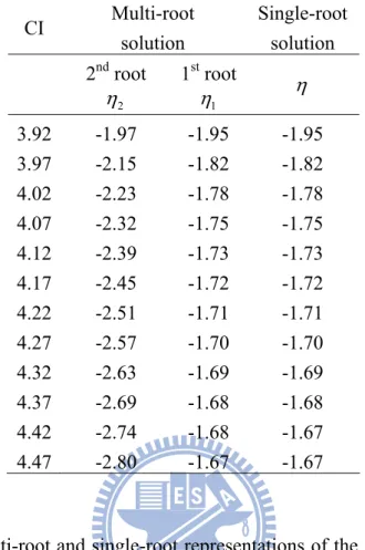
Table 1: the multi-root and single-root solutions of the coverage constraint equation26 Table 2: Some cdf values of CI for single-root representation, multi-root

representation and realistic case by simulation ...27 Table 3: Single-root solutions using different initial conditions ...28 Table 4: The confidence level 1−αof two integration intervals for different sample

sizes ...32 Table 5：Performance of realistic QMI analysis ...44 Table 6: Comparison with different estimators in association with bad initial

searching points (Unit: MSE)...45 Table 7: Comparison with different estimators in association with good initial

searching points (Unit: MSE)...45 Table 8: Computation results for the uncertainty ratio, UR =1.5, with 1,000 trials,

normalized by 2_{( ) /} c

u x n , 4 mixing signals (Unit: Normalized MSE) ...50

Table 9: Table of confusion for the conditions of combined mean and combined standard uncertainty...62

List of Figures

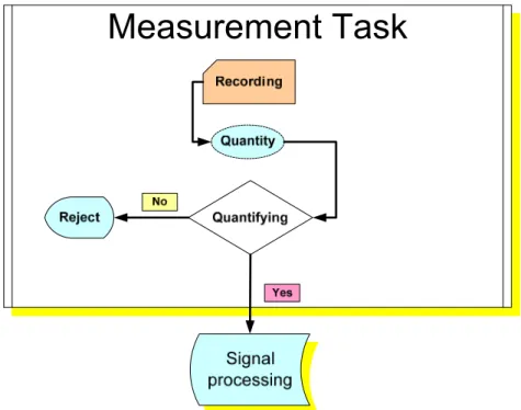
Fig. 1: Measurement is the front stage of signal processing for quantifying data

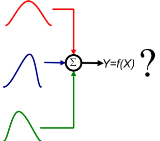
recognized...3 Fig. 2: Un-determined properties of the output pdf resulting from combining different

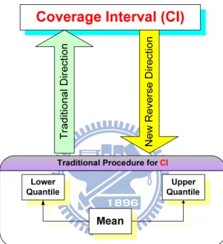
input pdfs. ...4 Fig. 3: This study reverses the traditional direction for CI estimation respect to the

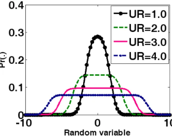
asymptotically symmetry pdf and further extending CI for mean estimation ...5 Fig. 4: An example of the QSAW signal with zero-mean R*N distribution for some

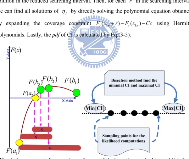
uncertainty ratio (UR)...15 Fig. 5: Profile-conditional pdf by the sampling strategy. k is a constant...21 Fig. 6: A conceptual diagram shows the use of the bisection method to establish the

two endpoints for CI. Here, [a b is an effective interval for root finding and _{1, 1}]

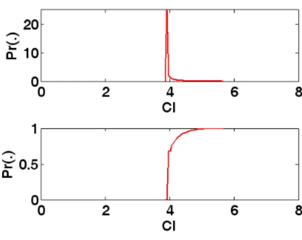
crepresents the center (midpoint) of any new effective interval. ...23 Fig. 7: The pdf (top) and cdf (buttom) of CI for normal random variable with

experiment setting of coverage=0.95 and sample size=15...24

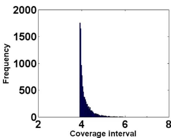
Fig. 8: Histogram of CI generated by simulation using 10,000 trials. The experiment setting is coverage=0.95 and sample size=15. ...25

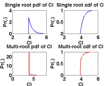
Fig. 9: The multi-root and single-root representations of the pdf and cdf of CI simulated using the standard normal distribution of input with sample size 15 n= , and coverage=0.95. ...27

Fig. 10: The cdfs of CI using single-root representation, multi-root representation, and simulations...28

Fig. 11: Uniform pdf for the random variable s ...30

Fig. 12: The pdf of coverage for some small sample size n...31

Fig. 13: Relation of variables’ interference model ...37

Fig. 14: Relative quantile mapping invariance based on their percentiles. Dash-line represents the original normal pdf and solid-line represents the standard normal pdf. ...40

Fig. 15: Comparison of the conventional sample mean estimator and two coverage-based mean estimators. ...43

Fig. 16: Experimental results for VTNJE using two output patterns of UR=3.7 and 10.4. Left: the distributions of output quantities. Right: MSEs normalized to 2_{( ) /} c u x n ...51

Fig. 17: Performance comparison for six estimators using the first output pattern with UR= 3.7. ...52

Fig. 18: Performance comparison for four estimators using the output quantity of 4-mixture combined quantities with different UR. The average MSE is normalized to 2_{( )} c u x n ...53

Fig. 19: Standard normal pdf combined with its CLT pdf and QSQ pdf for sample size=11. We plot the QSQ of equal variance rectangular pdf [− 3, 3] as the blue solid line. ...59

Fig. 20: MSE of QMLE versus difference=

(

μ_ps−μ

)

for three normal distributions. Note that ξ1:n is calculated using true standard deviation σ ...60

Fig. 21: Conditions A and C. y axis is normalized to 2_{( ) /} c u x n ...63

Fig. 22: Conditions B and D. y axis normalized to 2_{( ) /} c u x n ...63

Fig. 23: Histogram of 50,000 combined quantities for different URs. x-axis is the output of combined quantities and y-axis is the frequency count ...64

Fig. 24: Gain performance for the different URs. The unit is 2_{( ) /} c

u x n ...64

Fig. 25: Good sample mean tested with the convex sets, normalized by 2_{( ) /} c

u x n ,

sample size is 15, 4 combined quantities...65 Fig. 26: Originally left biased of bad sample mean tested with the convex sets, double

y-axes, normalized by 2_{( ) /} c

u x n , sample size is 15, 4 combined quantities...66

Fig. 27: Originally right biased of bad sample mean tested with the convex sets, double y-axes, normalized by 2_{( ) /}

c

u x n , sample size is 15, 4 combined

quantities...67 Fig. 28: Refined Q2MMSE-CLT with the enlarging standard uncertainty, y-axis is

normalized by 2_{( ) /} c

u x n , 4 combined quantities...67

Fig. 29: Nonlinear estimators compared to the sample mean estimator for different uncertainty ratio (UR), y axis is normalized to the combined standard

uncertainty, 2_{( ) /} c

u x n ...69

Fig. 30: The pdfs of QSQ of the MP pair (i.e., normal and rectangular distributions) for the case of μ=0, σ =1, and n=11. Dots on x-axis are expectation values of QSQ. ...73 Fig. 31: The performance of QMLE-QSQ mean estimation for different degree of

deviation of the transform-domain quantile used to the true one. Note that y axis is normalized by 2_{( ) /}

c

u x n . ...75

Fig. 32: The mean estimation performance of QMLE-QSQ using two different quantile-expectation (QE) replacement schemes for two QSAW signals: (a) UR=3.7 and (b) UR=10.4. The y axis is normalized by 2_{( ) /}

c

u x n . Note that the

MSEs of QMLE-QSQ and sample mean are

* * 2 1 10000 2 1 ( ) 10000 2 ( ) ( ) ( ) n i c i i n u x μ μ μ = + − ⋅

∑

and 2 10000 2 1 ( ) 10000 c( ) i n u x = μ μ − ⋅

∑

, respectively...76

Fig. 33: The performance of UBE finding using the proposed QMLE-QSQ mean estimator ...78

Chapter 1: Introduction

1.1 Motivation

The observation of nature which constitutes an experiment will almost inevitably take the form of a measurement. Measurement is represented as the precision type related as whether the experiment is effective, or in the other words, how much is taken about its confidence corresponding to the experiment.

Does the measurement merely have the purpose of standing for a qualitative conclusion? Such a question causes the focus of the meaning of any experiment whenever it is significant not only for someone’s special idea but also lay themselves open to all the frailties of human judgments. That is, confidence report is needed in the formal measurement report. According to the requirement of duplicate verifications for the results of any new approach, the workers expect to convey the experimental results to someone else based on the condition of laboratory or field testing invariantly so that the level of confidence must be also included in the measurement task. Besides, confidence plays the key role to support whether to accept the other’s report so as to avoid performing a duplicate experiment. Thus the center problem for measurement task includes showing the confidence level about the results.

The best qualification of measurement is admitted as a statement of the result of human’s observations with high confidence. Because of this fundamental role of measurement it is necessary to consider in some detail what a measurement practically is. That is, how much confidence does we believe in the observations? Why does the measurement task pay attention to the confidence factor associated with the practical experiment? According to the scientific revolution, we think that the “uncertainty principle” brings the reason for any measurement event, especially in micro-electronics ones. For the reason to overcome the uncertainty representation, the Physics Laboratory of National Institute of Standards and Technology (NIST) conducts the standards and measurement method for electronic, optical and radiation technology for US. and takes the general Type A or Type B expression as the report for measurement task.

NIST keeps the policy based on the approach to expressing uncertainty in measurement recommended by the CIPM1and the evaluation given in the Guide to the Expression of Uncertainty in Measurement (GUM), which was prepared by individuals nominated by the BIPM, IEC, ISO, or OIML. GUM is the most authorized reference on the general application to express measurement uncertainty till 1995. After that time, the Joint Committee for Guides in Metrology (JCGM) collects the above document and releases the new methods and standards for measurement. Thus this study will keep the work to follow the document published by JCGM as the reference. Although JCGM spent a long time for the general expression of uncertainty measurement, there are some occasions not included for practical applications and we focus on those which measure the combined signals on sparse data condition.

1.2 Stating the Function for Coverage Interval

Signal processing is a basic technique to process the sensoring signal and further sends the processed signal to the next stage or outputs it. In addition to choose a proper singal processing technique, we also need some other tools to check the properties of the input signal, such as coverage interval (CI), normal range, and reference interval, in order to determine whether the input signal is quantified to take the utility. CI is the predicative interval including a measured random quantity based on a pre-specifyied proportion of population. It is frequently applied to the cases with normal population assumption where they take the minimal CI to replace all other possible values of CI. The principal function of CI is to state the confidence and uncertainty about the measured quantities. It defines the prediction interval of values where 95% of the population fall into as suggested by JCGM [33]. For instances, we may reject the outlier data from the measured signal if the data are away from the mean value grater than 2 times of the standard deviation. A risk representation can also be applied by the way of CI to make a reject decision on sampling data if its value is out of the CI extent.

CIPM: International Committee for Weights and Measures BIPM: International Bureau of Weights and Measures IEC: International Electrotechnical Commission ISO: International Organization for Standardization OIML: International Organization of Legal Metrology

Fig. 1: Measurement is the front stage of signal processing for quantifying data recognized

Although CI is used as the standard item for the JCGM format of measurement tasks, there still have some shortcomings not being overcomed so far. The most commomly encountered problem is that CI is usually evaluated based on the assumption that the population has a asymptotically symmetric pdf, but we know this is not always appropriate, especially at the occasion of combined signal. The other CI computation method is the non-parametric method which is constructed basing on the percentile evaluated by the expectation of order statistics [1]; that is, we may take the quantile mapping to the corresponding percentile as the desired endpoint. The main difficulty of using CI for combined signal is that we don’t know whether the symmetry property of the output signal is valid when applying the CI computng algorithm. There are still other statistical techniques, such as logarithm transform and Box-Cox transformation, suggested for enhancing the symmetry properties of the analyzed signal and the outliers examining are also necessary.

1.3 Goal and Scope

Combined signal is one of the most popular measured signals for the practical usage and is widely applied to the field test as well as to the industry production. In GUM, a combined signal is represented by an additive model in which the pdf of the output

signal is modeled as the result of a propagation of input pdfs. Some special areas concern the measurement task of combined signals and treat it as an integration of the affecting factors caused from the environment.

∑

?

Fig. 2: Un-determined properties of the output pdf resulting from combining different input pdfs.

In accordance with the report expression of JCGM 101, coverage interval (CI) with its two endpoints, mean value and standard uncertainty are the three members of its main concern. They are also the main concern of this study. Due to the fact that the output of combined signal is random, we think the best description for CI representation is to formulate its pdf . Issues addressed are briefing as follows. First, we are interested in the formulation to unify the CI representations for skew and non-skew pdfs. Conventionally, different approaches are employed for these two types of pdfs to calculate their respective CI. Besides, we are also interested in the truncated probability density function normalized to its coverage. The non-skew, asymptotically symmetric pdf draws our special attention because it is the typical output pdf shape of combined signals. Moreover, the usual evaluation of asymptotically symmetric CI involves the interval composing of an upper quantile (half coverage) and a lower quantile (half coverage) with respect to the mean value. A robust CI estimation needs accurate quantile and mean formulations. This is the rule followed in the past studies so is the current study. There are a few exceptions to the rule. One is that we can consider giving a robust CI before the mean estimation, and this may leads to a good performance for mean estimation. A study will hence be conducted to try to use the traditional coverage interval to assist in the mean estimation. The issue is that if we are giving a more accurate coverage interval, can we make some progress on improving the mean estimation? Besides, we will

introduce three new approaches of mean estimation and compare them with the classical sample mean estimator. They include a quantile-based mean estimator using the coverage interval, a nonlinear mean estimator and a robust statistical one using the minimax principle. Lastly, we will shape the proposed quantile-based mean estimator to a quasi-symmetric quantile-based one and use it in an application to find the upper bound of the maximum eigenvalue (UBE), to examine the usage of the robust JCGM expression in measurement.

Fig. 3: This study reverses the traditional direction for CI estimation respect to the asymptotically symmetry pdf and further extending CI for mean estimation

Chapter 2: Paper Review

We review some literatures related to the three main topics discussed in the dissertation. They include coverage interval which is a member of JCGM expression, mean estimator, and finding UBE, which is an application of mean estimation. The sampling size requirement will be especially concerned in the following discussions.

2.1 Coverage Interval

Coverage interval (CI) is originally regarded as a parameter to represent the uncertainty of measurement. Fotowicz [2] proposed an analytic method to calculate CI from the distribution of the output of combined quantities, formed by taking the convolutions of the pdfs of its constituents which were assumed to be rectangular mixing with one of Student’s t-, triangular, or normal distributions. It made some progress in the realization of CI without using complex numerical computations. Nadarajah [3] continued to extend the algorithm and applied it to a wide range of usage with higher degree of freedom. In those studies, CI was always used as a confidence measurement in the sampling plan.

CI is affected by coverage constraint realistically. If we turn to a different viewpoint relating to the coverage problem, the “statistical CI” is also a good tool to describe the uncertainty. Wilks [4] proposed a statistical CI, defined by

1 2

{ [( , )]_x } 1

Pr p T T ≥β ≥ − , (2-1) α

to describe the probability that a random variable x includes a β-content proportion of the population or more in the interval [ , ]T T is greater than the threshold _{1 2} 1−α . The statistical CI has been proved to represent a certain confidence level [45]. In those past studies, the confidence level was usually obtained by the Monte Carlo simulations [ 5 , 6 ].There were some previous studies concerning the issue of randomness of coverage. The early topic was called “the random division of an interval”, which means the range may be cut as many small sub-ranges which can be added to calculate the coverage [7,8].

The representation of CI can be categorized into two classes: parametric and non-parametric CI. Lin et al. [9] suggested using a non-parametric formulation to calculate CI when the population pdf is unknown. Chen [47] suggested that, while adopting the parametric CI approach, it had better take the minimum of all possible values of CI for computational simplification. In the past, CI was mainly applied to the cases of resource constrained for the original population. For instances, a clinical chemistry experiment first applies tests to healthy people to create a CI, and then takes the same test to a patient and collects the outputs. If the outputs are out of the CI, it implies that the patient has got a disease. In medical engineering, to collect large samples containing all the records of patients is a time-consuming task so that we should sometimes take a sampling plan of small sample size. Thus data sparseness is inevitable in this kind of application because the process of collecting data is time-consuming and expensive.

The use of CI is popular for the chemical substances in biological fluid for reference population [10], and for some other related fields of measurement. The International Federation of Clinical Chemistry and Laboratory Medicine (IFCC) [11] has published a series of recommendations for the advanced utilizations of CI. IFCC defined the percentile between 0.025~0.975 as the standard CI of 95% reference interval, and suggested that the best population (reference values) size had better be greater than 120 so that a high confidence reliability can be guaranteed. IFCC made more rules and standards for the reference interval estimation and computation, but without further addressing the issue of the influence of sample size. This study discusses the CI problem concerning the size of sample data and deals with how to control the categories of influences if the sample size is far less than 120. We will take a new viewpoint to analyze the effect of sample size on CI. Actually, it is not necessary to formulate CI from the viewpoint of the aggregation method. If we evaluate the two endpoints of CI separately, we may consider estimating CI with the quantiles based on order statistics. The quantile-based estimator [12] was recently proposed by Heathcote et al. It performed very well for the response time estimation and showed high efficiency to the parameter estimation for some distributions.

2.2 Mean Estimation

The second topic we are interested is the mean estimation of population. We will try to use CI in the mean estimation basing on the asymptotically symmetric pdf assumption. In this case, mean is the midpoint of the two endpoints of CI and we truly believe that a more accurate estimation for CI will lead to a more accurate estimation for mean value.

In parameter estimation of using normally-distributed sparse data, there are two popular methods: the best linear unbiased estimation (BLUE) method and the maximum likelihood estimation (MLE) method. Balarkrishnan and Cohen [13], Lloyd [14], and Teichroew [15] proposed the BLUE method for parameter estimation of normal random variables by using order statistics. BLUE is a weighted least-square algorithm basing on the Gauss-Markov least-square theorem. It was popularly used for sparse data analysis. It is known that BLUE is unbiased and more efficient if it takes the censoring sampling scheme. We briefly discuss BLUE as follows.

Let x be a normal random variable with pdf _{( ) ( ,} 2_). x

f x =N uσ Assume that there are n independent observed samples x₁, ,_L x_n of x. Let x_1:n, ,_L x_{n n:} be the ranked samples of x₁, ,_L x_n in increasing order. The BLUE estimator is formulated as the sum of products of the observed data and properly-chosen coefficients. By performing the standard normal transformation, =(ξ_i x u_i− ) /σ, to the observed data and sorting them in increasing order, we have

1 [ , , ]T n n X = x _Lx 1 [ , , ]T n ξ = ξ _L ξ

{ }

i n: i n: E ξ =ρ : : , : { _{i n}, _{j n}} _{i j n} Cov ξ ξ =β

{ }

{ }

i n:n i n: E x u E X u σξ σξ = + = Ι + (2-2)

[

]

1 I_{n = L}1, ,1T_n×

2

B=σ I (2-3)

for 1≤i j n, ≤ and i< , where Ij _n is an n-dimensional all-1 vector. Consider the

generalized variance:

(

_I

)

T 1

(

_I

)

n n n n

X ₋u ₋σξ B− X ₋u ₋σξ _(2-4)

Minimizing it with respect to u and σ, we obtain.

1 1 1 1 1 1 I I I I I T T T n n n n n T T T n n u B B B X u B B B X σ ξ ξ σξ ξ ξ − − − − − − + = + = (2-5)

The solution of Eq.(2-5) is

1 1 1 1 * 1: : 1 1 1 2 1 I I ( )(I I ) ( I ) T T T T n T n n n n i i n T T T i n n n B B B B u X X x B B B ξ ξ ξ ξ _{ξ α} ξ ξ ξ − − − − − − − = ⎧ − ⎫ =_{⎨ ⎬} = − Δ = − ⎩ ⎭

∑

(2-6) 1 1 1 1 * 2: : 1 1 1 2 1 I I I I I ( )(I I ) ( I ) T T T T n T n n n n n n n i i n T T T i n n n B B B B X X x B B B ξ ξ σ α ξ ξ ξ − − − − − − − = − = = Δ = −

∑

(2-7)

where _{u and} * _σ* _{are the estimated parameters, and} 1:i

α and α_2:i are weighting coefficients. These coefficients have been tabulated by Sarhan and Greenberg [16,17] with entries in the 1956 tables being given for sample size up to 10 and in 1962 up to 20.

Generally speaking, BLUE performs well in small sample size. But it needs a table to look up, and this is a shortcoming. The other technique used is the MLE method which is often applied to the truncated normal distribution in sparse data condition. Cohen [54] derived the singly truncated and doubly truncated maximum likelihood estimators and found that they outperformed BLUE when the sample size was greater than 20. Cohen recognized the sparse data problem as a truncated normal pdf and defined its likelihood by

2 1: 1: 2 1 1: 1: ( ) ( ) ( ) exp( ) 2 2 ( ( ) ( )) n n n n i i x n x n UnitStep x x UnitStep x x r x u L F x r F x σ πσ = ⎛ _{− − − −} ⎞ ₋ =_{⎜⎜ ⎟⎟} − + − ⎝ ⎠

∑

(2-8)

If we take the transformations of ξ_1:n =(x_1:n−u) /σ and ξ_{n n:} =(x_{n n:} −u) /σ and differentiate the resulting log-likelihood function with respect to u and σ , we obtain the following two equations.

1: : 2 1 : 1: 1: 1: : : 2 2 1 : 1: ( ( ) ( )) 1 ( ) ( ( ) ( )) ( ( ) ( ) ( )) 1 1 ( ) ( ( ) ( )) n n x n n i i n n n n n n n n n n i i n n n n x u x u n ξ ξ ξ ξ ξ ξ ξ φ ξ φ ξ σ ξ ξ σ ξ φ ξ ξ φ ξ σ ξ ξ = = − = − Φ − Φ ⎧ − ⎫ ⎪ ₊ ⎪_{= −} ⎨ _{Φ − Φ} ⎬ ⎪ ⎪ ⎩ ⎭

∑

∑

(2-9)

where φ and Φ are the standard normal pdf and cdf, respectively. By defining two new random variables

1: 1: 1: ( ) ( ) ( ) n L n rs n ξ ξ ξ φ ξ ξ ξ Θ = Φ + − Φ and 1: 1: 1: ( ) ( ) ( ) n s R n s n r r ξ ξ ξ φ ξ ξ ξ + Θ = Φ + − Φ ,

we obtain the following two equations

1: 1: 1 1: : : 1: ( , ) n L R n n n n n n n x x H r ξ ξ ξ ξ ξ − Θ − Θ − = = − (2-10)

(

)

2 2 1: 2 2 1: : 2 2 : 1: 1 ( ) ( , ) n L R L R n n n n n n S H r ξ ξ ξ ξ ξ ξ + Θ − Θ − Θ − Θ ⇒ = − (2-11)

2.3 The Method Suggested by Cohen

Cohen proposed a method to estimate mean and variance of normally distributed random variable. Let L

L x u ξ σ − = and R R x u ξ σ −

= , where x and _L x are the left _R

and right truncation points, respectively. The standard deviation can be estimated by:

R L R L x x σ ξ ξ − = − .

The method first models all data samples by a truncated normal distribution shown below: 1: 1: 1: 1: ( ) ( ) ( ) ( ) ( ) ( ) x n n T x n x n f x UnitStep x x UnitStep x x r f x F x r F x − − − − ⇒ + − (2-12)

where the left truncation point x is replaced by the minimum order random variable _L

1:n

likelihood function by 1: 1: 1 ( ; , , _n, ) n ( ( ; , ,_{T i n}, )) i L x u σ x r f x u σ x r = =

∏

(2-13) By taking { ( ; , ,L x u x r_1:n, )} 0 u σ ∂ ₌ ∂ , it obtains 1: 1: 2 1 1: 1: ( ( ) ( )) 1 ( ) ( ( ) ( )) n x n x n i i x n x n n f x f x r x u F x r F x σ σ = − + = − + −

∑

(2-14)

It then takes the standard normal transformations for the two endpoints of ranked samples, x and _1:n x , to obtain _{n n:}

1: 1:n n x u ξ σ − = and : : n n n n x u ξ σ − = .

The corresponding CI in the transform domain is r_s =ξ_{n n:} −ξ_1:n. It is noted that the cdf,

( )

ξ ξ

Φ , of the transformed random variable is related to the cdf, ( )F x , of the _x

original random variable by F x_x( _1:n)= Φ_ξ(ξ_1:n) and F x_x( _{n n:} )= Φ_ξ(ξ_{n n:} ). By denoting

1: 1: 1: ( ) ( ) ( ) n L n rs n ξ ξ ξ φ ξ ξ ξ Θ = Φ + − Φ and 1: 1: 1: ( ) ( ) ( ) n s R n s n r r ξ ξ ξ φ ξ ξ ξ + Θ = Φ + − Φ , it has ( _{L R}) x u− =σ Θ − Θ (2-15) By taking { ( ; , ,L x u σ x r_1:n, )} 0 σ ∂ = ∂ , it obtains 2 1: 1: 1: 1: 3 1 1: 1: ( ( ) ( ) ( )) 1 ( ) 0 ( ( ) ( )) n n x n n x n i i x n x n n x f x x r f x r n x u F x r F x σ σ σ = − − + + − + − = + −

∑

(2-16)

Eq.(2-16) can be further simplified and expressed by

{

}

1: 1: : : 2 2 1 : 1: 2 2 2 2 2 1 2 1 1 ( ( ) ( ) ( )) 1 1 ( ) ( ( ) ( )) 1 1 1 ( ) ( ) ( ) n n n n n n n i i n n n n n L R i i i x u n x x x u S x u n n ξ ξ ξ ξ ξ φ ξ ξ φ ξ σ ξ ξ σ ξ ξ = = = ⎧ − ⎫ ⎪ ₊ ⎪_{= −} ⎨ _{Φ − Φ} ⎬ ⎪ ⎪ ⎩ ⎭ Θ − Θ + = − + − = + −

∑

∑

∑

(2-17)

where x and _{S are mean and variance of the data samples. If} 2 _{σ is known, the}

If σ is unknown, Cohen suggested to solve the following two equations: 1: 1: 1 1: : : 1: ( , ) n L R n n n n n n n x x H r ξ ξ ξ ξ ξ − Θ − Θ − = = − (2-18)

(

)

2 2 1: : 2 1: : 2 2 : 1: 1 ( ) ( , ) n L n n R L R n n n n n n S H r ξ ξ ξ ξ ξ ξ + Θ − Θ − Θ − Θ ⇒ = − (2-19)

where w r= , v1= −x x1:n, and r is the range of the data samples. Eqs.(2-18) and

(2-19) can be solved by the Newton and Raphson method. But, it is time-consuming unless good initial values are provided. Alternatively, Cohen [18] proposed the following iterative procedure to solve them:

(

)

( 1) 1: ( ) ( ) : ( 1) 1: 1: 1 i n i i n n L R i n n x x r x x r ξ ξ + + − ⎧ ⎫ − _{⎨ ⎬}+ Θ − Θ ⎩ ⎭ = − ⎛ ₋ ⎞ ⎜ ⎟ ⎝ ⎠ (2-20)

(

)

( 1) : 1: i n n A Br x x n r ξ + _{= + − − (2-21)}

(

( )i ( )i

)

L R A= Θ − Θ 2 2 2 2 4 2 S C C r B A S + + = + ( ) 1:n i R x x C A r − = + Θ

S: variance of the test sequence

r : range of the test sequence i : iteration index

2.4 Sample Mean Estimator

In the past, sample mean is widely used in the mean value estimation for any signal no matter what its original pdf is. The main reason of using sample mean is that it is not only a uniformly minimum variance unbiased estimator (UMVUE) but also a random variable of the central limit theorem (CLT). In this study, we will propose a new mean estimator basing on the proposed CI representation and compare its performance with the traditional sample mean estimator [19]. Our study will specially focus on the mean value estimation problem for the output of combined quantities in

the sparse data condition. Bowen [20] has pointed out that CLT may be explained as the sum of independent variables with the characteristic function formed by the product of the component characteristic functions. If we can ignore the unbiased requirement, there exist some biased estimators that outperform sample mean. Stearls [21] and Gleser [22] discussed a new approach to giving coefficients of variation of sample mean. Ashok et al. [23] further proposed a realistic method to adjust the coefficients of variation of sample mean to improve its performance.

Up till now, if we want to predict the mean value of combined quantities accurately, the only way is to take the sample mean on heavy observations. In practical applications of measurement, the basic volume required for one digit accuracy is ₁₀ 6

observations for 95% coverage interval [24]. If, there are not enough samples to support this rule, a medium- or small-size sampling plans should be taken. Besides, the good property of UMVUE for sample mean may be ineffective for the case of combined quantities which is of quasi-normal distribution. This is because the property of UMVUE is derived from the maximum likelihood estimation (MLE) on the basis of the normal pdf assumption.

In this dissertation, a new method of mean value estimation, referred to as the quantile-based maximum likelihood estimator (QMLE), is proposed. The classical application of quantiles is the general usage of empirical quantiles. Koenker and Bassett [25] extended the empirical quantiles to the regression quantiles, which is specially useful for predicting the bounding information. Gilchrist [26] collected many studies about the estimation, validation, and statistical regression with quantile models. In the single quantile application, Giorgi and Narduzzi [27] gave the quantile estimation for the self-similar process.

In the proposed QMLE, the quantiles are determined by the maximum percentage of population, i.e. coverage, so that it is composed of a couple of quasi-symmetric quantiles (QSQ). According to the past studies, the coverage-constrained quantiles will obey the properties of symmetric quantiles whose variances asymptotically approach to the Cramer-Rao lower bound [ 28]. The symmetric quantiles were described with strict definition given in [28]. But we treat them in a more flexible way as the ranked variables of the first ordered sample x and the last ordered sample _1:n

: n n

x . Hence the QSQ we considered are both empirical and quasi-symmetric quantiles.

Lo and Chen [29,30] also derived good quantile-based estimators for the sparse data condition. In this study, we plan to derive the QMLE basing on the order statistics and expect that it can support not only the concept of empirical quantiles but also the quasi-symmetric quantiles. Otherwise, we would still need a quantile function defined below to link quantiles and MLE

( ) Pr( _p)

Q p ≡ X ≤x = (2-22) p

Here, the value x is called the p-quantile of population. _p

2.5 Quantizing the Combined Signal

Generally speaking, the measured quantities are affected by unknown noise so that they are always expressed in random representation. In the past studies, Fotowicz [2] suggested using “uncertainty ratio” to represent the combined signal comprising at least one input quantity with rectangular distribution. Suppose z , i 1 i N≤ ≤ , are

independent signals and c , _i 1 i N≤ ≤ , are corresponding weighting coefficients, then the linearly combined output x can be expressed by:

1 1 2 2 N N

x c z= +c z + +_L c z . (2-23)

The pdf of x is an R*N distribution which is the convolution of a rectangular distribution and a normal distribution, and can be expressed by:

( )

2 3( ) 2 3( ) 1 ( ) 2 6 t x UR RN _{x UR} c f x e dt K π UR − + − =

_∫

, (2-24) where 2 2 [ ( )] ( ) [ ( )] i c i Max u x UR u x Max u x = − ; (2-25) 2 2 2 1 ( ) N ( ) c i i i u x cσ z =

=

∑

is the approximate variance of the combined signal; ( )σ z_i is the standard deviation of z ; _i K is a normalization constant; and ( )_c u x is the _i

standard deviation of the i-th input random variable which is subject to the rectangular distribution. The endpoint of p-quantile for the R*N distribution can be

expressed by 2 1 ( ) ( ( )) N p RN i i N t v U k u y k μ = = +

∑

, (2-26)

where μ is the population mean, 3₂ (1 ( ) 2 ( )(1 )) ( ) 1 RN k UR UR c UR = + − − + is a

coverage factor, c is a coverage, t v is a quantile of Student’s t-distribution, ( ) k _N

is the corresponding quantile of coverage factor, e.g. k =1.96 for _N c=95%, and N is the number of input quantities. If the distribution of the i-th input random variable coincides to be a normal, rectangular, Student’s t-, or triangular distribution, then

( ) / _N 1

t v k = .

Fig. 4 displays the R*N distribution for UR = 1, 2, 3, and 4. According to Fig. 4, we describe the measured signal of combining quantities by additive mixture model as quasi-normal signals with asymptotic window-shape distribution (QSAW). A common property of QSAW signals is that they are usually distributed flatter than the normal pdf in the central part and then sharply decaying to zero at both ends. As shown in Fig. 4, the pdf of a QSAW signal looks like a normal distribution for small UR and a rectangular distribution for large UR.

Fig. 4: An example of the QSAW signal with zero-mean R*N distribution for some uncertainty ratio (UR)

2.6 The Issue of Application to the Finding of UBE

In this study, we will consider the use of robust mean estimation in signal detection. Generally, the energy-based signal activity detection approach is robust to noise and may cost down the non-coherent detection within a communication receiver. Zeng et al. [31] showed the benefits of using the maximum eigenvalue as a result of energy representation on large sample size. Recently, compressive sampling (CS) [32] is an emerging research topic aiming at restoring a signal in an undersampled condition using special vector bases with prior knowledge of the signal. In addition to CS, eigen-analysis is also a popular technique to consider spanning a signal with sparse eigenvectors in which the prior knowledge of needing signal to be normally distributed is released. We will not only consider the combination of energy detection and sparse data sampling, but also fuse the demand of practical signal processing. For instance, measuring signal in a time-varying environment usually results in representing the measured signal as the output of combining quantities by an additive mixture model, as suggested and outlined in the manual published by JCGM [33]. Moreover, the combined quantities are usually resulted from the propagations of multi-source signals with different pdfs so that the representation for the pdf of the output random variable is not tractable.

Unexpectedly, the pdf of the maximum eigenvalue is too complex and inconvenient for computation [34] so that Ma and Zarowski [35] have tried to use the upper bound of the maximum eigenvalue, i.e., Dembo’s bound, for an efficient signal representation. In the study, we are interested in using more accurate mean estimation to improve the finding of upper bound of eigenvalues (UBE) from sparse observed samples.

Since the environmental noise is usually time-varying or color, the traditional white-noise assumption is not realistic so that the mean value of noise can not always be regarded as zero. Hence this study proposes a new algorithm to evaluate the mean value in terms of noise combined with signal.

Let x , _{i n:} 1 i n≤ ≤ , represent the ranked random samples generated from the output of

Eq.(2-23). In this study, we plan to estimate the mean value of a QSAW signal by a new quantile-based maximum likelihood estimator (QMLE) using only the

quasi-symmetric quantiles (QSQ), i.e., the minimum sample, x , and the maximum _1:n

sample, x . We will compare the performances of the QMLE and sample mean on _{n n:}

mean estimation as well as on UBE finding.

There are two parts in our task: one is the QMLE mean estimation aiming at reducing the uncertainty of the estimated correlation matrix and another is the improved upper bound of eigenvalues finding. Conventionally, the mean value of a signal is estimated by sample mean which is UMVUE derived basing on the assumption of normally distributed observations. Although sample mean is a good mean estimator, there still exist some biased estimators that outperform it [23]. In mean estimation for quasi-normal signals, the non-parametric order statistics method was applied to overcome the mismatch between normal and quasi-normal data. In the study, we are interested in the special case of quantile application to mean estimation using the QSQ. The QSQ are determined by the maximum percentage of the observed samples covering the original population, i.e., the coverage which is the cumulative probability calculated between the two endpoints of range. There are good evidences to show that the symmetric property of QSQ is more efficient if they occupy either a very large or very small percentage of the population [36]. Lastly, the task of UBE finding is attractive because the maximum eigenvalue is an important cue of signal activity detection for fading channels with unknown dispersion [31] in multiple-input multiple-output (MIMO) systems [37]. Taparugssanagorn and Ylitalo [38] further indicated the upper bound of MIMO channel capacity being affected by the distribution of the maximum eigenvalue, which was evaluated by the covariance of short-term phase noise. Zhang and Ovaska [39] extended the eigenanalysis to singular value decomposition based on signal-to-noise ratio for the analog-to-digital converter, but their method is not realistic for the cyclostationary detection in spectrum reuse application. Wu et al. [40] proved that the well-trained eigenvector feature of vehicle sound signature was capable of vehicle recognition. UBE acts as the maximum eigenvalue owing to the fact that this representation has been well discussed for the case of deterministic covariance matrix with Hermitian, symmetric positive-definite, or Toeplitz property, Park and Lee [41] improved it by using the technique of series expansion. They proposed the following equations to find a better upper bound of maximum eigenvalue than the classical Dembo’s bound:

(m1) (m1) m m H R b R b a − × − × ⎡ ⎤ = ⎢ ⎥ ⎣ ⎦ (2-27)

(

1 (

)

1) ( 1) ( 1) ( 1) 1 1 0 1 1 ( ) H i r m m m H i r i m m r i m b R b g ε a ε r b R b η ε ε η ε − − × − − × − + + = − ⋅ = − + + − ⋅

∑

, (2-28)

where R_{m m×} is the correlation matrix of the input signal, r > 0 is the order index, ε is an eigenvalue, η_m−1 is the maximal eigenvalue of R_{(m− × −1) (m1)} , b is an (m-1)-dimensional vector, and a is a scalar. Up till now, there are seldom studies devoting to the uncertainty analysis for the estimation of correlation matrix on sparse data condition. This study proposes the refreshing change-solution against the issue. It avoids the well-known heavy resampling and computation of the bootstrapping method [42] for small sample size. The main uncertainties of additive model result from the propagation of each source signal. In the reasoning for uncertainty of propagation, Denguir-Rekik et al.[43] fused the multiple marginal effects based on the multi-criteria for aggregated decision making. Ferrero and Salicone [ 44 ] addressed the issue of utilizing the random-fuzzy variable to fit the propagation of distribution.

Chapter 3: The Probability Density Function of Coverage

Interval

3.1 Introduction

Coverage interval (CI) is an interval with two confidence extremes that covers a specified portion of the population. It has been intensively studied in recent years in biology, quality control, medical engineering, and some other research areas. CI is called reference interval in clinical chemistry [45] and is constructed based on the reference values belonging to the population. Motivated by the needs of processing data on small sample size condition for some newly developing areas, such as data mining for knowledge exploration and data representation for pattern recognition, this study deals with the problem of expressing CI under sparse data condition. The issue of applying CI representation to parameter estimation to against the large uncertainty caused by sparse data will also be addressed.

The International Organization for Standardization has issued a document, ISO GUM Suppl. 1: Guide to the expression of uncertainty in measurement supplement 1 [24], to recommend applying CI as an expression of uncertainty measure to meet the recent trend of treating CI in a probabilistic way. The GUM method of evaluating and expressing uncertainty has been adopted widely by the industry. It can also be found from the manuals published by the Joint Committee for Guides in Metrology (JCGM) [46] that the probability assigned to the input quantity is important. But, a weakness of the probability assignment suggested by JCGM lies in the use of deterministic CI. A general way to represent CI, referred to as “parametric CI” [47], is based on defining a symmetric pdf for the input random variable. Alternatively, non-parametric CI representation is based on the empirical distribution of input data. It is usually applied to the case of skew distribution or to the case when the pdf is unknown. But, the dichotomy for CI representation is imperfect if a quasi-symmetric pdf is encountered. To solve the problem, a unified expression for the uncertainty representation of CI is proposed in this study.

Why should we need CI? It is well known that the information of an event can be represented as the logarithm of the reciprocal of its occurrence probability. It is the commonly used uncertainty measure of an individual event. Entropy is defined, from a macro view, as the expectation of the total information. Although both entropy and CI are macro view of sample data, entropy does not act like CI to provide a clear bounding message. This is analogous to the case of calculating the confidence interval of a parameter estimate. Confidence interval can show explicit bounding information for the estimated parameter.

The chapter is organized as follows. In Section 3.2, a new representation of CI is proposed. It adopts a new method to derive the pdf of CI. The effectiveness of the proposed CI representation is evaluated by simulations discussed in Section 3.3. A realization of the statistical CI is presented in Section 3.4. Section 3.5 describes an extension of the statistical CI to the variably truncated normal joint (VTNJ) pdf.

3.2

A New Method to Formulate the

pdf

of CI

In this study, we regard CI as a random variable representing the bounded range to meet the coverage constraint. We now derive the pdf of CI. According to the work based on the general pdf of order statistics [48], the pdf of range can be expressed in a non-parametric form by 1: | , | 1: 1: 2 1: 1: 1: 1: 1: ( ) ( , ) ( 1) ( ) ( )( ( ) ( )) n r n r x n n n n x n x n x n x n n f r f r x dx n n f x f x r F x r F x dx ∞ −∞ ∞ ₋ −∞ = = ⋅ − + + −

∫

∫

, (3-1)

where ( )f x_x and F x_x( ) denote the pdf and cdf of random variable x, respectively;

1:n

x is the minimum order of ranked samples; r is the range of samples; and n is the sample size. It is known that the range pdf shown in Eq.(3-1) is accurate for all realistic cases.

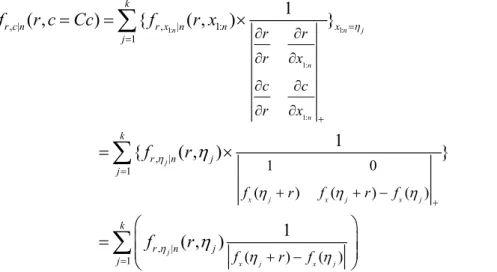
We then perform the variable transformation to change the variable x_1:n to c with range r being preserved, where c F x= _x( _1:n+ −r) F x_x( _1:n) is the coverage. Suppose that there are k roots η_j, 1≤ ≤ , of j k x_1:n satisfying the coverage constraint

equation F x_x( _1:n+ −r) F x_x( _1:n)=Cc with a given constant coverage Cc. The joint distribution of r and c can then be expressed by

1: 1: 1: 1: , | , | 1: 1 , | 1 , | 1 0 ( ) ( ) ( ) ( ) ( ) 1 ( , ) { ( , ) } 1 { ( , ) } 1 ( , ) n n x j x j x j x j x j n n j j j k r c n r x n n x j k r n j j r n j r r r x c c r x f r f r f f r f f r c Cc f r x f r f r η η η η η η η η η η = = + = + ∂ ∂ ∂ ∂ ∂ ∂ ∂ ∂ + + − + − = = × = × ⎛ ⎞ = _⎜⎜ ⎝ ⎠

∑

∑

1 k j= ⎟⎟

∑

(3-2)

It is worthwhile to note that the above expression for the joint pdf of r and c does not explicitly include the coverage variable c. Instead, c is implicitly included through the roots of the coverage constraint F_x(η+ −r) F_x( )η =Cc for each given sample of

c Cc= .

We now take a new viewpoint, which is different from the traditional Bayes’ theorem, to derive the conditional pdf f_{r c n| ,} ( )r . The general form of the Bayes’ conditional pdf

usually maps to a surface while our approach only needs some profiles in the same surface. The concept is shown in Fig. 5 and is realized by

, | | , , | ( , ) ( ) ( , ) r c Cc n r c Cc n r c Cc n dr f r c Cc f r f r c Cc = = = = = =

∫

. (3-3)

A problem encountered in the implementation of Eq.(3-3) is how to expand the transcendental function F xx( 1:n+ −r) F xx( 1:n)=Cc in order to find its roots.

Generally, this can be accomplished by using the Fourier series expansion. But, due to the fact that Hermite polynomials can best fit the curve of normal distribution, we apply Hermite polynomial expansion to F x_x( ) in order to efficiently find the solutions of F xx( 1:n+ −r) F xx( 1:n)=Cc. Eq.(3-2) is then expressed by

{

}

2 , | 1 ( 1) ( ) ( ) ( ) ( ) ( , ) ( ) ( ) n k x j x j x j x j r c Cc n j _{x j x j} n n f f r F r F f r c Cc f r f η η η η η η − = = ⎛ _{− + + −} ⎞ ⎜ ⎟ = = ⎜ + − ⎟ ⎝ ⎠

∑

, (3-4)

where η_j∈ and (R f_x η_j + −r) f_x( ) 0η_j ≠ for 1 j k≤ ≤ . The constraint that η_j

must be real is to obey the output rule of Jacobian determinant.

Some modifications are still needed in practical consideration. The basic idea is to neglect some roots of F_x(η+ −r) F_x( )η =Cc which have very low occurrence probabilities. This is realized by setting two bounds for those roots. This is motivated by the general rule of excluding outliers via considering only data in the interval [μ−4 ,σ μ+4 ]σ where μ and σ are the mean and standard deviation of the population. Normalization of Eq.(3-4) is also needed in order to make it obey the basic requirement for probability. The pdf of CI can then be expressed by

{

}

2 | , 1 ( 1) ( ) ( ) ( ) ( ) ₁ ( ) ( , ) ( ) ( ) n k x j x j x j x j r c Cc n j x j x j n n f f r F r F f r Z Cc n f r f η η η η η η − ′ = = ⎛ _{− + + −} ⎞ ⎜ ⎟ = ⋅ ⎜ + − ⎟ ⎝ ⎠

∑

, (3-5)

where (Z Cc n, ) is a normalization factor shown below

{

}

2 1 ( 1) ( ) ( ) ( ) ( ) ( , ) ( ) ( ) n k x j x j x j x j j dr x j x j n n f f r F r F Z Cc n f r f η η η η η η − ′ = ⎧ ⎡ _{− + + −} ⎤⎫ ⎪ _{⎢ ⎥}⎪ = ⎨ _{⎢ ⎥}⎬ + − ⎪ _{⎣ ⎦}⎪ ⎩

∑

⎭

∫

; , 1 , j j k

η ≤ ≤ ′ are the roots of F x_x( _1:n+ −r) F x_x( _1:n)=Cc that satisfy

4 _j 4

μ− σ η≤ ≤ +μ σ . If k′>1, a root-finding procedure is applied to the Hermite polynomial expanded version of F x_x( _1:n+ −r) F x_x( _1:n)=Cc for finding all roots in the interval, [μ−4 ,σ μ+4 ]σ .