揮發性有機物在未飽和土壤中自然揮發之研究

國 立 交 通 大 學

環 境 工 程 研 究 所

碩 士 論 文

揮發性有機物在未飽和土壤中自然揮發之研究

A Study on Natural Evaporation of VOC in Unsaturated

Soils

研究生：俞仲豪

指導教授：葉弘德 教授

揮發性有機物在未飽和土壤中自然揮發之研究

A Study on Natural Evaporation of VOC in Unsaturated

Soils

研究生：俞仲豪 Student：Jung-Hau Yu

指導教授：葉弘德 Advisor：Hund-Der Yeh

國立交通大學

環境工程研究所

碩士論文

Submitted to Institute of Environmental Engineering College of Engineering

National Chiao Tung University in Partial Fulfillment of the Requirements

for the Degree of Master of Science in Environmental Engineering

September 2010 Hsinchu, Taiwan

揮發性有機物在未飽和土壤中自然揮發之研究

研究生：俞仲豪 指導教授：葉弘德

國立交通大學環境工程研究所

摘 要

地面儲存槽的洩漏，是土壤污染主要的污染源之一，發生滲漏後，部分揮發性有機 物(volatile organic compound, VOC)會以非水相液體(NAPL)殘存在土壤中，若經過一 段時間，氣相、液相、及吸附相的 VOC 會處於平衡狀態。若要整治受污染的土層，需先 移除滲漏的儲存槽，隨後 VOC 將會在自然環境下逸散至大氣中，此自然揮發的過程，值 得研究。VOC 存在土壤中，可分為純 VOC 和以多種化合物組成的複合 VOC 兩類，常見的 汽油儲存槽滲漏污染問題，則以複合 VOC 污染居多。在本文中，我們發展了一個數值模 式，描述複合 VOC 殘存相的揮發鋒面移動及地表下莫耳分率的空間分布，在模式中，考 慮於揮發鋒面及其上下三個區域，透過有限差分法及可移動格網，近似求解莫耳分率的 分佈。此外，考慮單一 VOC 污染的問題，將複合 VOC 模式簡化為單 VOC 模式，利用 Boltzmann＇s transformation，求得單 VOC 模式的解析解。本文考慮六個污染案例， 包括有無殘存相解之濃度分佈，以及不同土壤孔隙率、污染物、初始莫耳分率對揮發鋒 面和莫耳分率分布之影響。藉由計算 VOC 揮發鋒面的位置和移動速度，本研究發展的模 式，或可用來分析或評估受 VOC 污染的現地問題。

A Study on Natural Evaporation of VOC in Unsaturated Soils

Student：Jung-Hau Yu Advisor：Hund-Der Yeh

Institute of Environmental Engineering

National Chiao Tung University

Abstract

Leak of underground storage tank is one of major sources for the spill of volatile organic

compound (VOC) entering unsaturated soil. Once leak occurs, some VOCs may present in

soil as residual non-aqueous phase liquid (NAPL) phase. The gas, liquid, and absorbed

phases of VOC may reach equilibrium after a period of time in the soil. To clean up the

contaminated soil, the tank must be removed and the VOC can then evaporate to the

atmosphere. It is of interest to investigate the natural evaporation of NAPL. There are two

types of VOC contamination in soil. One is multi-component VOC while the other is

single-component VOC. Multi-component VOC, composed of several VOC components, is

often found in petroleum leaking problems. This study develops a two-component model

describing the mole fraction distributions of VOCs and migration of evaporation front of the

VOC in NAPL phase in a homogeneous soil system. The model considers three regions

moving grid approach. The model is also simplified to a single-component model which

deals with a one-component VOC contamination and solved analytically by Boltzmann’s

transformation. Six cases are considered including a comparison of the solutions for the

cases with and without the presence of residual NAPL phase and the assessment for the

influences of different soil porosity, chemicals, and initial mole fraction on the front location

and mole fraction. Finally, analytical expressions for the depth and moving speed of the

front are also developed for practical uses.

誌 謝

TABLE OF CONTENTS

摘要 ---I ABSTRACT ---II 致謝---IV TABLE OF CONTENTS ---V

LIST OF TABLES ---VII

LIST OF FIGURES ---VIII

NOTATION ---X

CHAPTER 1 INTRODUCTION ---1

1.1. Background ---1

1.2. Literature Review ---2

1.3. Objectives ---4

CHAPTER 2 METHEMATICAL MODEL ---6

2.1 Mathematical model: Two-component case ---6

2.1.1 Below the evaporation front ---9

2.1.2 Above the evaporation front ---10

2.1.3 At the evaporation front ---11

2.1.4 Boundary and initial conditions ---11

2.2.1 Finite difference approximation ---13

2.2.2 The solution procedure of the model ---15

2.3 Simplified model: Single-component case ---16

2.3.1 Below the evaporation front ---16

2.3.2 Above the evaporation front ---16

2.3.3 At the evaporation front ---17

2.3.4 The analytical solution of single-component model ---19

CHAPTER 3 RESULTS AND DISCUSSION ---22

3.1 Case 1: Different evaporation times in two models ---23

3.2 Case 2: Initial mole fraction ---24

3.3 Case 3: Soil porosity ---25

3.4 Case 4: Absence of the NAPL phase ---26

3.5 Case 5: Different chemicals ---27

3.6 Case 6: Effect of effective diffusion coefficient on moving speed of evaporation front---28

CHAPTER 4 CONCLUSIONS---29

LIST OF TABLES

Tables

1 Soil chemical properties used in case studies--- 36

LIST OF FIGURES

Figures Page

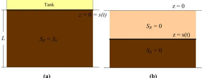
1 Schematic diagram of VOC contamination problem--- 38

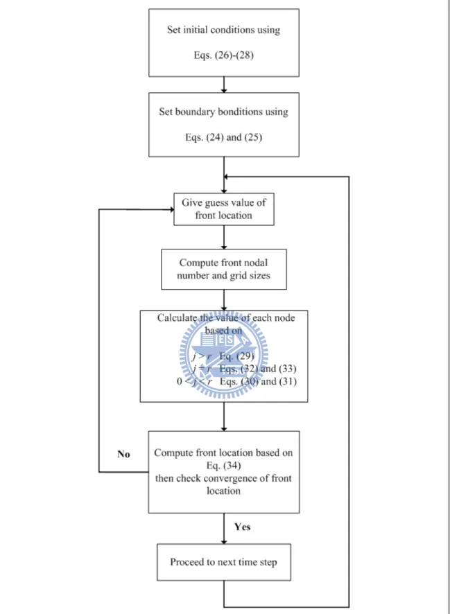
2 Flowchart of the solution procedure for two-component

model--- 39

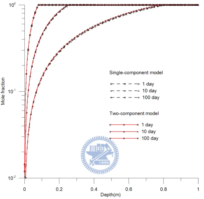
3 Spatial distributions of mole fraction predicted by the

single-component and two-component models at various

evaporation times --- 40

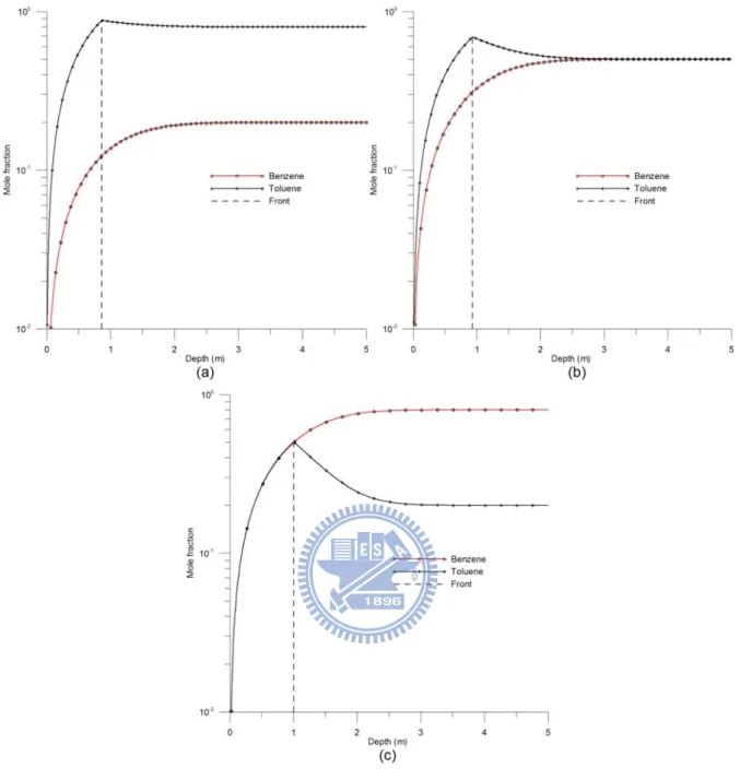
4 The curves of the mole fraction versus depth at 100 day

with various initial mole fractions--- 41

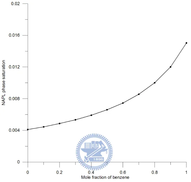
5 NAPL phase saturation versus mole fraction of benzene---- 42

6 Normalized total concentration versus depth at 100 day for

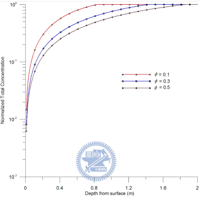
different values of soil porosity --- 43

7 The curves of normalized total concentration versus depth

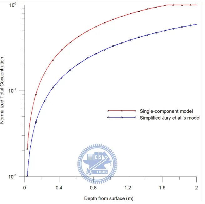
for single-component and simplified Jury et al.’s models at

8

9

10

11

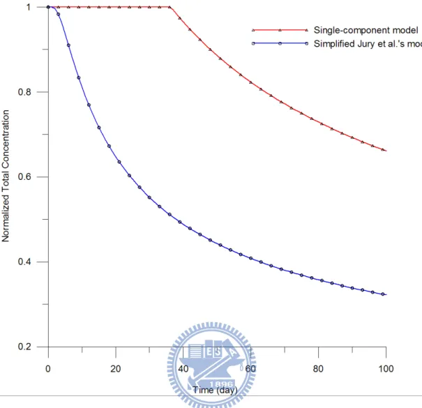
Normalized total concentration versus time for

single-component and simplified Jury et al.’s models at the

depth of 1 m

---Normalized total concentrations of carbon tetrachloride

and toluene versus depth at 100 day

---The curves of the depths of evaporation front versus

evaporation time for carbon tetrachloride and toluene

---Depth and Moving speed of evaporation front versus time

for different effective diffusion coefficients ---45

46

47

48

NOTATION

The following symbols are used in this thesis: CT = total concentration

CL = liquid-phase concentration

CS = adsorbed-phase concentration

CG = gas-phase concentration

CT0 = saturated total concentration

CL0 = saturated liquid concentration

CG0 = saturated gas concentration

CS0 = saturated adsorbed concentration

CGP = equilibrium gas concentrations of pure component

CLP = equilibrium liquid concentrations of pure component

DGair = diffusion coefficient in air

DG = diffusion coefficient in gas phase in soil

DE = effective diffusion coefficient

f = mass fraction of organic compound in NAPL

i = number of component

u = mole fractions of organic compounds in the NAPL phase

u0 = initial mole fraction

φ = soil porosity

θR = volumetric content of NAPL

θL = volumetric content of liquid-phase

θG = volumetric content of gas-phase

θR 0 = initial volumetric content of NAPL

θL 0 = initial volumetric content of liquid-phase

θG 0 = initial volumetric content of gas-phase

SR = saturation of NAPL

SL = saturation of liquid-phase

SG = saturation of gas-phase

S0 = initial NAPL saturation

t = time

z = depth from surface

ρR = density of NAPL

ρb = soil bulk density

KH = Henry’s Law constant

KD = distribution coefficient

Koc = organic carbon partition coefficient

foc = soil organic carbon fraction

PP

0

= saturated vapor pressure of the VOC M = molecular weight of the VOC

T = absolute temperature L = depth of lower boundary

d = stagnant air boundary layer with thickness dz = initial grid size

dzr = grid size above the front dzN-r = grid size below the front

dt = time interval

Uf = moving speed of evaporation front

C = a constant parameter ηi = φSG +

(

)

( )

[

(

)

]

[

(

)

]

CHAPTER 1 INTRODUCTION

1.1

Subsurface contamination by volatile organic compounds (VOCs) has been one of

important issues to environmental problems recently. The pollution of VOCs is a common

problem in nowadays, and VOCs may harm human health in skin and the respiratory system.

The VOCs may enter subsurface soil from a variety of sources such as surface spill and

leaking storage tank. They present in the unsaturated soil in different forms such as gas,

liquid, adsorbed, and non-aqueous phase liquid (NAPL) phases. After a long residing time,

the NAPL phase may be redistributed by water flow and turn into residual phase which is

essentially held by surface tension and may stay in the soil pores over a long period of time.

The transport mechanisms of VOC in the unsaturated soil generally include advection,

diffusion, dispersion, adsorption, volatilization, and chemical and biological reactions.

Often diffusion is the dominating mechanism under natural condition, especially, for gas

transport in a low-permeability soil. Advection is commonly ignored in studying organic

vapor and gas migration in unsaturated soils (e.g., Jury et al., 1983; Zaidel and Russo, 1994;

Yates et al., 2000). Falta et al. (1989) indicated that density driven advection is insignificant

if the magnitude of soil permeability is less than 1×10-11 m2. Massmann and Farrier (1992)

mentioned that the advection induced by atmospheric fluctuation is not substantial for gas

conditions.

Soil vapor extraction (SVE) is an in-situ remedial technology for removing volatile

constituents from unsaturated contaminated soils. In the cases of sparse VOC or low

permeability formation, the removal efficiency of volatile compounds in soils will be

significantly decreased. For this reason, diffusion may be the dominating mechanism for

VOCs to move to a high permeability zone or volatilize to atmosphere under natural condition

(Hoier et al., 2007). For nature evaporation, the upper boundary of the zone having NAPL

phase becomes a front which moves downward with increasing time. The evaporation front

of NAPL phase can therefore be defined as a moving boundary and the location of the moving

boundary naturally represents the depth of NAPL. Moving boundaries are time-dependent

and the position of the boundary has to be determined as a function of time and space (Crank,

1984). The moving boundaries occur mostly in heat-flow problems with phase changes and

in some diffusion problems.

1.2 Literature Review

Jury et al. (1983) presented an analytical solution for a single pesticide species without

NAPL phase undergoing first-order decay in an unsaturated zone. Sleep and Sykes (1989)

presented a two-dimensional finite element model to simulate VOC partitioning to gas, liquid,

solid and NAPL phases and its transport in unsaturated soils. They indicated that the

al. (1990) used a method developed by Jury et al. (1983) to study the effect of vapor phase

sorption on organic compounds transport. Their results showed that vapor phase sorption

affects liquid phase organic concentration and also retards the rate of chemical migration

toward the water table. Massmann and Farrier (1992) proposed a mathematical model to

describe the transport of organic compounds in NAPL, gas, liquid, and adsorbed phases and

used the finite difference approximation to simulate the movement of contaminants emanating

from two point sources. Zaidel and Zazovsky (1999) developed a mathematical model to

investigate the depletion of multi-component NAPL due to the evaporation and vapor

transport in a SVE process. Yates et al. (2000) presented an analytical model to study the

diffusion of organic vapors or other gases in layered soil systems.

Moving boundary problems are also called Stefan problems referred to Stefan’

investigations on the melting of the polar ice cap (Stefan, 1889a and b). Crank (1984) gave a

literature survey on the Stefan problems occurring in physical and biological sciences,

engineering, and decision and control theory, etc. Recently, studies involved moving

boundaries were applied in the areas such as heat conduction [e.g., Cheng, 2000],

solidification and melting processes [e.g., Feltham and Garside, 2001; Szimmat, 2002;

Caldwell et al., 2003; Lee and Marchant, 2004; Rattanadecho, 2006; Naaktgeboren, 2007;

Patnaik et al., 2009], dissolution [e.g., Quintard and Whitaker, 1995; Vazquez-Nava and

1.3 Objectives

The purpose of this thesis is to develop a two-component model to predict the mole

fraction distributions of VOC and the migration of evaporation front of NAPL phase after the

removal of the storage tank in a homogeneous unsaturated soil. To the best of our

knowledge, the existing models in simulating the natural evaporation of VOC in unsaturated

soil have the problem domains all with fixed boundaries. In contrast, the present model

considers a moving boundary to describe the downward move of evaporation front of NAPL

phase. The front, which migrates downward with time, is treated as a lower boundary while

the land surface is used as the upper boundary for the region above the front. For the region

below the front, the front becomes the upper boundary and the lower boundary is located at

some distance below the land surface. Based on the present model with these boundaries,

VOC mole fraction distributions and the front location are solved by the finite difference

method with a moving grid approach. This numerical model can predict the mole fraction

distributions between two components and the movement of the front, analyze evaporation

time of VOC, and assess the influences of initial mole fraction, soil porosity as well as

chemical volatility on VOC migration in the unsaturated soil. Moreover, a

single-component model is obtained from simplifying the two-component model and solved

analytically using Boltzmann’s transformation. Then, an analytical expression for the

CHAPTER 2 METHMETICL MODEL

This chapter presents the mathematical models and related solution procedures for VOC

transport in homogeneous and unsaturated soils.

2.1. Mathematical model: Two-component case

Figure 1(a) shows a leaking storage tank located on the top of land surface and filled

with VOC. Consider that the VOC leaking from the tank has four different phases (namely,

gas, liquid, adsorbed and residual NAPL phases) and distributes uniformly in the unsaturated

zone. Each phase has a saturated or equilibrium concentration and constant volumetric

content. The VOC has an initial NAPL saturation S0 in the soil. The saturation of each

phase denotes as the volume percentage in the soil pore and the sum of saturation of each

phase equals one. The evaporation front of the NAPL, denoted as s(t), initially stays right at

the land surface, i.e., z = s(t) = 0 where z is the vertical axis, and moves downward with

increasing time. Figure 1(b) shows the contamination scenario in which the gas phase VOC

begins to evaporate to atmosphere and the NAPL starts to vaporize to gas phase after the tank

being removed. Assume that the NAPL phase of VOC evaporates fully above the front and

the front migrates instantaneously when the evaporation occurs. In other words, the VOC

presents only in gas, liquid, and adsorbed phases and the NAPL saturation, SR, equals zero

between the land surface and the front. Below the front, the residual VOC still exists. At

of NAPL transferring to gas phase follows the conservation of mass.

The total concentration of VOC is the sum of the concentration of each phase; that is:

R R b S L L G G T C C C C = θ + θ + ρ +ρ θ (1) where CG, CL, and Cs represent the chemical concentrations in the gas, liquid, and adsorbed

phases, respectively, and ρb and ρR are the soil bulk density and density of NAPL,

respectively. The symbols θG, θL, and θR are the volumetric contents of gas, liquid, and

NAPL phases, respectively, and denote as

G G φS

θ = , θ_L =φS_L, and θ_R =φS_R (2)

where φ is the soil porosity and SG and SL are gas and liquid saturations, respectively.

The equilibrium relationships between the gas and liquid phases as well as the liquid and

adsorbed phases may be expressed, respectively, as

L H G K C

C = and C_S =K_DC_L =K_ocf_ocC_L (3)

where KH is Henry’s Law constant, KD is the distribution coefficient, Koc is the organic carbon

partition coefficient, and foc is the soil organic carbon fraction. The equilibrium relationships

given in Equation (3) are linear and reversible and their coefficients are dependent on

different chemical characteristics and soil properties.

The equation of mass conservation for those four phases in the unsaturated soil is

[

]

tortuosity factor accounting for the reduced flow area and increased path length of diffusing

molecules in soil can be related to the soil porosity and the fluid content in the soil.

Millongton and Quirk (1961) defined that

⎟ ⎟ ⎟ ⎠ ⎞ ⎜ ⎜ ⎜ ⎝ ⎛ = ₂3 10 φ θ_G air G G D D (5)

where DGair is the air-gas diffusion coefficient.

Consider that VOC has multiple components. Substituting Equations (2) and (3) into

Equation (4), the mass-conservation equation in three dimension for those four phases in the

unsaturated soil becomes (Zaidel and Zazovsky, 1999)

(

)

[

]

(

)

∑

∑

∑

where and are equilibrium gas and liquid concentrations of pure component,

respectively, f is the mass fraction of organic compound in NAPL, i is the number of each

component, and N p G C p L C

concentration for pure component can be estimated from the idea gas law as T M P CP G = /ℜ 0 (9) where PP

0 _{is the saturated vapor pressure of the VOC, M is the molecular weight of the VOC,}

is the ideal gas constant, and T is the absolute temperature. ℜ

To describe the behavior of volatilization of VOC from NAPL phase to gas phase, the

evaporation front is introduced as a moving boundary in the unsaturated soil. The problem

domain for VOC transport with a moving boundary in the soil can be divided into three

regions. The VOC transport equations in these three regions are described below.

2.1.1 Below the evaporation front

In this region, NAPL phase exists and the saturation of NAPL phase is greater than zero, i.e., S_R >0. Equation (8) can then be expressed as

1 1 =

∑

with representing mole fractions of organic compounds in the NAPL phase, i.e.,

. For a one-dimensional system, Equation (6) becomes:

i u P Gi Gi i C C u = /

(

)

∑

where η_i =φS_G+

(

)

based on Equation (11), the mass-conservation equation for each component can be written

P Gi R i ρ φ/C

as:

(

)

(

)

Select u = u1 as a primary variable. The saturation of NAPL phase can be obtained from

Equation (12) as

(

)

[

]

[

(

)

]

(

)

where δ_i =η_i/D_G, μ_i =σ_iM /_i D_G, and C is a constant parameter computed by the initial NAPL saturation S0 and mole fraction u0 of component one as:

) 1 ( ) 1 ( ) 1 ( ₀ 2 0 1 0 2 0 1 0 0 2 0 1 u M u M u u S u u C − + − + + − + =δ δ μ μ (15)

Substituting Equations (10) and (14) into Equation (12) yields

( )

( )

[

(

)

]

[

(

)

]

2.1.2 Above the evaporation front

In this region the NAPL phase fully evaporates. i.e., S_R =0. For a two-component VOC, Equation (11) can be written for each component as follows:

2 1 2 1 1 z u t u ∂ ∂ = ∂ ∂ δ (17) 2 2 2 2 2 z u t u ∂ ∂ = ∂ ∂ δ (18)

where u1 and u2 represent normalized concentrations above the evaporation front,

2.1.3 At the evaporation front

Assume that the evaporation of NAPL phases occurs instantaneously and the sum of

mole fraction equals one, i.e., u1+u2 = 1. Combining Equations (12) and (13), the equation

for mass conservation at the front can be expressed as

t u t u z u D z u D t S_{R G G} ∂ ∂ ⎟⎟ ⎠ ⎞ ⎜⎜ ⎝ ⎛ − ∂ ∂ ⎟⎟ ⎠ ⎞ ⎜⎜ ⎝ ⎛ − ∂ ∂ ⎟⎟ ⎠ ⎞ ⎜⎜ ⎝ ⎛ + ∂ ∂ ⎟⎟ ⎠ ⎞ ⎜⎜ ⎝ ⎛ = ∂ ∂ 2 2 2 1 1 1 2 2 2 2 2 1 2 1 σ η σ η σ σ (19)

Taking the limits of and , Equation (18) describing the front can then be

written as 0 → Δt Δz→0

(

)

(

)

where the superscripts t+ and t– of the mole fraction in Equation (20) denote the mole fraction

at the time slightly after and before the volatilization, respectively, and z+ and z– represent the

mole fraction at the region slightly below and above the front, respectively. Equation (20)

can be further simplified as

(

)

(

)

2.1.4 Boundary and initial conditions

considered to diffuse across a stagnant air boundary layer with thickness d and the gas phase

concentration is assumed equal to zero at the top of boundary layer. The flux diffusing to

the atmosphere can then be expressed as (Jury et al., 1983)

G T G G R C h z C D = ∂ ∂ , at z=0 (22)

where . If the thickness of air boundary layer near the surface is very small and

negligible, one may assume that d = 0. Equation (22) can then be expressed as d D h air G / = 0 = T C , at z=0 (23)

For a multicomponent VOC, the upper boundary conditions can be written from Equation (23)

as

( )

( )

u ₍₂₄₎

The conditions of the mole fractions at the lower boundary are denoted as:

( )

u₁ , = , u₂

( )

where L is the depth of the lower boundary.

The initial NAPL saturation and the mole fractions of each component are assumed

spatially uniform; they are

( )

S_R = (26)

( )

The evaporation front is initially located at the land surface and thus denoted as

( )

s (28)

2.2 The numerical method in solving the model

This section presents the numerical method used to solve the two-component model.

2.2.1 Finite difference approximation

The equations of describing VOC transport in the three regions are solved separately by

the finite difference method. An interpolative moving grid approach (Javierre et al. 2006) is

adopted to handle the moving boundary problem. The total number of nodes within the

problem domain is equal to N and r is the nodal number assigned at the evaporation front

beginning from the land surface. Accordingly, the number of grids from the land surface to

the front is r-1, the number of grids below the front is N-r, and the initial grid size dz is equal

to L/(N-1). The grid sizes above and below the front defined as dzr and dzN-r, respectively,

need to be re-estimated after each move of the front. To avoid introducing large truncation

error, the grid sizes dzr and dzN-r should be close to dz. If the front move to a location

between the nodal numbers initially assigned as j and j+1, the new grid sizes of dzr and dzN-r

are then estimated by s/(r-1) and (L-s)/(N-r), respectively, where r = j+1. The backward

difference relative to time and central difference relative to space are used to approximate the

region below the front obtained from Equation (16) is

( ) ( )

where n is the number of time step, and dt is the time interval. The difference equations for

the mole fractions of the two components in the region above the front obtained from

Equations (17) and (18) are, respectively:

2 ) 1 ( 1 1 ) 1 ( 1 1 1 1 1 ) ( 2 r n j n j n j n j n j dz u u u dt u u − _{+ − + −} = − δ , 0≤z<s(t) (30) 2 ) 1 ( 2 2 ) 1 ( 2 1 2 2 2 ) ( 2 r n j n j n j n j n j dz u u u dt u u − _{+ − + −} = − δ , 0≤z<s(t) (31)

Finally, the difference equations for the mole fractions of the two components at the

front also derived from Equations (17) and (18) with different grid sizes above and below the

front are, respectively, expressed as

r N r r N r n r r N r n r r N n r r n r n r dz dz dz dz u dz dz u dz u dz dt u u − − − − − + − + + − + = − ⎟ ⎠ ⎞ ⎜ ⎝ ⎛ ) ( ) ( 2 1 ) 1 ( 1 ) 1 ( 1 1 1 1 1 δ , z=s(t) (32) r N r r N r n r r N r n r r N n r r n r n r dz dz dz dz u dz dz u dz u dz dt u u − − − − − + − + + − + = − ⎟ ⎠ ⎞ ⎜ ⎝ ⎛ ) ( ) ( 2 2 ) 1 ( 2 ) 1 ( 2 1 2 2 2 δ , z=s(t) (33)

Substituting Equation (10) into Equation (21), the difference equation for the front location

(

)

(

)

2.2.2 The solution procedure of the model

Because the location of the evaporation front s(t) is unknown, a trial and error procedure

is therefore taken to find the front location. The steps of the procedure are listed below and

the related flowchart is shown in Figure 2:

1. Give the initial front location (Equation (28)) and nodal values of mole fraction based on

the boundary conditions (Equations (24) and (25)) and initial conditions (Equations (26) and

(27)).

2. Guess front location after the start of evaporation.

3. Determine the nodal number for the front and the grid sizes based on the front location.

4. Solve the solutions for the region below the front (Equation (29)), for the region above the

front (Equations (30) and (31)), and at the front (Equations (32) and (33)).

5. Compute the front location based on Equation (34).

6. Proceed to next time step if the location of the front converges, i.e., the difference between

two succeeding estimations of the front location is less than a very small value, e.g., 10-10 m;

2.3 Simplified model: Single-component case

This section presents a single-component model with the governing equation simplified

from the two-component model. The domain of the single-component model is also divided

into three regions based on the front location. In a one-dimensional homogeneous and

unsaturated soil system, Equation (6) representing the VOC transport can be written as

0 2 2 = ∂ ∂ − ∂ ∂ z C D t C _G G T ₍₃₅₎

2.3.1 Below the evaporation front

In this region, the NAPL has not vaporized to gas phase yet. The VOC concentrations

in each phase are the initial saturated concentrations and the total concentration can be

expressed as 0 0 0 0 R R b P S L P L G P G T T C C C C C = = θ + θ + ρ +ρ θ (36) where CSP is the saturated VOC concentrations for pure component in adsorbed phases, CT0 is

the initial total concentration, and θG0, θL0, and θR0 are the initial volumetric contents,

respectively.

2.3.2 Above the evaporation front

In this region, NAPL phase of the VOC completely vaporizes to gas phase; therefore, the VOC presents only in gas, liquid, and adsorbed phases, i.e., CT = CGθG+ CLθL+CSρb. Jury et

Accordingly, one may introduce the following equation based on Equations (1) and (3): S S L L G G T R C R C R C C = = = (37)

where the ratios are R_G =θ_G+θ_L K_H +ρ_bK_D K_H , R_L =θ_GK_H +θ_L +ρ_bK_D, and

b D L D H G S K K K R =θ +θ +ρ .

With Equation (37), Equation (35) can be written as

0 2 2 = ∂ ∂ − ∂ ∂ z C D t C _T E T ₍₃₈₎

where denotes as effective diffusion coefficient. Equation (38) describes the

VOC transport in gas and liquid phases between the land surface and evaporation front. In

reality, the volatilization of NAPL occurs right at the evaporation front which will be

discussed in the next section.

G G E D R

D = /

2.3.3 At the evaporation front

The evaporation front moves downward while the NAPL vaporizes to the gas phase.

Assume that the transformation of the contents between these two phases occurs

instantaneously and the liquid volumetric content is unchanged, i.e., θL = θL0. In addition,

the VOC concentrations in each phase are still saturated,i.e., CG = CGP, CL = CLP, and CS =

CSP. The total concentration at the front can therefore be expressed as

0 T T C

C = (39)

θR equals soil porosity φ, i.e., θG+θL+θR =φ. Assumes φ does not change with time,

the transformation of volumetric content with respect to time among each phase is conserved.

Thus, t t t R L G ∂ ∂ − = ∂ ∂ + ∂ ∂θ θ θ (40)

Since ∂θ_L/∂t =0, one can get ∂θ_G/∂t=−∂θ_R/∂t from Equation (40). In addition, the bulk density ρb does not change with time, i.e., ∂ρb/∂t =0. Therefore, one can obtain the

following relationship from Equation (1)

(

)

With Equation (41) and taking the limits of Δt→0 and Δz→0, Equation (35) describing

the front can then be written as

(

)

where the superscripts + and - denote the volumetric content at the time slightly after and

before the volatilization, respectively, and the concentrations at the region slightly below and

above the front, respectively. Consider that the volatilization occurs instantaneously,

therefore equals and equals zero after evaporation. The VOC

concentrations in each phase are the initial saturated concentrations below the front and the

concentration gradient of gas phase below the front is naturally equal to zero, i.e.,

+ R θ 0 R θ − R θ 0 = ∂ ∂ + z

orders (Falta et al., 1989, Tables 1 and 4), the term related to CGP on the left-hand side of

Equation (42) is thus negligible. Accordingly, Equation (43) representing the front z = s(t)

can be expressed as z C D dt ds _T E R R _∂ ∂ = − ρ θ0 (43)

2.3.4 The analytical solution of single-component model

Consider that the VOC is saturated or in equilibrium state in different phases and

uniformly distributed in the unsaturated soil initially. The mathematical model describing

the single-component VOC transport in the soil consists of Equation (38) as the governing

equation, Equations (39) and (43) as the lower boundary conditions, and Equation (23) as the

upper boundary condition.

Based on Boltzmann’s transformation, a new variable is defined as ξ = z 2 D_Et . Equation (38) can then be transformed to an ordinary differential equation as

0 2 2 2 = + ξ ξ ξ d dC d C d _{T T} (44)

The solution of Equation (44) can be obtained as (Carslaw and Jaeger, 1959)

( )

A

C_T(ξ)= ⋅ ξ + (45) where erf(ξ) is the error function and A and B are unknown coefficients. Substituting Equation (45) into Equation (23), the result for the concentration distribution is

( )

Substituting Equation (39) into Equation (46), the evaporation front s(t) and coefficient A

can then be obtained, respectively, as

t t s( )=α (47) ⎟ ⎟ ⎠ ⎞ ⎜ ⎜ ⎝ ⎛ = E T D erf C A 2 0 α (48)

where α is an unknown constant depending upon the soil parameters and contaminant

characteristics.

The time of vanish of NAPL can be solved by Newton’s method (Yeh, 1987) from

Equation (47) when the front reaches a target location below the land surface designated by

the environmental or legal requirement. In addition, the moving speed of the evaporation

front can also be obtained after taking the derivative of Equation (47) with respect to time and

the result is t U_f 2 α = (49) Substituting Equations (46), (47) and (48) into Equation (43) yields

⎟ ⎟ ⎠ ⎞ ⎜ ⎜ ⎝ ⎛ ⎟⎟ ⎠ ⎞ ⎜⎜ ⎝ ⎛ − = E E E T E R R D erf D D C D 2 4 exp 2 2 0 0 α π α α ρ θ (50)

The unknown constant α can then be easily determined from Equation (50) by Newton’s

method. Note that the normalized total concentration is defined as CT(z,t)/CT0, representing

CHAPTER 3 RESULTS AND DISCUSSION

Leaks of petroleum fuels from the underground storage tanks are common problems for

soil contamination. The petroleum spills are often associated with aromatic hydrocarbons

such as benzene, toluene, ethyl benzene, and various xylene isomers (BTEX). In this section,

the hydrocarbons of benzene and toluene are chosen to simulate their transport and mole

fraction distributions in unsaturated soils using the two-component model. In the past,

Carbon tetrachloride was commonly used as coolant in industry or produced as the fire

extinguishers. Carbon tetrachloride is highly toxic; a small amount of this chemical residing

in the soil may pose severe environmental problems. The carbon tetrachloride in the

unsaturated soil is considered as a target VOC and analyzed using the single-component

model.

Six cases are considered to address the issues in regard to the evaporation rate,

evaporation front movement, mole fraction, and concentration distributions of VOC for the

present models. Case 1 is to compare the mole fractions of toluene at various evaporation

times predicted by single-component and two-component models. Case 2 examines the

effect of initial mole fraction on the evaporation and the changes of the mole fraction

distributions of benzene and toluene. Case 3 investigates the effect of soil porosity on

vaporization of carbon tetrachloride from NAPL phase to gas phase while case 4 addresses

the presence of NAPL phase. Case 5 studies the migrations of evaporation front for different

contaminants, namely carbon tetrachloride and toluene. Case 6 discusses the effect of

effective diffusion coefficient of carbon tetrachloride on the moving speed of evaporation

front. The values of the soil chemical properties are listed in Table 1 and the properties of

benzene, toluene, and carbon tetrachloride are given in Table 2 for these six cases. Note that

the depth of the lower boundary L is chosen as 5 m, the total number of nodes N is 10000, and

the time interval dt is 0.1 sec in the case study when adopting the finite different

approximation for the two-component model.

3.1 Case 1: Different evaporation times in two models

This case uses the same assumptions for both single-component and two-component

models and considers that toluene is the only VOC found in the soil, i.e., u0 = 1. Figure 3

shows the mole fraction distributions of toluene versus depth predicted by the

single-component and two-component models at various evaporation times. The dashed line

denotes the solution of single-component model while the solid line represents the results

predicted by the two-component model. Moreover, the symbols of rhombus, triangle, and

circle represent the mole fractions at times 1, 10, and 100 day, respectively. This figure

shows the front locations at various evaporation times and at the front the mole fraction equals

its initial value for the single-component VOC. The figure also shows that the curves

two-component model with the present numerical approach match well with those estimated

based on the analytical solution of the single-component model. The moving speeds of the

front Uf estimated by equation (49) are 8.296×10-2, 2.624×10-2, and 8.296×10-3 m/day at times

1, 10, and 100 day, respectively, indicating that the moving speed decreases rapidly at early

time and then slowly as time increases

3.2 Case 2: Initial mole fraction

In this case, benzene is considered to be component one and toluene is component two in

the two-component model. Figures 4(a) - 4(c) show the mole fraction distributions of

benzene and toluene versus depth when the initial mole fractions of component one are 0.2,

0.5, and 0.8, respectively, at 100 day. The evaporation front of the NAPL with u0 = 0.2, 0.5,

and 0.8 reaches 0.860, 0.931, and 1.002 m below the surface, respectively. In addition, at

the front u1 = 0.123 and u2 = 0.877 when u0 = 0.2, u1 = 0.310 and u2 = 0.690 when u0 = 0.5,

and u1 = 0.498 and u2 = 0.502 when u0 = 0.8. The figures show that the depth of the front

increases with the initial mole fraction of benzene, representing the moving speed of the front

depends on the initial mole fraction. The mole fraction of benzene increases with depth until

reaching u1 = u0; on the other hand, the mole fraction of toluene increases above the front but decreases below the front until reaching u₂ =1 u− ₀. These results indicate that at the front, the mole fraction of benzene decreases as time increases while that of toluene increases with

the front. In fact, both components reach their initial values occurred at certain distances

below the front. Such a phenomenon can be attributed to the fact that benzene has higher

evaporation efficiency than toluene. Therefore, the mole fractions of benzene and toluene

change with depth, although the NAPL below the front does not evaporate. Figure 5 shows

the curve of NAPL phase saturation, calculated from Equation (14), versus mole fraction of

benzene. The figure demonstrates that SR equals 0.004 when u0 = 0 and 0.015 when u0 = 1.

This result indicates that SR changes with mole fraction and varies slightly below the front.

3.3 Case 3: Soil porosity

This case examines the effect of soil porosity on the concentration distribution of carbon

tetrachloride using the single-component model. The total evaporation time is considered to

be 100day. Note that the saturation S of each phase is constant and the volumetric contents

θ of gas, liquid, and NAPL change in equal proportion with the soil porosity. Figure 6 shows the predicted normalized total concentration versus depth at 100 day for the porosities

of 0.1, 0.3, and 0.5. It is apparent from Figure 4 that the vaporization increases moderately with soil porosity. In addition, the evaporation front of the NAPL with φ = 0.1, 0.3, and 0.5 are at 0.831, 1.432, and 1.860 m below the land surface, respectively, and the moving

speeds of the front are 4.154×10-3, 7.158×10-3, and 9.301×10-3 m/day, respectively, indicating

that the moving speed of the front increases with soil porosity although different amounts of

3.4 Case 4: Absence of the NAPL phase

In this case, the effects of presence and absence of NAPL on the distribution of carbon

tetrachloride in the soil are compared and studied. Jury et al. (1983) considered the scenario

that there were three phases of VOC presented in the soil with neglecting the NAPL phase.

Their analytical model included the mechanisms of diffusion, soil water advection, and

first-order decay. They used a diffusive flux as the upper boundary condition at the land

surface and zero total concentration at infinite depth as the lower boundary condition. Jury

et al.’s model is simplified by neglecting the water phase advection and decay and thus called

simplified Jury et al.’s modelhereafter.

Figure 7 shows the curves of normalized total concentration of carbon tetrachloride

versus depth predicted by two different VOC transport models at t = 100 day. The solid line

with triangle symbol represents the normalized total concentration distribution predicted by

the present single-component model while the solid line with circle predicted by simplified

Jury et al.’s model. Figure 7 indicates that the normalized total concentration of VOC

predicted by the present model is significantly higher than that of simplified Jury et al.’s

model. Although NAPL occupies only one-percent of volume in the soil pores, the NAPL

however affects the total concentration distribution and transport capability greatly. Figure 8

exhibits the predicted distribution of normalized total concentration versus time for the

the total concentration of carbon tetrachloride decreases quickly after 2 day predicted by

simplified Jury et al.’s model and after 37 day by the single-component model indicating that

the presence of NAPL has significant impact on the VOC transport.

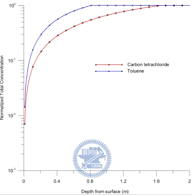
3.5 Case 5: Different chemicals

In this case, both carbon tetrachloride and toluene are considered to reside in the

unsaturated soil. Table 2 shows that toluene has less molecular weight and liquid density

and lower saturated vapor pressure and Henry’s law constant than those of carbon

tetrachloride. Figure 9 shows the curves of normalized total concentration versus depth for

carbon tetrachloride and toluene at 100 day predicted by the single-component model for each

chemical. The solid lines with circle and triangle represent the concentration distributions of

carbon tetrachloride and toluene, respectively. The vaporization of toluene is significantly

lower than that of carbon tetrachloride; the depths of the evaporation front of carbon

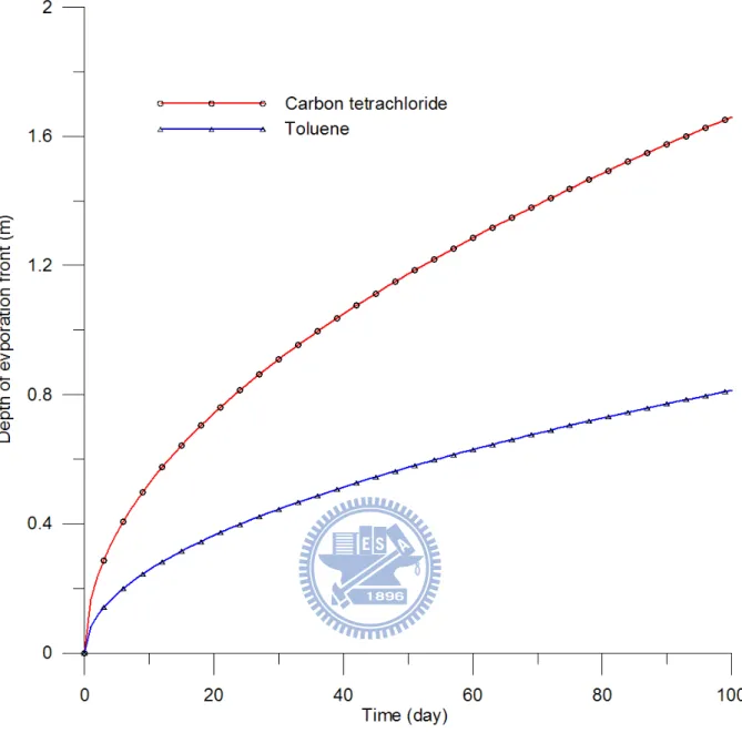
tetrachloride and toluene equal 1.659 m and 0.813 m, respectively, at 100 day. Figure 10

shows that the depths of the front versus evaporation time for both chemicals. This figure

indicates that the fronts at 50 day and 100 day reach the depths of 1.173 m and 1.659 m,

respectively, for carbon tetrachloride and 0.575 m and 0.813 m, respectively, for toluene.

Obviously, the migration of the front of carbon tetrachloride is significantly faster than that of

toluene due to lower vapor pressure and Henry’s Law constant value of toluene. Such a

and liquid phases. In addition, the diffusion coefficients of gas and liquid phases of both

chemicals differ by four orders of magnitude. Thus the diffusion of liquid phase is

significantly lower than that of gas phase.

3.6 Case 6: Effect of effective diffusion coefficient on moving speed of evaporation front

Equation (49) shows the moving speed of evaporation front Uf which in fact represents

the evaporation rate of NAPL in soil. This case investigates the effect of the soil chemical

properties on Uf based on the single-component model. The DE is a function of soil porosity,

volumetric content of each phase, air diffusion coefficient, soil bulk density, Henry’s Law

constant, and organic carbon fraction. Obviously, different soil chemical properties will

affect the value of DE. Figure 11 shows the curves of the depth and moving speed of the

front versus evaporation time for DE = 10-10, 10-9, 10-8, and 10-7 m2/s. The depth of the front

increases with time and DE greatly while the moving speed is maximal when VOC begins to

CHAPTER

4 CONCLUSIONS

This thesis presents a two-component model to describe the mole fraction distributions

of VOC in the unsaturated soil. In the model, zero-concentration is chosen as the upper

boundary condition and a moving boundary representing the evaporation front of NAPL is the

lower boundary in the region where the NAPL evaporates fully. In the region below the

front, the NAPL phase prevails. The upper boundary of this region is the evaporation front

and the lower boundary is relatively far away from the front and thus chosen at infinity. The

model is solved by the finite difference method with a moving grid approach. This

numerical model is applied to predict the mole fraction distributions between two components

and the movement of the front in the soil. In addition, the numerical model is also used to

analyze evaporation time of VOC and assess the influences of initial mole fraction, soil

porosity as well as chemical volatility on VOC migration. The two-component model is

further simplified to a single-component model, which is solved analytically based on

Boltzmann’s transformation. In addition, analytical expressions are also developed for the

front and its moving speed as functions of evaporation time, characteristics of soil and VOC,

and volumetric content of each phase.

Both two-component and single-component models have been used to study the problems

of the evaporation rate, evaporation front movement, mole fraction, and concentration

following conclusions can be drawn:

1. The VOCs such as benzene and toluene usually have different transport efficiencies. The

predicted results from the two-component model indicate that the initial mole fraction of

each component has affects on the location of evaporation front and the mole fraction

distributions. As the result, the depth of the front increases with the initial mole fraction

for benzene but decreases with that for toluene.

2. The NAPL distributions after evaporation for single-component and two-component VOCs

are different. For the single-component case, the total VOC concentration at or below the

front is always equal to the initial concentration; however, for two-component case the

mole fractions of VOC at the front will change with time base on different evaporation

efficiencies of two components. In other words, both the mole fractions and NAPL phase

saturation change with depth below the front for a two-component VOC.

3. The migration distance of the evaporation front of NAPL increases with evaporation time

and soil porosity. As a result, the NAPL phase will vaporize to gas phase and vanishes

slowly with increasing time.

4. The normalized total concentration of VOC in the case without the presence of NAPL will

be significantly lower than that with the presence of the NAPL. Even if the volumetric

5. Gas phase diffusion is the dominating transport mechanism for VOC migration in the

unsaturated soil. Since Toluene has lower values of vapor pressure and Henry’s Law

constant than those of carbon tetrachloride, the migration of the evaporation front of

toluene is therefore significantly slower than that of carbon tetrachloride.

6. Both the depth and moving speed of evaporation front increase with the effective diffusion

coefficient. Moreover, the depth of the front increases with time while the moving speed

References

Baehr, A. L., 1987. Selective transport of hydrocarbons in the unsaturated zone due to

aqueous and vapor phase partitioning. Water Resour. Res. 23 (10), 1926-1938.

Caldwell, J., Kwan, Y.Y., 2003. On the perturbation method for the Stefan problem with

time-dependent boundary conditions. Int. J. Heat Mass Transfer. 46, 1497–1501.

Cheng, T.F., 2000. Numerical analysis of nonlinear multiphase Stefan problem. Comput. Struct. 75, 225-233.

Carslaw, H. S., Jaeger, J. C., 1959. Conduction of heat in solids. 2nd ed., Clarendon, Oxford,

Corapcioglu, M.Y., Baehr, A.L., 1987. A compositional multiphase model for groundwater

contamination by petroleum products. Water Resour. Res. 23(1), 191-200.

Crank, J., 1984. Free and moving boundary problems. Oxford Univ. Press, New York,

Falta, R. W., Javandel, I., Pruess, K., Witherspoon, P. A., 1989. Density-driven flow of gas

in unsaturated zone due to evaporation of the volatile organic compounds. Water Resour. Res. 25(10), 2159-2169.

Feltham, D.L., Garside, J., 2001. Analytical and numerical solutions describing the inward

solidification of a binary melt. Chem. Eng. Sci. 56, 2357-2370.

Fetter, C.W., 1993. Contaminant hydrogeology. Prentice Hall, New Jersey.

Experimental investigation of pneumatic soil vapor extraction. J. Cont. Hydrol. 89,

29-47.

Javierre, E., Vuik, F.J., Vermolen, S., Zwaag, van der, 2006. A comparison of numerical

models for one-dimensional Stefan problems. J. Comput. Appl. Math. 192, 445-459.

Jury, W. A., Spencer, W. F., Farmer, W. J., 1983. Behavior assessment model for trace

organics in soil: I. Model description. J. Environ. Qual. 12 (4), 558-564.

Jury, W., A., Russo, D., Streile, G., EL Abd H., 1990. Evaluation of volatilization by organic

chemicals residing below the soil surface. Water Resour. Res. 26 (1), 13-20.

Lee, M.Z.C., Marchant, T.R., 2004. Microwave thawing of cylinders. Appl. Math. Modell.

28, 711–733.

Massmann, J., Farrier, D., 1992. Effects of atmospheric pressure on gas-transport in the

vadose zone. Water Resour. Res, 28(3), 777-791.

Millongton, R. J., Quirk, J. M., 1961. Permeability of porous solids. Trans. Faraday Soc. 57,

1200-1207.

Naaktgeboren, C., 2007. The zero-phase Stefan problem. Int. J. Heat Mass Transfer. 50,

4614–4622.

Patnaik, S., Voller, V.R., Parker, G., Frascati, A., 2009. Morphology of a melt front under a

Perry, R. H., Green, D.W., Maloney, J.Q., 1997. Perry’s chemical engineers’ handbook. 7th

ed., McGraw-Hill, New York.

Pinder, G. F., Abriola, L. M., 1986. On the simulation of nonaqueous phase organic

compounds in the subsurface. Water Resour. Res. 22 (9), 109S-119S.

Purlis, E., Salvadori, V.O., 2009. Bread baking as a moving boundary problem. Part 1:

Mathematical modelling. J. Food Eng. 91, 428–433.

Purlis, E., Salvadori, V.O., 2009. Bread baking as a moving boundary problem. Part 2:

Model validation and numerical simulation. J. Food Eng. 91, 434–442.

Quintard, M., Whitaker, S., 1995. The mass flux boundary condition at a moving fluid-fluid

interface. Ind. Eng. Chem. Res. 34, 3508-3513.

Rattanadecho, S., 2006. Simulation of melting of ice in a porous media under

multipleconstant temperature heat sources using a combined transfiniteinterpolation and

PDE methods. Chem. Eng. Sci. 61, 4571–4581.

Sazhin, S.S., Krutitskii, P.A., Gusev, I.G., Heikal, M.R., 2010. Transient heating of an

evaporating droplet. Int. J. Heat Mass Transfer. 53, 2826–2836.

Shoemaker, C. A., Culver, T. B., Lion, L. W., Peterson, M. G., 1990. Analytical models of

the impact of two- phase sorption on subsurface transport of volatile chemicals. Water Resour. Res. 26 (4), 745-758.

Sleep, B. E., Sykes, J. F., 1989. Modeling the transport of volatile organics in variably

saturated media. Water Resour. Res. 25 (1), 81-92.

Stefan, J., 1889. Sber. Akad. Wiss. Wien. 98, 473-484.

Stefan, J., 1889. Sber. Akad. Wiss. Wien. 98, 965-983.

Szimmat, J., 2002. Numierical simulation of solidification processes in enclosures. Heat and Mass Transfer. 38, 279-293.

Vazquez-Nava, E., Lawrence, C., Thermal dissolution of a spherical particle with a moving

boundary. Heat Transfer Eng. 30(5), 416–426.

Yates, S. R., Papieri, S. K., Gao, F., Gan, J., 2000. Analytical solutions for the transport of

volatile organic chemicals in unsaturated layered systems. Water Resour. Res. 36(8),

1993-2000.

Yeh, H. D., 1987. Theis' solution by nonlinear least-squares and finite- difference Newton's

method, Ground Water. 25(6), 710-715.

Zaidel, J., Russo, D., 1994. Diffusive transport of organic vapors in the unsaturated zone

with kinetically-controlled volatilization and dissolution: analytical model and analysis. J. of Contam. Hydro. 17, 145-165.

Zaidal, J., Zazovsky, A., 1999. Theoretical study of multicomponent soil vapor extraction:

Table 1

Soil chemical properties used in case studies

Property Symbol Value

Soil porosity φ 0.4

Initial NAPL saturation SR0 0.01

Initial liquid saturation SL0 0.3

Initial gas saturation SG0 0.69

Air diffusion coefficient (m2/s) a DGair 5×10-6

Water diffusion coefficient (m2/s) a DLwater 5×10-10

Temperature (oC) T 20

Soil organic carbon fraction foc 0.0125

Soil bulk density (g/m3) a ρb 1.59×106

Depth of the lower boundary (m) L 5

a

Table 2

Properties of carbon tetrachloride, toluene, and benzene (Perry et al., 1997)

Carbon tetrachloride Toluene Benzene

Property Symbol Value

Molecular weight (g/mole) M 153.8 92.1 78.1 NAPL density (g/m3) ρR 1.584×106 8.62×105 8.79×105 Saturated vapor pressure (kPa) P 12.13 2.9 10.3

Henry’s law constant KH 0.958 0.26 0.22

Organic carbon partition coefficient

(m3/g)

Figure 1. Schematic diagram of VOC contamination problem, where (a) VOC reaches

equilibrium between each phase, and (b) VOC begins to evaporate after the tank is

Figure 3. Spatial distributions of mole fraction predicted by the single-component and

Figure 4. The curves of the mole fraction versus depth at 100 day when the initial mole

Figure 6. Normalized total concentration versus depth at 100 day for different values of soil

Figure 7. The curves of normalized total concentration versus depth for single-component

Figure 8. Normalized total concentration versus time for single-component and simplified

Figure 9. Normalized total concentrations of carbon tetrachloride and toluene versus depth at

Figure 10. The curves of the depths of evaporation front versus evaporation time for carbon

Figure 11. Depth and Moving speed of evaporation front versus time for different effective