國立臺灣大學工學院工程科學及海洋工程研究所 碩士論文
Department of Engineering Science and Ocean Engineering College of Engineering
National Taiwan University Master Thesis
應用機器學習方法預測核糖核酸與蛋白質結合位置
Applying Machine Learning on Prediction of RNA-Binding Residues in Proteins
邱莉媛 Li-Yuan Chiu
指導教授:黃乾綱 博士
Advisor: Chien-Kang Huang, Ph.D.
中華民國 99年6月
June, 2010
I
致謝
兩年的碩士班生涯中,在學業上與研究過程中要感謝的人很多,首先感謝我 的碩士班指導教授-黃乾綱教授,從碩一開始就親自帶領同學研習相關知識,到 碩二論文題目的選訂、撰寫都給予許多的指導與鼓勵。此外,也特別感謝口試委 員歐陽彥正教授、陳倩瑜教授、以及張瑞益教授給予相當寶貴的建議,使本論文 能更趨於完整。
感謝在研究所的夥伴們,謝謝學長們的提攜以及幫助,鈺峰學長針對本論文 研究鉅細靡遺地給予許多指導以及方向,俊欽學長從碩一就帶領我一步一步做實 驗,還有鎮宇學長的陪伴,法源師父、家名學長、基安學長的指教,對於人生的 道路與經驗上都讓我獲益良多。還有感謝同學佩均、鈞堯、駿逸互相討論與砥礪,
讓我的研究所的日子多采多姿,學弟妹們雅萍、添柱、長偉、德茂的加入,研究 所生活有你們讓我增添不少歡樂回憶。
最後感謝我摯愛的家人,從小雙親的栽培讓我得以進入台大就讀,感謝爸爸 媽媽的包容與體諒讓我在無後顧之憂可以專心於學業,妹妹莉雯在生活上的關懷 和精神上的鼓勵也是我學習的動力。
謹以此文獻給陪伴我走過這段日子的大家。
II
摘要
與核糖核酸(RNA)結合的蛋白質在核糖核酸中序列的辨識上占有很重要的位 置,因為這些資訊是去氧核糖核酸(DNA)的作用來源。為了符合各種功能的需求,
與核糖核酸結合的蛋白質是由許多重覆的結合區段組成,而這些區段各有其結構 上的位置以提供不同的功能。應用機器學習方法於預測核糖核酸與蛋白質結合位
置,可以協助分子生物研究人員快速過濾可能與RNA 作用位置及機制。
ProteRNA 為本論文所提出的預測方法,融合了支援向量機(SVM)與 WildSpan
蛋白質序列探勘兩種工具的結果,其中SVM 利用 PSSM 及蛋白質二級結構資訊
預測,而WildSpan 則利用序列保留特質做預測。單純使用 SVM 方法的預測效能
其F-score 為 0.5127,合併 WildSpan 的預測結果 F-score 提升至 0.5362,相較目 前其他預測方法表現較好。進行獨立測試時,ProteRNA 可達到整體精確度 89.55
%、Matthew`s 相關係數(MCC) 0.2686、及 F-score 0.3185,超越其他現有的線上 RNA 與蛋白質結合位置預測服務。
關鍵字:機器學習、支援向量機、核糖核酸與蛋白質結合位置預測
III
Abstract
RNA-binding proteins (RBPs) are vital for recognition sequences of ribonucleic acids, which is the genetic material that is derived from the DNA. For satisfying diverse functional requirements, RNA binding proteins are composed of multiple repeated blocks of RNA-binding domains presented in various structural arrangements to provide versatile functions. The ability to predict computationally RNA-binding residues in a RNA-binding protein can help biologists to have clues on site-directed mutagenesis in wet-lab experiments. “ProteRNA” is the proposed prediction framework in this thesis, combining Support Vector Machine (SVM) and WildSpan for identifying RNA-interacting residues in a RNA-binding protein. SVM utilizes PSSM and protein secondary structure information to predict, while WildSpan bases on conserved domain information. The performances of SVM predictor are F-score of 0.5127; however, the performances of the WildSpan hybrid predictor achieve F-score of 0.5362. In the independent testing dataset, ProteRNA has been able to deliver overall accuracy of 89.55 %, MCC of 0.2686, and F-score of 0.3185. ProteRNA surpasses the other web servers no matter in terms of accuracy, MCC, or F-score.
Keyword: Machine Learning, Support Vector Machine, RNA Binding Residues Prediction
IV
Table of Contents
致謝 ... I 摘要 ... II Abstract ... III Table of Contents ... IV List of Figures ... VI List of Tables ... VII
Chapter 1 Introduction ... 1
1-1 Background ... 1
1-2 Motivation ... 4
1-3 Summary of Paper Organization ... 5
Chapter 2 Literature Review ... 6
2-1 Central Dogma ... 6
2-2 The Attributes of Amino Acid ... 9
2-3 Position-Specific Scoring Matrix ... 11
2-4 Secondary Structure Information... 12
2-5 Classifier - Support Vector Machines ... 12
2-6 WildSpan ... 18
2-7 Related Works ... 18
Chapter 3 Method ... 23
3-1 Problem Definition ... 23
3-2 Data Set ... 23
3-3 Performance Measure ... 25
3-4 Feature Selection ... 26
3-5 Normalization ... 28
V
3-6 Single Predictor Model ... 30
3-7 Hybrid Model ... 33
3-8 System Architecture ... 34
Chapter 4 Results and Discussion ... 38
4-1 Distinct Normalization Results ... 38
4-2 Performance of Single Predictor ... 39
4-3 Performance of Hybrid Model ... 43
4-4 Comparison with Other Approaches ... 47
4-5 Independent Test and Comparison with Other Approaches ... 49
4-6 Independent Test Case Discussion ... 51
Chapter 5 Conclusion and Further Directions ... 57
5-1 Conclusion ... 57
5-2 Further Directions ... 58
References ... 60
VI
List of Figures
Figure 1-1 Common RNA-binding protein families [2] ... 2
Figure 2-1 RBPs with different target RNA ... 7
Figure 2-2 Flow chart of central dogma [10] ... 8
Figure 2-3 Amino acid properties [11] ... 9
Figure 2-4 Part of PDB ID: 1JJ2_1 PSSM ... 11
Figure 2-5 Hyper-plane of SVM ... 14
Figure 3-1 Linear model and Logistic model ... 28
Figure 3-2 Sliding window framework ... 31
Figure 3-3 Overall framework flowchart ... 35
Figure 3-4 Secondary structure information prediction flowchart ... 36
Figure 3-5 WildSpan prediction flowchart ... 37
Figure 4-1 Performances of single predictors in line chart in F-score ... 42
Figure 4-2 Performances of hybrid models in line chart in F-score ... 46
Figure 4-3 Predicted RNA-binding residues 2PJP_A by ProteRNA ... 52
Figure 4-4 Predicted 2PJP_A by PiRaNhA ... 52
Figure 4-5 Predicted 2PJP_A by PPRint ... 52
Figure 4-6 Predicted RNA-binding residues 2I82_C by ProteRNA ... 54
Figure 4-7 Predicted 2I82_C by PiRaNhA ... 54
Figure 4-8 Predicted 2I82_C by PPRint ... 54
Figure 4-9 Predicted RNA-binding residues 2NQB_B by ProteRNA ... 55
Figure 4-10 Predicted 2NQB_B by PiRaNhA ... 55
Figure 4-11 Predicted 2NQB_B by PPRint ... 55
Figure 4-12 Predicted 2OZB_B by ProteRNA ... 56
Figure 4-13 Predicted 2OZB_B by PPRint ... 56
VII
List of Tables
Table 2-1 List of Amino Acid in 7 groups ... 10
Table 2-2 List of previous RNA-binding prediction works ... 21
Table 3-1 List of normalization functions ... 30
Table 3-2 List of optimal parameters of single predictors ... 32
Table 3-3 List of protein chains with no WildSpan patterns ... 34
Table 4-1 Results of different normalization functions (order by MCC) ... 38
Table 4-2 Results of single predictor using leave one out cross validation on RBPC8639 Table 4-3 Results of single predictor using five cross validation on RBPC86 ... 40
Table 4-4 Results of single predictor using five cross validation on RBPC147 ... 41
Table 4-5 Results of hybrid model using leave-one-out cross validation on RBPC86 . 43 Table 4-6 Results of hybrid model using five-fold cross validation on RBPC86 ... 44
Table 4-7 Results of hybrid model using five fold cross validation on RBPC147 ... 45
Table 4-8 Performance comparison on RBPC86 order by F-score ... 48
Table 4-9 Performance comparison on RBPC147 order by MCC ... 48
Table 4-10 Independent Test order by F-score ... 49
Table 4-11 Independent Test with cut-off distance 6.0 Å ... 50
Table 4-12 Comparison with other predictors in the Top-10 MCC ranking ... 51
1
Chapter 1 Introduction
1-1 Background
i. RNA-Binding Proteins
Proteins that interact with RNA are RNA-binding proteins (RBPs). RBPs play vital roles in many fundamental biological activities for instance protein synthesis, gene expression and regulation, post-transcriptional replication, viral infectivity, and stabilizers of ribosomal RNA molecules within the ribosome. To satisfy a variety of functional requirements, RBPs are composed of multiple repeated blocks. As Figure 1-1 shows, these repeats are built from basic domains that are arranged in different formations. The RBPs can be classified into different families based on their basic binding motifs that have their individual characteristic and binding preference. For example: the RNA recognition motif, the K-homology (KH) domain, the double stranded RNA-binding domain, the zinc finger motif, and RNA-targeting enzyme [1].
Identification of protein interaction sites is of great importance in molecular recognition and is considered as a good starting point to form hypotheses in searching for potential pharmacological targets in the design of drugs, as well as down-regulation of unwanted genes.
2
Figure 1-1 Common RNA-binding protein families [2]
ii. Introduction of Machine Learning
Machine Learning is a branch of Artificial Intelligence, which mainly aims to design systems or intelligent agents to perceive their environment and to make responses. A major focus of machine learning is to develop principles, methods, or computer algorithms that are capable of acquiring knowledge from the given data automatically. According to the input of the algorithms, there are several types including supervised learning, unsupervised learning and so on. Supervised learning, such as classification and regression, generates functions or rules from labeled examples
3
to predict the unknown. In contrast, unsupervised learning models unlabeled inputs to find patterns, for example data clustering and density estimation.
Applying techniques like machine learning algorithms on molecular biology increases our understanding of biological processes. Traditionally, biologists conduct in
vivo or in vitro experiments. It is time-consuming and expensive to collect and to store
these experimental results. As biological data being produced at a phenomenal rate, in
silico analysis can handle large quantities of data with lower cost and faster speed when
compared to traditional ways. Bioinformatics is the application of information technology and computer science to biology.
iii. Prediction of RNA-Binding Sites
Roughly speaking, computational methods for predicting RNA-binding sites can be categorized into two groups. One is prediction with known structures, and the other is prediction without knowing the structure. However, the amount of protein structures is significantly smaller than that of protein sequences is. For example, by April 2010, there are 516,081 sequence entries in Uniprot/Swissprot [3] and only 64,500 known protein structures in Protein Data Bank (PDB) [4]. What is more, “sequence specifies structure” is universal knowledge that provokes the assumption of the amino acid sequence making sufficient estimation on interacting propensity between RNA and protein. Thus, it is important to develop algorithms to identify protein interaction sites
4
only from amino acid sequences. That is also known as sequence-based interaction site prediction.
1-2 Motivation
The study of RNA-binding proteins is essential to the fundamental biologic system including viral infectivity, gene expression and regulation, and post-transcriptional replication. In addition, its potentially practical applications in drug discovery gives rises to researchers’ interests because it might provide insights into mechanisms of human diseases. This study may revolutionize the pipeline of drug discovery by specifically modulate the disease-related pathways [5]. However, because RNA sequences have high flexibility on conformational structure, it is more complicated and harder to identify RNA binding sites than the sites in DNA-protein or protein- protein interactions [6]. Furthermore, there are many experimental factors, such as cross-validation ways, affecting the results of prediction that we could adjust [7].
We try to tackle the problem of predicting RBPs interaction sites, proposing the hybrid prediction framework named “ProteRNA” with the combination of SVM-based classifier and conserved residue discovery. We discuss over data normalization and sequence-based k-fold cross validation of the SVM classifier. Moreover, we propose the hybrid model and explain the reason as well as how it works. To deal with imbalanced data in our training set, performance evaluation on positive class and negative class
5
should be valued individually. In this study, we focus not only on the overall accuracy but also complementally on measurement of overestimation and underestimation.
Therefore, precision, sensitivity, MCC, and F-score are applied to assess the prediction performance.
1-3 Summary of Paper Organization
Chapter 1 includes the introductory information and the background of this thesis.
In Chapter 2, fundamental concepts of RNA-binding proteins are introduced along with the features we use in this study, including the theory of core algorithms SVM[8] and WildSpan[9]. Different methods and features are discussed in the last section in this chapter, as well as the previous studies proposed methods and performances. The experimental methods are covered in Chapter 3. We describe the framework of the hybrid model as well as other techniques and features. With the results demonstrated, we discuss the performance of different normalization methods, single predictors, multiple predictors and independent testing case study in Chapter 4. Finally, we make conclusions and propose future works in Chapter 5.
6
Chapter 2 Literature Review
2-1 Central Dogma
The central dogma is a biological principle for understanding the residue-by- residue transformation of sequential information [10]. There are three major classes involved in the dogma: DNA and RNA, and protein.
First of all, Deoxyribonucleic acid (DNA) is a nucleic acid composed of four bases of nucleotides, viz. adenine (A), thymine (T), guanine (G), and cytosine (C). Each type of bases on one strand bonds with only one type of bases on the opposite strand.
Because of this complementary base pairing, two long strands entwine in the shape of a double helix and duplicate each other. This specific interaction between complementary base pairs is critical for all the functions of DNA in living organisms.
Secondly, ribonucleic acid (RNA) is also a nucleic acid that consists of adenine (A), cytosine (C), guanine (G) or uracil (U). There are not only base pairing but also numerous modified bases and sugars in RNAs. Unlike DNA, RNA is a single-stranded molecule in most of its biological roles and has a much shorter chain of nucleotides.
Hence, RNAs can transform to diverse shapes to play specific roles in biological process. There are many types of RNA in the cells including messenger RNA (mRNA), ribosomal RNA (rRNA), transfer RNA (tRNA), small nuclear RNA (snoRNA), small
7
RNA (sRNA), and viral RNA (vRNA). According to the target RNA types of RBPs, RBPs have different structures to satisfy specific needs as shown in Figure 2-1.
mRNA (PDB ID: 2PJP) tRNA (PDB ID: 2DER)
RNA as ligand (PDB ID: 2G8K) rRNA (PDB ID:1JJ2) Figure 2-1 RBPs with different target RNA
8
Finally yet importantly, protein is an organic compound made of twenty amino acids arranged in a linear chain and folded into a globular form. Like the previous biological macromolecule-nucleic acids, proteins are essential parts of organisms and participate in virtually every process within cells.
The general transfers describe the normal flow of biological information, as shown in Figure 2-2. DNA can be copied to DNA, which is DNA replication. DNA information can be copied into mRNA, which is called transcription. Then proteins can be synthesized using the information in mRNA as a template, which is translation. In addition, some RNAs, such as viruses, are able to replicate RNA or reverse-transcribe RNA into DNA.
Figure 2-2 Flow chart of central dogma [10]
9
2-2 The Attributes of Amino Acid
Amino acid is the basic molecules of proteins both as building blocks of proteins and as intermediates in metabolism. There are 20 kinds of amino acids found within proteins. Each amino acids type has its specific side-chain and properties and be linked together in various sequences to form a vest variety of protein structures. Nevertheless, several classifications had proposed since some of the amino acids share common properties. As Figure 2-3 shows, the concept map portrays the common amino acid properties and the relationship between them. For instance, positive set is the subset of charged set and charged set is subset of polar set.
Figure 2-3 Amino acid properties [11]
10
The amino acid properties give information of the individual residues that may help us identify the RNA-Binding residues. The interaction interfaces of RBPs are often positive electrostatics surface in order to complements the negative electrostatics charge of the RNA [6, 12]. As a result, we try to add electrostatics to distinguish the binding sites from the non-binding ones.
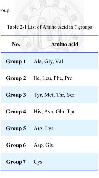
The 20 amino acids could be clustered into seven groups based on the dipoles and volumes of the side chains [13]. Amino acids within the same group likely involve synonymous mutations because of their similar characteristics. Table 2-1 enumerates amino acids in each group.
Table 2-1 List of Amino Acid in 7 groups
No. Amino acid
Group 1
Ala, Gly,ValGroup 2
Ile, Leu, Phe, ProGroup 3
Tyr, Met, Thr, SerGroup 4
His, Asn, Gln, TprGroup 5
Arg, LysGroup 6
Asp, GluGroup 7
Cys11
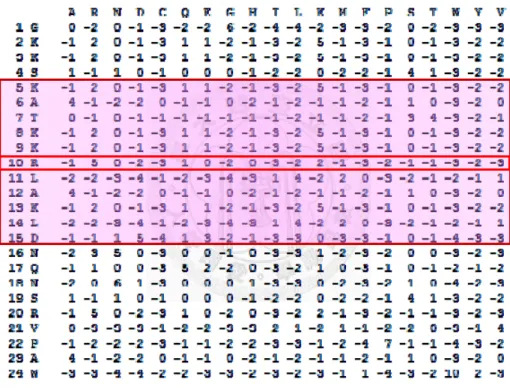
2-3 Position-Specific Scoring Matrix
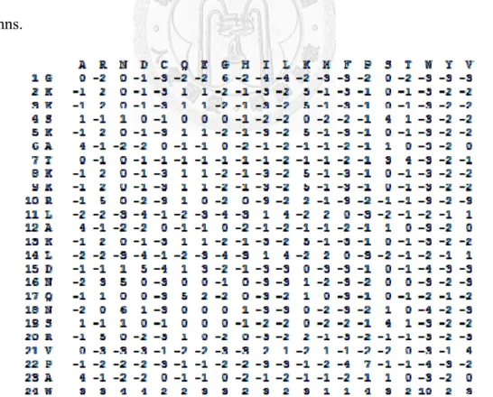
Position-Specific Scoring Matrix (PSSM) can be generated by PSI BLAST [14] by searching against National Center for Biotechnology Information (NCBI) non-redundant (nr) database. A protein sequence in FASTA format is calculated by position-specific scores for each residue independently in the alignment. The score in PSSM is the sum of log-likelihoods under a product-multinomial distribution. Highly conserved residues receive high scores and weakly conserved residues receive low scores. Figure 2-4 depicts the content of PSSM; the query sequences are shown in rows and the types of amino acids comprised of log-likelihoods for 20 amino acids are shown in columns.
Figure 2-4 Part of PDB ID: 1JJ2_1 PSSM
12
2-4 Secondary Structure Information
Protein secondary structure is the general three-dimensional form of local sequence segments. The most common secondary structures are helices and sheets. Each of these two secondary structure elements has a regular geometry, namely stabile hydrogen bonding patterns. The coil is not a bona fide secondary structure, but is the class of conformations that indicates an absence of regular secondary structure.
We obtain protein secondary structures information (SS) by PSIPRED Protein Structure Prediction Server developed by Bryson et al. [15]. The server predicts secondary structures based on amino acid evolutionary information that is PSSM in our thesis.
2-5 Classifier - Support Vector Machines
Support vector machine (SVM) is a powerful machine-learning algorithm developed from statistical learning theory which is based on structural risk minimization proposed by Vladimir Vapnik [8]. Nowadays, SVM is one of the most popular solutions for classification, regression, and novelty detection. Briefly speaking, a SVM constructs a hyper-plane in multi-dimensional space that optimally separates input data into two categories. In the following section, we illustrate the framework of SVM.
13
To begin with, the given data in the multi-dimensional space consist of predictor variables. The predictor variables are called attributes. A transformed attribute that is
used to define the hyper-plane is called a feature. A set of n points of data is in the form:
n
i i ,
,label d x i ,label i x i Dataset
1 1 0
∈
∈
(2-1)
A set of features that describes one case (i.e., a row of predictor values) is called a vector. So the goal of SVM modeling is to find the optimal decision boundary (called hyper-plane) that separates clusters of vectors in such a way that cases with one category of the target variable are on one side of the plane and cases with the other category are on the other side of the plane. The vectors near the hyper-plane are the support vectors that construct the hyper-plane.
We discuss SVMs by a linear separable case. The linear model can be presented in the form:
b b
x
y
( )W
x
W
Tx
(2-2) where (.) means dot product of the W vector and data x, b is a bias parameter.As illustrated in Figure 2-5, the margin is defined as the perpendicular distance between hyper-plane and the closest data points. Maximizing the margin leads to a particular choice of hyper-plane which is in the form:
0 )
(
x
b
y W
Tx
(2-3)14
The two dashed lines in the figure are support hyper-plane, and each satisfied the form respectively:
1 )
(
x
b
y W
Tx
(2-4)1 )
(
x
b
y W
Tx
(2-5)If a data point in the space satisfied the inequality 2-6, this data would be classified as square-shaped points; or, if a data point satisfied the inequality 2-7, it would be denoted the circular points.
1 )
(
x
b
y W
Tx
(2-6)1 )
(
x
b
y W
Tx
(2-7)Figure 2-5 Hyper-plane of SVM
1 )
(
x
b
y W
Tx
b X
Y
margin
1 )
(
x
b
y W
Tx
0 )
( x b
y W
Tx
15
The two inequalities above can be rewritten as:
1 )
(
x b
labeli WT i for all 1in (2-8)
Under the constraint, the hyper-plane therefore has independent data points instead of support vectors. The intuition behind the result is that the decision boundary is increasing dominant by nearby data points relative to the distant ones.
By far, we discussed the condition in two-dimension. In the following, we further apply these formulas to the multi-dimensional problems. We could obtain the distance of a point x to the hyper-plane:
W Wxb
Distance
(2-9)
If we calculate the distance between support hyper-plane and hyper-plane,
W
Tx
b1, than we haveW W
1 1
Distance
b b (2-10)
Thus, the maximum margin solution is found by solving the sum of the two support hyper-planes to the hyper-plane
W
2 that is in the form Find w and b, maximizeW
2 , or minimize 2W
WT (2-11)
It seems that the bias parameter b has disappeared from the optimization. However, it is determined implicitly via the constraints, since this requires that changes to W
be compensated by changes to b.
16
Since the input data might have various distributions in feature space, the linear model might not be suitable for the input data in reality. A kernel technique is developed to map the nonlinear input spaces to linear ones. We can apply Lagrange number α to vector w and rewrite formula (2-8) as:
1 ) (
labeli
j i T j
j
x x b
for all 1in (2-12), where xj is the support vectors.
The kernel function is given by the relation )
( ) ( ) ,
(
x
jx
ix
j Tx
iK
(2-13), where (x) is a space mapping function.
The concept of the kernel formula allows us to build extensions of many well-known algorithms. The common kernel functions are listed below.
Radial basis function: ( , ) exp( 2 )
2
i j i
j
x x x
x
K
Linear function:
K
(x
j,x
i)x
jT x
iPolynomial function:
K
(x
j,x
i)(x
jTx
ib
)DegreeSigmoid function: K(xj,xi)tanh((xjxi)b)
In the general case, we have to consider another problem: data overlapping. We might prefer a solution that better separates the bulk of the data while ignore a few
17
weird noises. In 1995, Corinna Cortes and Vladimir Vapnik proposed soft margin method that allows for mislabeled examples [16]. The previous discussion is based on a hard margin concept that no data exists between two support hyper-planes. On the contrary, the soft margin method introduces a slack variable, ξ, which measures the degree of misclassification of the data x. Moreover, the cost value, C, is a regularization parameter that controls the trade-off between maximizing the margin and minimizing the training error. A small cost value tends to emphasize the margin while ignoring the outliers in the training data, while a large cost value may tend to over-fit the training data. If the penalty function is linear, the optimization problem can be written as:
Minimize:
i
C i 2
2 1 W
Subject to: labeli(
j
jx
Tjx
ib
)1
i (2-14) for all 1in,
i 0This thesis utilized LIBSVM, developed by Chang et al. [17] The LIBSVM package provides classification model construction, regression, multi-class SVM, etc.
With a user-friendly interface and adjustable parameter settings, LIBSVM has been used by many researches in recent years. We choose the Radial basis kernel to implement our predictor.
18
2-6 WildSpan
As we mention, we attempt to extract information only from amino acid sequences.
Mining subsequence that frequently occurs among a set of training sequence, we may obtain information of function annotation, the functional sites, and RNA-protein interaction sites.
WildSpan (http://biominer.bime.ntu.edu.tw/wildspan/) [18] has been embedded in many applications to discover functional signatures and diagnostic patterns of proteins directly from a set of unaligned protein sequences. Therefore, we apply WildSpan to discover conserved residues as RNA-binding residues in a protein sequence to improve prediction performance. For protein-based mining, the authors suggested at most 150 unique homologous proteins with sequence identity ranged from 30% to 90% are required by searching against Swiss-Prot sequence database with PSI-BLAST (blastpgp –j 6). WildSpan cannot generate any patterns in the case of not enough homologous proteins selected from Swiss-Prot protein sequence database or too similar homologous proteins.
2-7 Related Works
Due to the importance of RNA-protein interaction, there are many related studies in the last decade. In 2004, one of the earliest attempts on prediction of RNA-binding sites is Jeong et al. [19] using an artificial neural network (ANN) based on amino acid
19
sequence and secondary structure information in sliding windows. They achieved a maximum Matthew's correlation coefficient (MCC) of 0.294 with five-fold cross-validation by residues. Jeong and Miyano [20] then endeavored to improve the RNA interacting residues prediction based on evolutionary information from the PSSM and achieved MCC, overall accuracy, specificity, and sensitivity of 0.39, 80.20%, 91.04%, and 43.40%, respectively. They established a dataset containing 86 protein chains that has been used most frequently in the studies afterwards. Furthermore, amino acid evolutionary information from the PSSM plays a crucial role and has widely usage.
Scientists have been seeking to find other critical features to improve the performance of their predictors. In 2006, Wang and Brown [21] put forward another method utilizing SVM with side chain pKa, hydrophobicity index and molecular mass of amino acids on 107 protein chains within 25% sequence identities and achieved a maximum accuracy of 69.32% with 66.28% sensitivity. Additionally, they provided a web server predicting both DNA and RNA protein binding sites called BindN [22]. Kim
et al. [23] studied the propensities of individual amino acids and amino acid pairs in
RNA-protein interfaces on the previous 86 protein chains dataset by Jeong et al. [19].
They reported 50% sensitivity and 57% specificity for a method that combined doublet propensities and evolutionary information.
20
As time goes by, the number of known RBPs has rose up to a considerable degree.
Terribilini et al. [24] developed a Naive Bayes Classifier on a larger dataset on PSSM, and achieved maximum MCC of 0.35 in 2007. Tong et al. [25] applied SVM on the same dataset and features as Terribilini did, and obtained a higher MCC 0.365. Wang et
al. [26] reported MCC 0f 0.457 and accuracy of 87.4% by using PSSM, observed
secondary structure information and solvent accessibility information on SVM. In 2008, Kumar et al. [27] utilized a SVM with a second order polynomial kernel and PSSM as input features on 86 protein chains, achieving an MCC of 0.45 (specificity: 89.6%, sensitivity: 53.0%). Cheng et al. [5] encoded PSSM into a new smooth PSSM on SVM classifier, performed a MCC up to 0.68 with five-fold cross-validation on residue-level on 86 protein chains. A high prediction accuracy with a MCC of 0.50 with five-fold cross-validation on residue-level has been reported by Spriggs et al. [28] utilized SVM to analyze input features such as sequence profiles, interface propensities, accessibility and hydrophobicity on only 81 protein chains. Maetschke et al. [29] examined many structural and topological information on both SVM and Naive Bayes Classifier, including constructing graph-theoretical and geometrical sliding windows on 144 protein chains, and reported MCC 0.39 (specificity: 82.0%, sensitivity: 66.8%). All the related works are summarized in Table 2-2.
21
Table 2-2 List of previous RNA-binding prediction works
Authors Methods feature Performance
Jeong et al.[19] Artificial Neural
Network AA sequence and SS MCC 0.29
Jeong and Miyano [20]
Artificial Neural
Network PSSM MCC 0.39
Wang and
Brown [21] SVM
side chain pKa, hydrophobicity index and
molecular mass of AA
69% accuracy and 66% sensitivity
Kim et al.[23] Scoring Function doublet propensities and evolutionary information
50% sensitivity and 57%
specificity Terribilini et al.
[24] Naive Bayes Classifier PSSM MCC 0.35
Tong et al.[25] SVM PSSM MCC 0.37
Wang et al. [26] SVM PSSM, SS and solvent
accessibility information MCC 0.46 Kumer et al.
[27] SVM PSSM and interface
propensities MCC 0.45
Cheng et al. [5] SVM smooth-PSSM MCC 0.68
Spriggs et al.
[28] SVM
PSSM, interface propensities, accessibility
and hydrophobicity
MCC 0.50
Maetschke et al.
[29] SVM
graph-theoretical sliding window PSSM with structural and topological
information
MCC 0.39
Some of the previous studies reported acceptable results of macromolecular sequence data on k-fold cross validation on window-base data splitting which is residue-level cross validation. In spite of that, Caragea et al. [7] pointed out the problems of accessing the performance of classifiers on imbalance data like macromolecular sequence dataset. In comparison of window-based k-fold cross
22
validation and sequence-based k-fold cross validation, window-based cross validation can yield overly optimistic estimates of the performance of classifier relative to the estimates obtained using sequence-based cross validation. This kind of data division has homologous issue biologically that might occur overlapping between these data subsets.
As Table 2-2 shows, SVM has been adopted as a core classifier due to its low bias, high customizability and better performance. Therefore, we choose SVM as one of the core classifiers in this paper. Furthermore, SVM-based single predictors have limited improvement [28]; therefore, we propose a hybrid method named “ProteRNA”.
23
Chapter 3 Method
3-1 Problem Definition
We aim to provide a useful RBP binding site predictor that can assist biologists to have clues on site-directed mutagenesis in wet-lab experiments. With protein sequence information only, we predict the binding residues and output binary label.
The definition of protein-RNA interaction residues is based on molecular distance which is a good indication for existence of intermolecular forces. An amino acid residue was designated as a binding site if the side chain or backbone atoms of the residue fell within a cutoff distance from any atoms of the RNA partner molecule in the complex.
All the other residues were regarded as non-binding sites.
3-2 Data Set
We adopt two training sets and one testing set to perform the experiment.
i. RNA Binding Protein Chain 86 (RBPC86)
As mentioned in the related work, RBPC86 is the most common dataset in the field of RNA-Protein interaction sites prediction. The RBPC86 data set consists of 86 protein chains extracted from RNA-protein complexes with X-ray crystallography resolution better than 3.0 Å in PDB.
This dataset first defined by Jeong and his colleagues [19, 20] as a distance cutoff 6.0 Å to include a wide range of protein-RNA interactions, and the homology is 70%
24
sequence identity over 90% overlap on both sequences and BLASTClust [30]. RBPC86 then used by Kumar et al. [27], and adapted by Cheng et al. [5] as well as Spriggs et al.
[28]. We utilized the Cheng et al. [5] version which has removed non-RBP chains. The resultant data set contains 4,568 RNA interacting residues and 15,503 non-interacting residues, in total of 20,071 residues.
ii. RBPC147
Another training dataset of protein–RNA interactions is RBPC147 extracted from structures of known protein–RNA complexes in the PDB solved by X-ray crystallography resolution better than 3.5 Å. Proteins with larger than 30% sequence identity were removed using PISCES [31].
Terribilini et al. [32] introduced RBPC147 in the RNABindR web-based server. In addition, Tong et al. [25] used RBPC147 as a benchmark dataset. Based on the cut-off distance of 5.0 Å, a total of 32,324 amino acids are included in RBPC 147, which contains 6,157 RNA-binding residues and 26,167 non-binding residues.
iii. RBPC33
An independent testing dataset of protein–RNA interactions is RBPC33 extracted from structures of known protein–RNA complexes that were added after January 2006.
RBPC33 contains chains longer than 40 residues. We performed a redundancy reduction on BLASTClust [30] to ensure that none of the chains showed a sequence
25
similarity of more than 30% within the dataset and to the previous RBPC86 and RBPC147 dataset. A distance cutoff of 5.0 Å was used to annotate interface residues.
RBPC33 is a testing set modified from 36 binding protein chains which were used by Maetschke et al. [29] in 2009.
3-3 Performance Measure
To benchmark our performance and compare with the other studies, we calculate the following measurements:
Recall FN
TP
= TP y
Sensitivit
,
FP TN
= TN y Specificit
,
FP TP
= TP Precision
,
FN FP TN TP
TN
= TP Accuracy
,
FN) (TN FP) (TN FN) (TP ) FP TP (
FN FP TN
= TP
MCC
,
F-score
Recall Precision
Recall Precision
2
,
where TP is the number of true positives, FP is the number of false positives, TN is the number of true negatives and FN is the number of false negatives. An MCC of +1 reaches its best correlation between the observed and the predicted classes of the samples, and a MCC of −1 is perfect anti-correlation; whereas a MCC of zero denotes
26
no correlation at all. F-score (also called F-measure) is a harmonic mean of precision and recall, where 1 denotes perfect results and 0 denotes the worst [33].
In this study, we use two cross-validation ways to assess the performance of the SVM models. One is leave-one-out cross-validation, using a single chain from the RBPC86 as the validation data and the rest of chains as the training data. The cross-validation process is repeated 86 times. The other way is by using 5-fold cross-validation on RBPC147 due to the data over-fitting and the time-consuming problem; we use 5-fold cross-validation on both RBPC86 and RBPC147. RBPC86 and RBPC147 are randomly split into 5 non-overlapping subsets on protein-chain level to avoid homological issue. One subset is the validation data, and the remaining subsets are the training set. Then repeat 5 times to generate the performance of our predictor.
3-4 Feature Selection
To obtain the best performance of prediction, we explore distinct features and PSSM schema to apply to our experiments.
i. PSSM
PSSM encoded from PSI BLAST is composed of log-likelihoods for 20 amino acids for individual query residues.
27
ii. PSSM in 7 groups
PSSM encoded according to amino acid properties of 7 groups shown in Table 2-1 in Chapter 2. After the PSSM turn into a 7-column matrix, we encoded to a sequence patch using sliding window technique.
iii. PSSM added secondary structure information (SS)
The PSIPRED outputs consist of three probability values represented for helix, sheet and coil respectively, for instance (H, E, C) = (0.75, 0.25, 0.25). We add three features to a normalized PSSM features then do the sliding window, that is to say, the added secondary structure information is not normalized.
iv. PSSM added interface propensities
The interface propensities calculate the proportion of the interface to surface of a given residue in RBPs.
k k
S k S
k I k I
k
N N
N N
propensity
Interface (3-1)
where N is the number of interface residues of certain type of amino acid k, Ik
k IN the total number of interface residues, k N is the number of surface residues Sk of type k, and
kS
N are the number of surface. We adopt a new interface propensity k
calculated by Laura Pe´rez-Cano et al. [34] The interface propensities are normalized in linear model due to its range from 0 to1.
28
v. PSSM added Electrostatics propensities
PSSM is added one column of electrostatics propensities based on amino acid attributes, ascertained by Fauchere, J.L. et al. [35] In our schema, 0 means negative charge, 0.5 represents neural and 1 means positive charge.
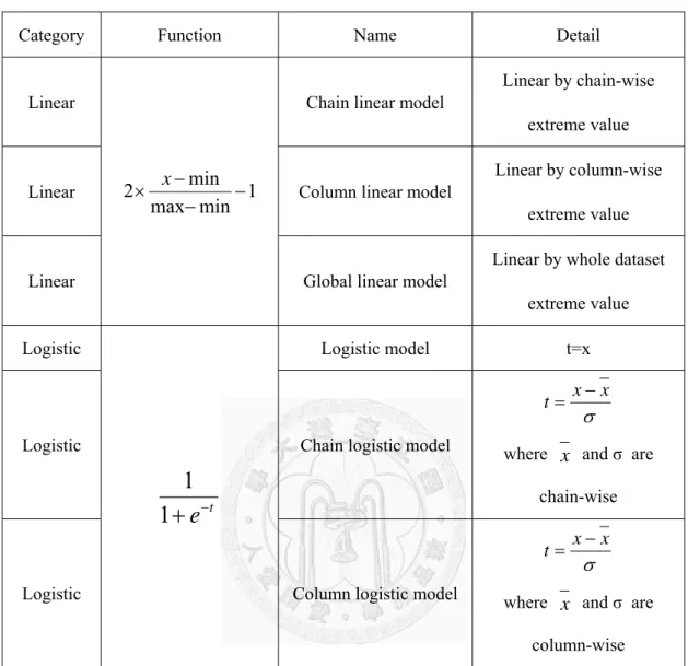
3-5 Normalization
Normalization is a crucial topic in the process of handling data. The most important purpose of normalization is to avoid attributes in greater numeric ranges dominating those in smaller numeric ranges. On the other hand, it is utilized to avoid numerical difficulties or even computation crashes during the calculation when dimension grows large. On a common basis, researchers normalize each attribute of the data instance to the range [0,1] or [-1,1].
Figure 3-1 Linear model (in dashed), Logistic model (in blue)
29
We adopt two major model of normalization: linear model and logistic model. By instinct, the linear model is scaling to proportion of maximum and minimum. For scaling to [-1,1], the linear model is
min 1 max 2 min model
Linear
x
, (3-2)where min stands for minimum and max for maximum.
For linearly separable data, over-fitting might occur, since the extreme value of maximums or minimums affect the scaling curve. We can use local maximum and local minimum of each protein chain or normalize input value by each amino acid in column to resolve such situations.
In addition, another solution is adapting logistic model, the so called sigmoid model [36]. To scale data attributes to [0,1], the logistic model uses the following equation:
e
x 1 model 1
Logistic (3-3)
Since we try to avoid data bias, we propose a modified version of the logistic model that shifts the curve according to their mean and variance.
e
t 1 model 1
Logistic ,
x
t x (3-4)
where x is the mean value and σ is the standard deviation.
Table 3-1 is the detailed normalization functions categorized in linear or logistic models discussed in this thesis.
30
Table 3-1 List of normalization functions
Category Function Name Detail
Linear
min 1 max
2 min
x
Chain linear model
Linear by chain-wise extreme value
Linear Column linear model
Linear by column-wise extreme value
Linear Global linear model
Linear by whole dataset extreme value Logistic
e
t1 1
Logistic model t=x
Logistic Chain logistic model
x t x
where
x
and σ are chain-wiseLogistic Column logistic model
x t x
where
x
and σ are column-wiseThe results of distinct normalization ways are reported in 4-1 . We find out that Logistic model outperform the others methods; hence, Logistic model are adopted in the following experiment.
3-6 Single Predictor Model
The performance of the SVM classifier depends on the combination of several parameters. In general, our experiment involves two groups of parameters: parameters relative to input featured PSSM and SVM classifier adjustment.
31
The first one is the sliding window size of featured PSSM. PSSM generates evolutional information of individual residue and added amino acid properties. Since a residue cannot act as a lonely wolf in biochemical process, we cluster neighboring residues to a central residue and construct sequential patches. By using sliding windows, the sequence properties were integrated into a feature vector covering the whole subsequence and all the information is used to describe the center residue.
Figure 3-2 Sliding window framework
For the SVM classifier, we take two parameters into account. The first one is cost value C, and the other is γ gamma value in the radial basis function. The cost value C is a regularization parameter that controls the trade-off between maximizing the margin and minimizing the training error, while the gamma value γ regulates the amplitude of the kernel function to dominate the generalization ability of SVM.
32
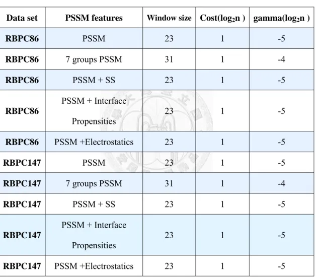
We test a wide range of window sizes according to the featured type of PSSM.
Since 7-group PSSM extracts features vector out of 7 columns, we obtain a larger window size of 31 to gather enough information. The others window sizes of featured PSSM are about 23, which is around the domain size in RBPs.
Table 3-2 List of optimal parameters of single predictors
Data set PSSM features
Window sizeCost(log
2n ) gamma(log
2n )
RBPC86
PSSM 23 1 -5RBPC86
7 groups PSSM 31 1 -4RBPC86
PSSM + SS 23 1 -5RBPC86
PSSM + Interface
Propensities 23 1 -5
RBPC86
PSSM +Electrostatics 23 1 -5RBPC147
PSSM 23 1 -5RBPC147
7 groups PSSM 31 1 -4RBPC147
PSSM + SS 23 1 -5RBPC147
PSSM + Interface
Propensities 23 1 -5
RBPC147
PSSM +Electrostatics 23 1 -5The corresponding results are listed and discussed in Section 4-2 . Since the improvements of the single predictors are limited, we propose a hybrid model.
33
3-7 Hybrid Model
Besides diverse PSSM schemas and features as single predictor, we devote to seek models that predict more positive values which mean RBP binding sites. Since the protein functional signatures are strongly related to the conservation domains, we consider RNA-protein interaction as a kind of protein function and utilize WildSpan to find conservation domains. We combine SVM-based single predictors which combined PSSM and secondary structure information together with WildSpan to construct a new model.
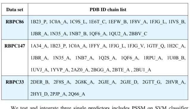
We applied the default parameter setting to obtain patterns by WildSpan. As the authors recommend, we input our query to search against Swiss-Prot database [3] with PSI-BLAST (blastpgp –j 6) and obtain maximum 150 unique target sequences. These target sequences share 30% ~ 90% sequence identity with the query sequence, since we would like to find remote homologous domains and to remove the similar protein sequence. Then we utilize WildSpan to obtain the top-one conservation pattern as the binding residues. Since WildSpan cannot generate patterns under certain conditions, we have several chains without WildSpan patterns. There are 14 chains out of RBPC86, 21 chains out of RBPC147, and 11 chains out of RBPC33. The detailed list of protein chains with no WildSpan patterns are enumerated in Table 3-3.
34
Table 3-3 List of protein chains with no WildSpan patterns
Data set PDB ID chain list
RBPC86 1B23_P, 1C0A_A, 1C9S_L, 1E6T_C, 1EFW_B, 1F8V_A, 1FJG_L, 1IVS_B, 1JBR_A, 1N35_A, 1NB7_B, 1QF6_A, 1QU2_A, 2BBV_C
RBPC147 1A34_A, 1B23_P, 1C0A_A, 1FFY_A, 1FJG_L, 1FJG_V, 1GTF_Q, 1H2C_A, 1JBR_A, 1N35_A, 1NB7_A, 1Q2S_A, 1QF6_A, 1RPU_A, 1U0B_B, 1UVJ_A, 1YVP_A, 2AZ0_A, 2BGG_A, 2BTE_A , 2BU1_A
RBPC33 2DER_B, 2F8S_A, 2G8K_A, 2GJE_A, 2GJE_D, 2GTT_G, 2HVR_A, 2HYI_D, 2PJP_A, 2Q66_A
We test and integrate three single predictors includes PSSM on SVM classifier, PSSM added secondary structure information on SVM classifier as well as pattern information by WildSpan. The new model incorporates all the positive sites that identified by single predictors. We name this Protein-RNA sites prediction method ProteRNA.
3-8 System Architecture
Our experimental method has two main parts as Figure 3-3. Firstly, sequence queries are prepared in FASTA format. Secondly, we input sequence queries to runs on SVM to get a prediction model. Finally, WildSpan provides the conservation information and outputs the second model. After we combine the entire prediction model, the result is done.
35
Figure 3-3 Overall framework flowchart
The detailed experiment steps are shown in Figure 3-4 and Figure 3-5. In Figure 3-4, we depict SVM part. Firstly, sequence queries are encoded to PSSM by PSI BLAST and normalized by logistic function. Secondly, we prepare the PSSM by adding secondary structure information provided by PSIPRED. The PSSM with secondary structure information combined and do the sliding window to be the training data. The training data runs on SVM to get a prediction model.
The WildSpan part is shown in Figure 3-5. We input our query to search against Swiss-Prot database [3] and obtain maximum 150 unique target sequences that share 30% ~ 90% sequence identity with the query sequence. Then we input these sequences to WildSpan and obtain the top-one conservation pattern as the binding residues. Since
36
WildSpan cannot generate patterns under certain conditions, we have several chains without WildSpan patterns as enumerated in Table 3-3.
Figure 3-4 Secondary structure information prediction flowchart
37
Figure 3-5 WildSpan prediction flowchart
38
Chapter 4 Results and Discussion
4-1 Distinct Normalization Results
Data normalization is the very first step to handle data instances, namely, sequence evolutional information in our study. We use two different categories which are linear normalization and logistic normalization. Each normalization method in the same category shares the same features with minor modifications on the equation.
We take RBPC86 to examine the performance of each normalization functions.
Table 4-1shows the results of 5-fold cross-validation of RBPC86 using PSSM.
Table 4-1 Results of different normalization functions (order by MCC)
Name Sensitivity Specificity Precision Accuracy MCC F-score
Logisticmodel
45.73% 95.68% 75.74% 84.31% 0.5043 0.5702
Chain linear model
43.18% 95.59% 74.25% 83.66% 0.4796 0.5460
Chain logistic model
43.04% 95.17% 72.43% 83.31% 0.4685 0.5400
Column logistic model
40.79% 95.72% 73.73% 83.22% 0.4615 0.5253
Column linear model
39.61% 95.97% 74.34% 83.14% 0.4570 0.5168
Global linear model
27.67% 97.89% 79.43% 81.91% 0.3966 0.4104
39
From Table 4-1, we can tell that logistic model achieve the highest accuracy, MCC and F-score of 84.31%, 0.5043, and 0.5702 respectively. There is a gap between logistic model and chain-based linear model of MCC 2.47% and F-score 2.42%. To sum up, logistic models outperform linear models, and chain-based information is better than column-based or amino acid features normalization ways.
4-2 Performance of Single Predictor
We explore different features on a single predictor to gain knowledge from the RNA prediction. The following tables report the results different cross validation ways on each datasets. The top-one accuracy, F-score and MCC are marked in bold.
Table 4-2 Results of single predictor using leave one out cross validation on RBPC86
Name Sensitivity Specificity Precision Accuracy MCC F-score PSSM
45.64% 95.57% 75.22% 84.21% 0.5008 0.56817 groups
PSSM
40.72% 95.78% 73.99% 83.25% 0.4623 0.5253
PSSM + SS
47.15% 95.19% 74.30%84.26% 0.5051 0.5769 PSSM +
Interface Propensities
46.30% 95.41% 74.81% 84.23% 0.5027 0.5720
PSSM +Electrostat
ics
43.89% 96.03% 76.53% 84.17% 0.4969 0.5579
40
Table 4-3 Results of single predictor using five cross validation on RBPC86
Name Sensitivity Specificity Precision Accuracy MCC F-score PSSM
45.73% 95.68% 75.74%84.31% 0.5043 0.5702 7 groups
PSSM
39.44% 95.83% 73.59% 83.00% 0.4519 0.5136
PSSM + SS
44.28% 95.80% 75.67% 84.08% 0.4947 0.5587PSSM +
Interface Propensities
45.91% 95.53% 75.19% 84.24% 0.5023 0.5701
PSSM +Electrostat
ics
42.54% 95.90% 75.37% 83.76% 0.4817 0.5438
The previous tables show the results of RBPC86 with different cross validation procedures in each measurement. They show slightly different in models peak values and performances ranking between models. In leave-one-out cross validation, PSSM added secondary structure information achieve 0.5051 MCC, 0.5769 F-score and 84.26% accuracy, while PSSM only achieve 0.5008 MCC, 0.5681 F-score, and 84.21%
accuracy. On the other hand, in 5 fold cross validation, PSSM added secondary structure information only achieve 0.4947 MCC, 0.5587 F sore, and 84.08% accuracy, whereas PSSM reach 0.5043 MCC, 0.5702 and 84.31% accuracy.
41
Table 4-4 Results of single predictor using five cross validation on RBPC147
Name Sensitivity Specificity Precision Accuracy MCC F-score PSSM
38.60% 96.85% 74.26% 85.76% 0.4661 0.50807 groups
PSSM
33.07% 97.13% 73.05% 84.93% 0.4224 0.4553
PSSM + SS
38.85% 97.01% 75.35%85.93% 0.4732 0.5127 PSSM +
Interface Propensities
37.71% 97.03% 74.90% 85.73% 0.4632 0.5016
PSSM +Electrostat
ics
38.04% 96.98% 74.77% 85.75% 0.4648 0.5042
Table 4-4 shows the performance of RBPC147 in 5 fold cross validation. The peak values are PSSM added secondary structure information of MCC, F-score and accuracy of 0.4732, 0.5127 and 85.93%; on the contrary, the bottom values are PSSM in 7 groups of 0.4224 MCC, 0.4553 F-score, and 33.07% accuracy. The plan PSSM delivers 0.4661 MCC, 0.5080 F-score, and 85.76% accuracy.
42
Figure 4-1 Performances of single predictors in line chart in F-score
As Figure 4-1 illustrates, RBPC86 using leave-one-out cross validation delivers better overall performance on F-score than the others. Since some studies shows leave-one-out cross validation may occur over-fitting, we conclude that RBPC86 performs on F-score around 0.57 are the same level that correspond to previous study.
Due to the data imbalance problem, that is to say the negative to positive ratio of RBPC147 is 5.25:1 which is higher than that of RBPC86 (3.27:1), the F-score of RBPC147 in 5 fold cross validation is lower than that of RBPC86 by about 6 percents.
On the contrary, since the proportion of true negative value is higher in RBPC147 results, accuracy of RBPC147 is higher than RBPC86 by around 2 percents.
43
To sum up, not all of the proposed features have significant improvement. Besides the 7 group PSSM schema, the added feature might have a chance to elevate the performance by a limited degree. Yet the true positive number must be raised up a certain level to be useful to biologists on the site-direct mutagenesis. This conclusion agrees the previous study by Spriggs et al. that they stated the overlap between their single predictors is high and inferred the single predictors have limited improvement.
[17] As a result, we propose hybrid model.
4-3 Performance of Hybrid Model
We select top-two single predictors o integrate with data from Wildspan . The following tables report the results different cross validation ways on each datasets with standard deviation. The top-one accuracy, F-score and MCC are marked in bold.
Table 4-5 Results of hybrid model using leave-one-out cross validation on RBPC86
Name Sensitivity Specificity Precision Accuracy MCC F-score
WildSpan(1)
8.36% 97.28% 47.51% 77.04% 0.1206 0.1422PSSM(2)
45.64% 95.57% 75.22% 84.21% 0.5008 0.5681(1)+(2)
49.65% 93.18% 68.19% 83.27% 0.4829 0.5746 PSSM+SS(3) 47.15% 95.19% 74.30%84.26% 0.5051
0.5769(1)+(3)
50.88% 92.80% 67.54% 83.25% 0.4858 0.5804(1)+(2)+(3)
53.88% 91.97% 66.41% 83.30% 0.49540.5949
44
The highest F-score is 0.5949 of the model combine PSSM, PSSM+SS, and WildSpan in leave-one-out cross validation. The F-score of PSSM is improved from 0.5681 to 0.5949 for more than 2 percents, mainly because sensitivity is improved for 8 percents. We can see from the table that merge WildSpan information and each single predictor together improved less than one percent. However, the highest accuracy and MCC are still located in PSSM+SS.
Table 4-6 Results of hybrid model using five-fold cross validation on RBPC86
Name Sensitivity Specificity Precision Accuracy MCC F-score WildSpan(1)
8.36% 97.28% 47.51% 77.04% 0.1206 0.1422PSSM(2)
45.73% 95.68% 75.74%84.31% 0.5043
0.5702std
0.36% 0.06% 0.35% 0.11% 0.40% 0.37%(1)+(2)
49.64% 93.31% 68.60% 83.37% 0.4855 0.5760std
0.32% 0.06% 0.29% 0.11% 0.36% 0.31%PSSM+SS(3) 44.28% 95.80% 75.67% 84.08% 0.4947 0.5587
std
0.47% 0.21% 0.85% 0.14% 0.45% 0.35%(1)+(3)
48.09% 93.55% 68.71% 83.20% 0.4770 0.5658std
0.72% 0.14% 0.21% 0.07% 0.36% 0.46%(1)+(2)+(3)
53.08% 92.46% 67.48% 83.50% 0.49810.5942
std
0.31% 0.05% 0.21% 0.08% 0.29% 0.26%45
The integrated model of PSSM, PSSM added secondary structure information, and conservation information from WildSpan delivers 0.5942 F-score in 5 fold cross validation. Which is also improved more than 2 percents of F-score, because of a 7 percent sensitivity improvement. On the contrary, the peak value of accuracy and MCC are the original PSSM.
Table 4-7 Results of hybrid model using five fold cross validation on RBPC147
Name Sensitivity Specificity Precision Accuracy MCC F-score WildSpan(1)
14.28% 94.68% 43.60% 76.69% 0.1432 0.2151PSSM(2)
38.60% 96.85% 74.26% 85.76% 0.4661 0.5080std
0.44% 0.08% 0.38% 0.05% 0.27% 0.35%(1)+(2)
44.83% 93.44% 61.66% 84.18% 0.4351 0.5192std
0.37% 0.08% 0.16% 0.04% 0.19% 0.23%PSSM+SS(3) 38.85% 97.01% 75.35% 85.93% 0.4732 0.5127
std
0.46% 0.09% 0.48% 0.08% 0.36% 0.40%(1)+(3)
45.04% 93.64% 62.48% 84.38% 0.4413 0.5235std
0.37% 0.09% 0.25% 0.06% 0.27% 0.27%(1)+(2)+(3)
47.75% 92.86% 61.15% 84.27% 0.4482 0.5362std
0.30% 0.08% 0.21% 0.05% 0.20% 0.20%46
For RBPC147, the integrated model of PSSM, PSSM+SS, and WildSpan delivers noticeably higher F-score of 0.5942 in 5 fold cross validation, which is improved more than 3.5 percents of PSSM F-score, because of almost 10 percent sensitivity improvement. By contrast, the peak value of accuracy and MCC are the PSSM added secondary structure information.
Figure 4-2 Performances of hybrid models in line chart in F-score
From Figure 4-2, we can tell that the combined models outperform the original single predictors. We notice that even though logically PSSM added secondary structure information predictor should include the information form plain PSSM predictor, there are still slightly different between the two models. Since the best F-score are obtained
47
from the three single predictors integrated together. Therefore we obtain the three predictor combined results as our final model.
Previous research on RNA-binding domains figured out that RNA binding proteins are composed of multiple repeated blocks of RNA-binding domains to provide diverse functions. Therefore, conserved residues in the same RNA-binding domain from different RNA-binding proteins would not always involve interacting with RNA at the same location. Furthermore, while combining prediction results predicted by single predictors and WildSpan, WildSpan detected additional RNA-binding residues by providing domain-wise conservation information that single predictors did not predict.
The greatest improvement is on RBPC147, since RBPC147 is a larger dataset with high proportion of hard-predicted tRNA. It shows that our method provide more positive
values which might help biologists do in vitro experiments.
4-4 Comparison with Other Approaches
We use RBPC86 in order to compare with the previous studies on the same basis.
The followings are the previous work using RBPC86. The work Jeong2004 is using an artificial neural network by Jeong et al. [19]. Then Jeong improved his work using PSSM, which is called Jeong2006. PPRint is a web service developed by Kumar et al.
[27] in 2008.
48
Table 4-8 Performance comparison on RBPC86 order by F-score
Name Sensitivity Specificity Precision Accuracy MCC F-score ProteRNA
53.08% 92.46% 67.48%83.50% 49.80% 0.5942 PPRint
53.05% 89.55% 60.20% 81.16% 45.00% 0.5642Jeong2006
43.40% 91.00% 58.79% 80.20% 39.00% 0.4994RNABindR
43.00% - 47.00% 76.60% 30.00% 0.4491Jeong2004
40.30% - 46.70% 77.50% 29.40% 0.4326 As Table 4-8 shows, our performance delivers accuracy, MCC, and F-score of 83.50%, 49.8%, and 0.5942, respectively that outperforms all the previously published methods on RBPC86.The RBPC147 dataset is the latest and largest dataset used in RBP sites prediction.
We only find two previous studies report their performance: RNABindR (Terribilini et
al., 2007) and RISP (Tong et al., 2007).
Table 4-9 Performance comparison on RBPC147 order by MCC
Name Sensitivity Specificity MCC ProteRNA
47.75% 92.86%44.8%
RISP
66.4% 75.8% 36.5%RNABindR
33.0% 95.0% 36.0%49
Since the RISP reported only these three measurements, we compare our performance on MCC. Our methods ProteRNA reports MCC of 44.8%, which improves for 8.3% than RISP. We could conclude that ProteRNA achieve a better performance than the previous works on both PBPC86 and PBPC147.
4-5 Independent Test and Comparison with Other Approaches
We use RBPC33 as a testing set to verify our performance and the others web servers. Since cross validation way does not affect independent test, we use RBPC86 and RBPC147 as two training model. For comparison, we use web server BindN, Pprint, PRIP, PiRaNha. Thesepredictions were carried out using defaultparameters settings.
The top-one measure matrixes are marked in bold.
Table 4-10 Independent Test order by F-score
![Figure 1-1 Common RNA-binding protein families [2]](https://thumb-ap.123doks.com/thumbv2/9libinfo/9604633.630790/10.892.204.663.132.757/figure-common-rna-binding-protein-families.webp)
![Figure 2-2 Flow chart of central dogma [10]](https://thumb-ap.123doks.com/thumbv2/9libinfo/9604633.630790/16.892.142.725.600.1045/figure-flow-chart-central-dogma.webp)
![Figure 2-3 Amino acid properties [11]](https://thumb-ap.123doks.com/thumbv2/9libinfo/9604633.630790/17.892.159.713.545.1098/figure-amino-acid-properties.webp)