Labor Market Effects of Outward Direct Investment and Trade: Evidence from Taiwan

Labor Market Effects of Outward Direct Investment and Trade: Evidence from Taiwan

Yen-Chen Chen, Chun-Fang Chiang February 21, 2016

Abstract

In recent decades, Taiwanese investment in China has grown fast and caused concerns of reducing job opportunities in Taiwan. At the same time, net exports from Taiwan to China also has steadily grown.

In this paper, we examine the labor market effects of Taiwan’s outward investment in China and net exports from Taiwan to China between 1998 and 2010. We consider a model in which a multinational firm, when selling its good in China, can choose to export its good to China or produce products in China via outward investments. By applying the theoretical framework on the merged Taiwanese individual-level and industry-level datasets, we found empirical evidence suggesting that outward investment in China has negative effects on wage, al- though skilled workers suffer less. In addition, we discovered that this outward investment increases the unemployment rate of unskilled la- borers while lowering that of skilled laborers. Net exports to China, in contrast, raises unskilled laborer’s wage levels at a higher rate than skilled laborers, thereby contributing to the shrinking of the skill pre- mium. Net exports also decrease the unemployment rate of unskilled laborers at the cost of increasing the unemployment rate for skilled laborers.

1 Introduction

In recent decades, China has expanded fast economic growth and be- came Taiwan’s largest investment destination. Many Taiwanese firms have shifted production outward to reduce the production cost or to be more close to the growing market. The term ‘hollowing-out,’ as often mentioned in the media, suggests a prevalent negative attitude to- wards this trend.¹ While the large-scale outward investment in China might attribute to the wage stagnation phenomenon in Taiwan, in the meantime, net exports from Taiwan to China have been growing. On the one hand, the growing market in China provides an incentive for MNEs to engage in the direct investment in China. On the other hand, China’s growing economy causes a higher demand for interme- diate goods and final goods. In this paper, we investigate labor market effects of both ODI and trade caused by the growing China economy.

Outward direct investment (ODI) and trade are two important factors tied with globalization. How they affect the welfare of work- ers becomes an urgent question as outward investment regulations loosen and trade barriers decline. The standard framework treats ODI as strategy belonging to multinational enterprises’ (MNEs) (La- torre, 2009). Its impact on the domestic labor markets hence may depend on the types of investments. Horizonal investment, for the purpose of producing similar products as in the home country, tends to decrease production and the labor demand in the parent company (Markusen and Maskus, 2001). Vertical investment, meant to save manufacturing costs in certain stages of production, could produce a complementary domestic labor demand (Helpman, 1984). Harri- son and McMillan (2011) distinguished horizontal and vertical ODI using detailed firm-level data, and find that vertical outward invest- ment improves domestic labor- market outcomes, while a horizontal one does not. Because MNEs strategies are not often clearly identi- fied in the data, many researchers distinguishe the types of investment by the destinations of ODI, and find that investing in a country less advanced than home country can substitute for domestic employment (Simpson, 2012; Debaere et al., 2010). In contrast, Castellani et al.

(2008) and Navaretti et al. (2010) have found that investment in coun- tries with cheap labor has no negative effects or a positive effect on employment in developed countries. Becker and Muendler (2008) and Desai et al. (2009) have both concluded that, overall, the prevention of FDI results in higher unemployment and that increased outward investment stimulates domestic employment.

1‘China causes Taiwanese brain drain’ by Financial Times on March 31, 2013.

In the case of Taiwan and China, Tsou et al. (2013) found that workers in firms with higher level of investment in China are more likely to be unemployed, particularly for less-educated workers. Tsaur et al. (2006) found that outward investment is harmful to low-skilled workers’ wage.

The traditional framework to analyze the labor-market effects of trade comes from the Heckscher-Ohlin model and focus on distribu- tional effects. Yet some empirical studies have shown that the labor- market effects of trade liberalization are inconsistent with what the HO model predicts (Harrison et al., 2010). In an environment with a higher openness to trade, the wage gap between skilled and un- skilled workers in developing countries widens instead of narrowing (Goldberg and Pavcnik, 2007; Han et al., 2012). Also contradicting the model, competition from developing countries places no downward pressure on unskilled workers’ wages in developed country such as the US (Edwards and Lawrence, 2010).

From approaches other than the HO model framework, long-term and cross-country surveys such as those of Dutt et al. (2009) and Fel- bermayr et al. (2011) have found that trade openness is negatively re- lated to structural unemployment. Hasan et al. (2012) have also found that workers in industries more open to trade are less likely to be un- employed. However, using China as the source of import competition, Alvarez and Claro (2009) found negative effect on employment growth´ in a developing country. Likewise, Federico (2014) and Mion and Zhu (2013) found negative effects on employment growth for downstream industries, labor-intensive industries and low-tech manufacturing in- dustries in developed countries. Autor et al. (2013) found that workers in regions exposed to higher import competition from China experi- ence wage declines the manufacturing sector. McLaren and Hakobyan (2010) have found that the blue-collar workers in labor-intensive in- dustries suffer from wage losses. Similarly, Ebenstein et al. (2014) have found that workers switching within manufacturing industries experience no wage losses, while workers switching to service sectors do suffer from wage losses.

Though the majority of studies in the literature only focus on one of ODI or trade, the labor-market effects of ODI should be considered alongside trade because ODI activities might affects export activities.

Under horizontal ODI, production originally belonging to the parent company is shifted to foreign affiliates. Therefore, a home country’s exports and ODI are substitutes. Under vertical ODI, exports and ODI are likely complements because intermediate goods are exported from the home country to foreign affiliates. Empirical evidence points out a complementary relationship between ODI and trade, yet Fung

et al. (2013) found them to be substitutive in the case of Taiwan and China. Bergstrand and Egger (2007) have developed a model with three countries, three kinds of factors of production, and three types of firms. In this model they demonstrate how firms involved in importing and exporting, horizontal ODI, and vertical ODI interact and affect return on capital, skilled labor and unskilled labor in each country.

Our approach builds on that of Autor et al. (2013) and extends it by including both ODI and trade. We consider a system of many small open economies, firms of which not only export but also engage in horizontal outward investment in China. When a shock due to a higher demand from China enters the system, the employment in each industry and the wage in the small economy play out in a general equilibrium. The model predicts that the changes of values of ODI and net exports causes the changes in the wage level and employment of the small open economy. We further derive measures for changes brought about by ODI and net exports which can be used to test the model empirically.

Using the trade and ODI data at industry level, and labor force composition of industry data for each county/city, we constrct mea- sures of trade and ODI indexes for each city/county as guided by the model. We then combine them with individual data of wage and em- ployment status for estimations. The OLS estimates might be biased if Taiwaneese economy experienced negative domestic demand shocks that affect labor demand and goods imports simultaneously, or if Tai- waneese economy experienced negative productivity shocks that affect both firms’ investment decisions and workers’ wage level. We employ the IV approach to deal with these problems.

Our results show that for male, increased ODI has the positive effects on skilled labor’s employment. Unskilled labor’s wage and em- ployment are both found to be negatively related with increased ODI.

As to trade, our results indicate that for male, increasing net exports to China raises unskilled labor’s wage level. Trade thus diminishes the relative wage between skilled and unskilled workers. Furthermore, skilled labor’s unemployment increases and unskilled one’s decreases.

1.1 Literature Review

Many studies have examined the effects of either ODI or trade. Re- garding ODI, past research has found no robust evidence for clear labor-market effects. Harrison and McMillan (2011) distinguished horizontal and vertical ODI using detailed firm-level data, and their results largely support the theoretical prediction that vertical outward

investment improves domestic labor- market outcomes, while a hori- zontal one does not. Because MNEs strategies are not often clearly identified in the data, most research distinguishes the effects by the destinations of ODI. Debaere et al. (2010) have found that investing in a country more advanced than the home country has no effects on do- mestic employment but that investing in a country less advanced than home country has negative effects. Simpson (2012) has found that in- vesting in low-wage countries can substitute for domestic employment, especially in low-skill industries. In contrast, Castellani et al. (2008) and Navaretti et al. (2010) have found that investment in countries with cheap labor has no negative effects or a positive effect on em- ployment in developed countries. Becker and Muendler (2008) and Desai et al. (2009) have both concluded that, overall, the prevention of FDI results in higher unemployment and that increased outward in- vestment stimulates domestic employment. In the case of Taiwan and China, Tsou et al. (2013) found that workers in firms with higher level of investment are more likely to be unemployed, particularly for less- educated workers. Tsaur et al. (2006) found that outward investment is harmful to low-skilled workers’ wage.

On the effects of trade, long-term and cross-country surveys such as those of Dutt et al. (2009) and Felbermayr et al. (2011) have found that trade openness is negatively related to structural unemployment.

Hasan et al. (2012) have also found that workers in industries more open to trade are less likely to be unemployed. However, using China as the source of import competition, ´Alvarez and Claro (2009) found negative effect on employment growth in a developing country. Like- wise, Federico (2014) and Mion and Zhu (2013) found negative effects on employment growth for downstream industries, labor-intensive in- dustries and low-tech manufacturing industries in developed countries.

When specifically focusing on the effects developing countries make on developed countries, Autor et al. (2013) found that workers in re- gions exposed to the manufacturing sector experience wage declines.

McLaren and Hakobyan (2010) have found that the blue-collar workers in labor-intensive industries suffer from wage losses. Similarly, Eben- stein et al. (2014) have found that workers switching within manufac- turing industries experience no wage losses, while workers switching to service sectors do suffer from wage losses.

Though the majority of studies in the literature only focus on one of ODI or trade, the labor-market effects of ODI should be considered alongside trade because ODI activities might affects export activities.

Under horizontal ODI, production originally belonging to the parent company is shifted to foreign affiliates. Therefore, a home country’s exports and ODI are substitutes. Under vertical ODI, exports and

ODI are likely complements because intermediate goods are exported from the home country to foreign affiliates. Empirical evidence points out a complementary relationship between ODI and trade, yet Fung et al. (2013) found them to be substitutive in the case of Taiwan and China. Bergstrand and Egger (2007) have developed a model with three countries, three kinds of factors of production, and three types of firms. In this model they demonstrate how firms involved in importing and exporting, horizontal ODI, and vertical ODI interact and affect return on capital, skilled labor and unskilled labor in each country.

2 Background

The economic ties between Taiwan and China grew closely in the 1990s. In 1992, investment in China became legal in Taiwan. The next year, trade with China surpassed that of America. In little more than a decade, China had become the biggest investment destination and the largest trade partner of Taiwan.

Back in 1996, the depreciation of the RMB, cheap labor and cul- tural similarities made China an attractive investment destination for Taiwan. Yet the government’s attitude toward Chinese investment was cautious. Under the ‘patience over haste’ policy, the high-tech and infrastructure industries were restricted from making investments in China, and 50 million dollar ceiling was imposed on every project.

The average investment that year was about 30 million dollars. Since 2002, the investment policy has become increasingly open, relaxing restrictions on high-tech, banking and service industries as well as the investment ceiling.² Figure 1 shows the trend of deflated approved outward investment as recorded by the Investment Commission. In 1993, 1997 and 2002, MNEs that had previously failed to file ODI within the time limit was allowed to refile, thus creating a peak in each of those years. ODI increased by 136% from 1992 to 2010; in the meantime, real GDP grew by 130%. In fact, the amount of ODI could have been larger because much of the ODI going to China go through third parties, such as Hong Kong or the Cayman Islands. For exam- ple, according to Chen (2004), the cumulative approved ODI by 2002 was recorded to be 3.1 billion dollars by the Investment Commission, 3.4 billion dollars by China, and 6 billion dollars by the Central Bank of Taiwan.

The primary source of ODI was from the manufacturing sector, accounting for more than 90% of all ODI before 2002. This percent-

2More details about the policy and restrictions are in Tsou et al. (2013).

age declined to 82% in 2009. With China’s export-promotion policy, many MNEs began receiving orders in Taiwan, producing products in China, and directly exporting them. Among the manufacturing sec- tor, electrical components, computer and optical products have always been the biggest investors. Food and beverage, textiles, and plastic composed a large proportion of investment in earlier times, though now their positions have been replaced by chemical material, metal, non-metal mineral, and machinery. These changes show the process of industry skill-upgrades — a shift from labor-intensive industries to capital-intensive ones.

Trade plays another important role in cross-strait economics. Tai- wan is a country highly dependent on trade. According to TIER (2010), Taiwan’s degree of dependence upon foreign trade, defined as the value of imports and exports relative to the GDP, has risen from 74% in 1990 to 126% in 2010. During the same period, the average degree of dependence upon foreign trade in America was only 20%;

Japan’s was 20%; and South Korea’s was 63%. Among the trade between Taiwan and China, intermediate goods accounts for a large proportion. The percentage of exported intermediates to China has been over 90% since 1992 and has been more than 80% since 1998.

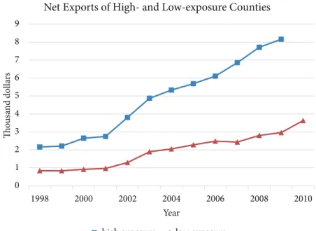
The main export industry is similar to that of the industries for ODI. The electronics industry has become the largest exporter since 1998. Textiles was once the primary export, but today chemical ma- terial, metal, and machinery manufacturing has gradually become the second largest export, falling behind only electronic products. The change in the industry structure of exports is consistent with that of ODI, showing a skill-upgrade process. As Figure 1 shows, Taiwan has been enjoying increasing trade surpluses with China, surpluses that have risen from less than 100 million dollars to almost 800 million dollars.

The phenomenon of increasing net exports and ODI suggests that China has a huge demand for Taiwan’s local firms or Taiwanese firms investing in China. Of the values for ODI and net exports, those of electronics, metal, chemical materials, and machinery manufacturing compose over seventy percent in all periods.

Along with the growing amounts of ODI and trade in these two decades, Taiwan witnessed a slowing down in the growth of real wages, as Figure 2 presents. For an unskilled male worker, the growth rate of his wage was no more than 13% during any period between 1992 and 2010. After 1999, wages began declining. By 2010, the wage level was lower than that of 1992. Meanwhile, a skilled male laborer’s wage grew by 4% in 19 years.

Figure 3 presents the male unemployment rate. It shows the trend

of skilled labor and that of unskilled labor to be consistent.

3 Outward Investment and Net Ex- ports Exposure

Our empirical approach is to treat a region as the unit of analysis and identify the change of an individual’s labor-market outcome using variations of regional ODI and net export exposure. We construct a theoretical model to show that, in a system of many small open economies, how changes in one economy’s ODI and net exports affect its wage and employment.

Our model is based on that of Autor et al. (2013) yet differs in its treatment of the behavior of firms. In our model, a firm not only produces in its home economy and exports to other economies, but also produces in one specific foreign economy and directly sells product to the local market. Such assumption of firm’s behavior simulates the stylized facts introduced in Section two and Aw and Lee (2008) that most Taiwan manufacturers produce both in Taiwan and China and all supply for China’s huge demand.

3.1 Model

In a world of many small open economies, an economy i (e.g., region i) produces a non-traded homogenous good X_N and a differentiated traded good x. Consumers have a Cobb-Douglas utility function be- tween XN and x, and the demand for x is given by a constant elasticity of substitution sub-utility function. Product XN is produced by firms facing a perfect competitive market, while x is produced by firms fac- ing a monopolistically competitive market (Helpman and Krugman, 1985). Each firm producing x only produces a unique variety, and the number of firms in a region is endogenously determined.

The production function of non-traded good XN i in region i is given as

X_{N i}= L^η_{N i}, (1)

where L_{N i} is labor used and η is between 0 and 1 to characterize the diminishing marginal returns. In the competitive market, wage is equal to marginal product of labor,

Wi = ηPN iL^η−1_{N i} , (2) where W_iis the wage and P_{N i}is the price of non-traded-good in region i. Given the consumers have a Cobb-Douglas utility function between

XN and x, the share of income spent on XN i is

PN iXN i= (1 − γ)(WiLi+ Bi), (3) where γ is the Cobb-Douglas parameter, and B_i represents the differ- ence between income and expenditure. Region enjoys trade surplus if B < 0, and vice versa. When Bi = 0, which means the region is under balanced trade, the trade shocks only cause the reallocation of la- bor between sectors of traded goods.³ Only under imbalanced trade, Bi 6= 0, does labor adjust between traded and non-traded sectors.

Under this setting, we could alternatively consider X_{N i} as leisure and LN i as the labor force that is unemployed. Any variations from trade and ODI that cause labor relocating between traded and non-traded sectors could hence be regarded as the change of employment.

We assume the differentiated good x in industry j is produced with the production function

lij = αij+ βijxij, (4) where l_ij is total labor used, α_ij is the fixed labor used, and β_ij is the labor used for producing an additional output. Under monopo- listic competition, the price of goods imported from region i to k is determined by

P_ijk = σ_j

σ_j− 1β_ijW_iτ_ijk, (5) where σj > 1 is the elasticity of substitution, and τ_ijk ≥ 1 is the incurred iceberg transport cost. For any individual variety x, it is simultaneously manufactured in home region and in foreign region invested, which is China in our model. Therefore, the demand for x produced in region i is summed across regions, and demand for x produced in China is from the local market. The aggregate demand is

xCjC+X

k

xijk = P_CjC^−σjΦ^σ_jC^j−1(γ/2)EC+X

k

P_ijk^−σjΦ^σ_jk^j−1(γ/2)Ek, (6)

where C indexes China, E_kis the expenditure in market k, and Φ_jk is the price index in market k.⁴ We assume that there are two traded- good sectors, and consumers would spend (γ/2)E_k on each sector.

3Under this condition, LN i= (1 − γ)ηLi. Since γ and η are constants, labor employed in the sector of non-traded is only determined by the size of population in region i.

4Investment from China is prohibited in any region i. Therefore, the demand for China’s product is only from imports. This setting is consistent with the case of Taiwan and China.

The price index Φjk is given by Φ_jk = [X

h

M_hjP_hjk^1−σj]

1

1−σj, (7)

where Mhj is the number of firms in region h. Assume that in the long term firms yield zero profits, which indicates that the output level for individual variety x is fixed at

αij(σj− 1)

β_ij +αCj(σj− 1)

β_Cj , (8)

and the domestic labor used for producing an individual variety is lij = αijσj. Since the output level of every variety is fixed, the region responds to increasing (decreasing) demand by increasing (decreasing) the number of firms, M_ij. The total labor used in traded-good sectors is LT i =P

jMijlij, and labor demand equals labor supply,

Li = LN i+ LT i. (9)

Given L_iremains unchanged in a time period and Bi 6= 0, a increasing demand on traded-good of region i would relocate labor from non- traded good sector to traded-good ones and cause the change of W_i.

We treat W_i, P_{N i}, L_{N i}, and M_ij for j = 1, 2 as endogenous. To solve the model, we log differentiate the equilibrium conditions and add hats over the variables to denote the log change (∆ ln x). We first log differentiate (7) and obtain

Φˆ_jk = − 1 σ_j − 1

X

h

φ_hjkAˆ_hjk, (10)

where φ_hjk ≡ (M_jhP_hjkx_hjk)/(P

lM_ljP_ljkx_ljk), and ˆA_hjk ≡ ˆM_hj − (σ_j − 1)( ˆW_h+ ˆβ_hj + ˆτ_hjk). The variable ˆA_hjk represents the import competition from region h in region k. It indicates that the increase in the number of firms (M_hj), the decrease in wage (W_h), the improve- ment in production technology (β_hj), or the decrease in transport cost (τhjk) would make imported goods from region h more competitive in market k.

We further log differentiate (2), (9), and equations after we plug (1) in (3) and equal (6) and (8). The system is as follows,

Wˆi= ˆPN i− (1 − η) ˆLN i, (11) η ˆL_{N i}= ρ_i( ˆW_i+ ˆL_i) + (1 − ρ_i) ˆB_i− ˆP_{N i}, (12)

Lˆi = (1 −X

j

δij) ˆLN i+X

j

δijMˆij, (13)

σjθ ˆ˜Wi=X

k

θijkEˆk−X

k

θijk

X

h

φhjkAˆhjk−χ_jσjWˆC+χj(σj−1) ˆΦjC+χjEˆC, j = 1, 2 (14)

where parameter ρi ≡ W_iLi/(WiLi+ Bi) is the ratio of income over expenditure; δij ≡ M_ijlij/Liis the employment rate in region i; θ_ijk ≡ x_ijk/(x_CjC +P

lx_ijl) is the ratio of exports to region k over total output; χ_j ≡ x_CjC/(x_CjC+P

kx_ijk) is the ratio of output in China’s market over total output; lastly, ˜θ ≡P

kx_ijk/(xCjC+P

kx_ijk) is the ration of output in home region over total output.

We treat ˆE_C = ρ_CWˆ_C+(1−ρ_C) ˆB_Cand ˆA_Cj = ˆM_Cj−(σ_j−1)( ˆW_C+ βˆ_Cj + ˆτ_Cj) as exogenous. For region i, where ˆE_i = ρ_iWˆ_i+ (1 − ρ_i) ˆB_i and ˆA_i = ˆM_ij− (σ_j − 1) ˆW_i, we treat ˆW_i and ˆM_ij as endogenous and Bˆi as exogenous. For price index in China’s local market, ΦjC, the related change is φijC[ ˆMhj − (σ_j − 1) ˆWi]. Therefore, (14) could be expanded as

[σ_jθ−(σ˜ _j− 1)(X

k

θ_ijkX

h

φ_hjk+ χ_jφ_ijC) − θ_ijiρ_i] ˆW_i = ˆΓ_ij+ θ_iji(1 − ρ_i) ˆB_i + (ρi− σ_j)χjWˆ_C+ (1 − ρ_C)χjBˆ_C− (χ_jφ_ijC +X

k

θ_ijkX

h

φ_hjk) ˆMij, j = 1, 2 (15)

where we define ˆΓij ≡ θ_ijCEˆC−P

kθ_ijkφ_CjkAˆCj as the trade surplus.

Further assuming that ˆLi = 0 and rearranging the equations (11), (12), (13) and (15), we get

Pˆ_{N i}= ˆWi+ (1 − η) ˆL_{N i}, (16) LˆN i= (1 − ρi)( ˆBi− ˆWi), (17) LˆN i= −˜δi1Mˆi1− ˜δi2Mˆi2 (18) Wˆi = aijΓˆij + bijBˆi− c_ijMˆij + dijWˆC+ eijBˆC, j = 1, 2 (19) where we define parameters ˜δij ≡ δ_ij/(1 −P

nδin), aij ≡ [σ_jθ − (σ˜ j− 1)(P

kθ_ijkP

hφ_hjk+ χ_jφ_ijC) − θ_ijiρ_i]⁻¹, b_ij ≡ a_ijθ_iji(1 − ρ_i), c_ij ≡ a_ij(χ_jφ_ijC+P

kθ_ijkP

hφ_hjk), d_ij ≡ a_ij(ρ_i− σ_j)χ_j, and e_ij ≡ a_ij(1 − ρC)χj.

Finally, the solutions are Wˆi= 1

g_i{a_i1ci2δ˜i1Γˆi1+ ai2ci1˜δi2Γˆi2+ [bi1ci2˜δi1+ bi2ci1δ˜i2+ (1 − ρi)ci1ci2] ˆBi

+ (ci2di1δ˜i1+ ci1di2δ˜i2) ˆWC− (c_i2ei1δ˜i1+ ci1ei2δ˜i2) ˆBC}, (20)

Lˆ_{T i} = 1 − ρi

g_i {a_i1ci2δˇi1Γˆi1+ ai2ci1δˇi2Γˆi2− [(1 − b_i1)ci2δˇi1+ (1 − bi2)ci1ˇδi2] ˆBi

+ (ci2di1ˇδi1+ ci1di2δˇi2) ˆWC − (c_i2ei1δˇi1+ ci1ei2δˇi2) ˆBC}, (21)

where gi = ci1δ˜i2+ ci2δ˜i1 + ci1ci2(1 − ρi) and ˇδij = δij/P

lδ_il. In equations (20) and (21), the endogenous variables ˆWi and ˆLT i are functions of parameters and exogenous variables ˆΓ_i1, ˆΓ_i2, ˆB_i, ˆW_C, and Bˆ_C.⁵ Assume a demand shock from China, which is the change of ˆB_C. The increased demand of China for goods imported from region i is reflected in ˆΓ_i1 and ˆΓ_i2 that

∂ ˆΓ_ij

∂ ˆB_C = θijC(1 − ρC) +X

k

θijkφCjk(σj− 1) > 0, (22)

and its impact on ˆW_i and ˆL_{T i} is

∂ ˆW_i

∂ ˆΓij

= a_ijc_ilδ˜_ij

g_i ≥ 0, {j, l} = {1, 2}, {2, 1}, (23)

∂ ˆLT i

∂ ˆΓ_ij = (1 − ρ_i)a_ijc_ilˇδ_ij gi

≥ 0, {j, l} = {1, 2}, {2, 1}. (24) To sum, through mechanism of trade, an increase in demand of China makes positive effects on wage level and employment in region i. How- ever, with ODI, the change of ˆB_C makes other effects on ˆW_i and ˆL_{T i},

∂ ˆW_i

∂ ˆBC

= −(c_i2e_i1δ˜_i1+ c_i1e_i2δ˜_i2) < 0, (25)

∂ ˆL_{T i}

∂ ˆB_C = −(1 − ρ_i)(c_i2e_i1ˇδ_i1+ c_i1e_i2δˇ_i2) gi

< 0, (26) which suggest the negative effects on wage level and employment in region i.

3.2 Regional Exposure of ODI and Trade

We assume a demand shock from China, reflected in the change of Bˆ_C. The related parts in equation (20) and (21) could be written as

Wˆi =X

j

κij

Lij

L_{N i}[θijCEˆCj−X

k

θ_ijkφ_CjkAˆCj− (1 − ρ_C)χjBˆC], (27)

5It is noted that both ˆΓi1 and ˆΓi2are also functions of ˆBC. To observe impact of trade surplus on ˆW_i and ˆL_{T i}, we follow Autor et al. (2013) and keep ˆΓ_i1 and ˆΓ_i2.

Lˆ_{T i} = (1 − ρ_i)X

j

κ_ijL_ij

L_{T i}[θ_ijCEˆ_Cj−X

k

θ_ijkφ_CjkAˆ_Cj− (1 − ρ_C)χ_jBˆ_C], (28) where κij contains parameters aij, cij, and gi. The term θijCEˆCj − P

kθijkφCjkAˆCj represents the trade surplus and suggests the positive effects of trade surplus on ˆWi and ˆLT i. The term χjBˆC represents the effects of ODI and suggests a negative force because it substitutes for domestic production and labor demand had the firm not invested in China.

For empirical analysis, we first assume that (1 − ρi)κij = α are the same across all regions in equation (28). To simplify equation (28), we use the assumptions that in monopolistic competition, Lij/xij is equal to a constant and x_ijH/E_Hj can be approximated by Lij/Lj (Autor et al., 2013). Lastly, we calculate the term ECjHAˆCj by the values of imports. The impact of import on employment hence is

αX

j

Lij

L_{T i} xijH

x_ij ECjH

E_Hj Aˆ_Cj ≈X

j

Lijt

L_jt Imjt

L_it , (29)

where H denotes Taiwan; t denotes year; and Im denotes the value of imports from China to Taiwan. The first term on the right-hand side calculates a value representing the proportion of national import allocated to a region according to its employment structure. The second term calculates the value of regional exposure per capita. The net export exposure per worker thereby becomes

N et exportit=X

j

L_ijt Ljt

Ex_jt Lit

−X

j

L_ijt Ljt

Im_jt Lit

, (30)

where Ex denotes the value of exports. The impact of ODI activities on employment is represented by

α(1 − ρC)X

j

Lij

L_{T i}

xCjC

x_CjC+P

kx_ijkBˆC ≈ ODIi

L_{T i} , (31) where ODI_i is the total values of ODI in region i in China.⁶ Due to a lack of data describing regional ODIs, we calculate regional ODIs with Taiwan’s ODI, weighted by the employment structure of that region,

ODIit=X

j

L_ijt Ljt

S_jt Lit

, (32)

where S denotes the stock of outward investment.

6This equation is simplified with the same assumption: Lij/xij is equal to a constant in monopolistic competition. The term x_CjCEˆ_Cis calculated with the total values of ODI.

4 Empirical Strategy and Data

4.1 Empirical Strategy

To map the changes of regional exposure on an individual’s labor- market outcomes, we write the basic specification as

Y_kit= α + β₀ODI_it+ β₁N et export_it+ γX_kit+ λ_t+ θ_i+ ε_kit, (33) where Y_kit is log of individual k’s monthly wage or the dummy of unemployment in region i and year t; X is a vector of controls for worker heterogeneity; λ is the year effect; θ is the region effect; and ε is the error term. ODIit and N et exportit are respectively

ODIit=X

j

Lijt

L_jt Sjt

L_it, (34)

N et export_it=X

j

L_ijt Ljt

Ex_jt Lit

−X

j

L_ijt Ljt

Im_jt Lit

, (35)

where S_jt, Ex_jt, and Im_jt are the values of Taiwan’s ODI, exports, and imports of industry j. The region is defined at the county-level.

Using OLS estimates, this specification might suffer from several threats. First, an unobserved domestic demand shock that simultane- ously affects both the domestic labor demand and imports causes the net exports to become correlated with the error term. Second, a de- creasing net export and increasing ODI might arise from the behavior of a single firm. For example, assume that a supply shock from China intensifies the import competition in the domestic market. Facing such competition, domestic firms might quit the market or just shifts production to China. Under such circumstances, the effects of the falling demand on domestic labor are counted twice in the coefficients of increased ODI and decreased net exports.

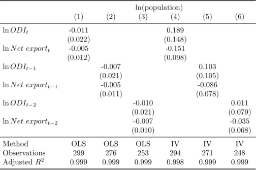
IV estimates could mitigate the first threat. Our strategy is to use foreign stock in China to be an instrument for Taiwan’s ODI in China and to use the trade between China and South Korea to be an instrument for trade between China and Taiwan. The instruments’

variables are

ODI_it^IV =X

j

Lijt−1

L_jt−1 S_jt^world

L_it−1 . (36)

N et export^IV_it =X

j

Lijt−1

L_jt−1 Ex^kr_jt L_it−1 −X

j

Lijt−1

L_jt−1 Im^kr_jt

L_it−1, (37) where S_jt^world represents the world’s ODI in China. Ex^kr_jt are exports from South Korea to China and Im^kr_jt are imports from China to

Korea. Different from OLS estimators, instrumental variables use em- ployment lagging behind one period to avoid the simultaneity bias (Autor et al., 2013).

We can avoid the second threat in a specific case of Taiwan and China. In this case, Taiwan experiences a positive demand shock from China. Firms could either increase exports or increase ODI to meet China’s demand. Either behavior would only be reflected in the observed changes of ODI or net exports.

4.2 Data

Taiwan’s approved yearly investment statistics in China were from the Taiwan Investment Commission. These are aggregate data at the 2-digit SIC industry level and include the agriculture, forestry, fish- ing, mining, manufacturing and service sectors. Investment amounts are deflated by the Personal Consumption Expenditures (PCE) index from the Bureau of Economic Analysis to the 2009 US dollar. Using the approved investment statistics, we measured ODI by the cumula- tive amount of investment. Assuming a 10% capital depreciation rate every year, we calculated ODI by the following equation,

ODIjt =

t

X

k=1991

(0.9)^t−kinvestment_jk. (38)

The data for the instruments of ODI were from the China Industry Economy Statistical Yearbook (CIESY), the AREMOS Cross-Strait Economic Statistics, the CEIC China Economic and Industry Data Database, as well as the China Trade and External Economic Statisti- cal Yearbook. CIESY contains the statistics of stocks at the firm-level, written as Actual Receipt Capital by Foreign Investors.⁷ Because it only recorded data from the manufacturing sector, the data of service sector were from the other three datasets. The complete data of all the industries were only available in the period from 1998 to 2010.

All RMB values were converted to US dollars by the yearly average exchange rate and were deflated by the PCE index.

The trade data were from the UN Comtrade database. In this database, Taiwan is labeled as ‘Other Asia, nes.’ Taiwan itself could not be identified. We compared the total trade value flow between China and Taiwan with those in the CEIC database, thereby confirm- ing that no other countries were included in the category ‘Other Asia,

7Only state-owned firms and private companies with annual revenues greater than 5 million RMB are recorded.

nes.’⁸ We used the raw data classified under the HS1992 commodity code at the 6-digit level, which we could map to the 2-digit SIC code to merge the data with individual-level data. Eventually we arrived at 20 industries, including the agriculture, forestry, fishing, mining, and manufacturing sectors. The conversion table comes from the UN Comtrade database. Values of imports and exports were deflated by the PCE index.

Our individual-level data were from the Manpower Utilization Sur- vey (MUS), which is a monthly national survey active since 1978. It investigates people ages 15 and above and includes both the labor force and the non-labor force. In this research, we restricted our sample to workers above 16 and below 64.

Our dependent variables were individual worker’s employment sta- tus and monthly wage. We constructed the dummy variable of unem- ployment by the definition of ‘narrow unemployment,’ which catego- rizes workers who are willing to work but not actively seeking employ- ment as part of the non-labor force instead of unemployed. Workers’

monthly wages were deflated by the Consumer Price Index from the Accounting and Statistics, R.O.C., and we used log of wage in all regressions.

We used demographic information as controls. Such controls in- cluded worker’s skill level, education level, marital status, age, job type, and working experience. Worker’s skill level was a dummy vari- able, defined as occupation. In MUS, occupation is classified into nine categories, which are ‘officials and managers,’ ‘professionals,’ ‘techni- cians,’ ‘sales,’ ‘office and clerical,’ ‘craft workers,’ ‘operatives,’ ‘labor- ers,’ and ‘service workers.’ We equated skilled labor with the first three categories, while equating unskilled labor with the others. Ed- ucation level was represented by dummies, which were categorized as under 6 years, 6 years, 9 years, 12 years, and above 12 years of school- ing. Marital status was constructed as a dummy variable, which was equal to 1 if one was married and living with a spouse and equal to 0 if one is single, divorced, or living separately from a spouse. Age and the square of age were both used as controls. A worker’s job type was defined as a full-time job or not, dependent on the weekly working hours (our cutoff point was 35). Experience was defined as the num-

8In fact, the statistics on trade values from Taiwan and those from China show differ- ences in the trade values. Chinas’ recorded values of Chinese exports are always higher than that those recorded by Taiwan. Likewise, China’s recorded values of Chinese im- ports are always lower than those recorded by Taiwan. According to Taiwan’s statistics, the trade surpluses only started appearing after 2001. Considering that statistics recorded by Taiwan were not classified at the industry level until 2004, we have no choice but to use the statistics from China.

ber of working years in the current job. Following Han et al. (2012), we used both experience and its square as controls.

To map the regional shocks to individual’s labor-market outcomes, we identified workers’ residential areas at the county level. We had 23 counties in total. A worker’s industry was classified under the 2-digit SIC code, which has three versions between 1998 and 2010. To make it consistent and so as to merge it with the ODI and trade data, we combined similar industries into one industry. We had 36 industries after combining.

We removed outliers with extreme wages. Following Autor et al.

(2008), we dropped observations with monthly wages lower than half the statutory minimum wage to ensure that the empirical results would be free from outlier effects. We deflated the wages to the price level in 2011, at which time half the minimum wage a month was NT$8940. Observations with monthly wages higher than one mil- lion were also dropped because they are all inaccurately recorded as 999,999 in MUS. These observations accounted for less than 0.05%

of the total sample in each year. Furthermore, we use the samples of manufacturing and service sectors because earnings in agriculture, forestry, fishing sectors are more likely to suffer measurement errors.

After pruning our dataset, we had 218,698 observations for males from 1998 to 2010.

In figure 1 and 2, we present the trends of ODI and net exports for high-exposure and low-exposure counties. As the figures show, the gap gradually widens, causing variations between counties. Three counties among the high-exposure counties are famous for their electronics and chemical manufacturing. Table 1 shows the summary statistics for individual-level data.

5 Empirical Results

5.1 Baseline Specification

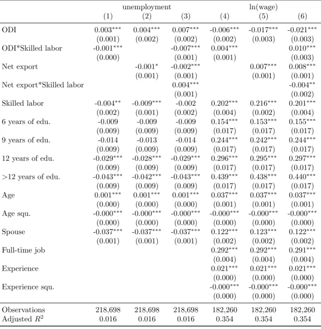
Table 2 reports the OLS results of the male labor market. The sam- ple period covers 1998 to 2010. The year fixed effects and the county fixed effects are included in all estimates. When interaction terms are excluded, ODI has a negative effect on both employment and wage level, while net exports have the opposite effect. Once we include the interaction terms for skilled labor, we find that skilled labor could be harmed from increased ODI and net exports in terms of both unem- ployment rate and wage level.

0 2 4 6 8 10 12 14

1998 2000 2002 2004 2006 2008 2010

Thousand dollars

Year

ODI of High- and Low-exposure Counties

high exposure low exposure

Figure 1: High-exposure (low-exposure) counties are the averages of ODI based on 6 counties, 25% of total 23 regions, with the highest (lowest) ODI exposure.

0 1 2 3 4 5 6 7 8 9

1998 2000 2002 2004 2006 2008 2010

Thousand dollars

Year

Net Exports of High- and Low-exposure Counties

high exposure low exposure

Figure 2: High-exposure (low-exposure) counties are the averages of net exports based on 6 counties, 25% of total 23 counties, with the highest (lowest) net export exposure.

Table 1: Summary Statistics

Variable Full sample

Observations 218,698

Percentage of unemployment (%) 4.11(19.85) Percentage of the skilled labor (%) 30.81(46.17) Percentage of under 6 years of schooling (%) 0.33(5.74) Percentage of 6 years of schooling (%) 10.98(31.27) Percentage of 9 years of schooling (%) 20.42(40.31) Percentage of 12 years of schooling (%) 36.76(48.21) Percentage of above 12 years of schooling (%) 31.51(46.45)

Age 39.06(10.64)

Percentage of having spouse (%) 65.49(47.54)

Wage sample

Observations 182,260

Wage (NT$) 44,597(27,061)

Percentage of the skilled labor (%) 32.39(46.79) Percentage of under 6 years of schooling (%) 0.33(5.74) Percentage of 6 years of schooling (%) 11.40(31.78) Percentage of 9 years of schooling (%) 20.23(40.17) Percentage of 12 years of schooling (%) 36.14(48.04 Percentage of above 12 years of schooling (%) 31.90(46.61)

Age 40.07(10.21)

Percentage of having spouse (%) 70.06(45.80) Percentage of having a full-time job (%) 95.18(21.42)

Experience (year) 9.12(7.96)

Standard errors in parentheses.

Table 2: The Impact of ODI and Trade on Male Labor Market

unemployment ln(wage)

(1) (2) (3) (4) (5) (6)

ODI 0.003^∗∗∗ 0.004^∗∗∗ 0.007^∗∗∗ -0.006^∗∗∗ -0.017^∗∗∗ -0.021^∗∗∗

(0.001) (0.002) (0.002) (0.002) (0.003) (0.003)

ODI*Skilled labor -0.001^∗∗∗ -0.007^∗∗∗ 0.004^∗∗∗ 0.010^∗∗∗

(0.000) (0.001) (0.001) (0.003)

Net export -0.001^∗ -0.002^∗∗∗ 0.007^∗∗∗ 0.008^∗∗∗

(0.001) (0.001) (0.001) (0.001)

Net export*Skilled labor 0.004^∗∗∗ -0.004^∗∗

(0.001) (0.002)

Skilled labor -0.004^∗∗ -0.009^∗∗∗ -0.002 0.202^∗∗∗ 0.216^∗∗∗ 0.201^∗∗∗

(0.002) (0.001) (0.002) (0.004) (0.002) (0.004) 6 years of edu. -0.009 -0.009 -0.009 0.154^∗∗∗ 0.153^∗∗∗ 0.155^∗∗∗

(0.009) (0.009) (0.009) (0.017) (0.017) (0.017) 9 years of edu. -0.014 -0.013 -0.014 0.244^∗∗∗ 0.242^∗∗∗ 0.244^∗∗∗

(0.009) (0.009) (0.009) (0.017) (0.017) (0.017) 12 years of edu. -0.029^∗∗∗ -0.028^∗∗∗ -0.029^∗∗∗ 0.296^∗∗∗ 0.295^∗∗∗ 0.297^∗∗∗

(0.009) (0.009) (0.009) (0.017) (0.017) (0.017)

>12 years of edu. -0.043^∗∗∗ -0.042^∗∗∗ -0.043^∗∗∗ 0.439^∗∗∗ 0.438^∗∗∗ 0.440^∗∗∗

(0.009) (0.009) (0.009) (0.017) (0.017) (0.017) Age 0.001^∗∗∗ 0.001^∗∗∗ 0.001^∗∗∗ 0.037^∗∗∗ 0.037^∗∗∗ 0.037^∗∗∗

(0.000) (0.000) (0.000) (0.001) (0.001) (0.001) Age squ. -0.000^∗∗∗ -0.000^∗∗∗ -0.000^∗∗∗ -0.000^∗∗∗ -0.000^∗∗∗ -0.000^∗∗∗

(0.000) (0.000) (0.000) (0.000) (0.000) (0.000) Spouse -0.037^∗∗∗ -0.037^∗∗∗ -0.037^∗∗∗ 0.122^∗∗∗ 0.123^∗∗∗ 0.122^∗∗∗

(0.001) (0.001) (0.001) (0.002) (0.002) (0.002)

Full-time job 0.292^∗∗∗ 0.292^∗∗∗ 0.291^∗∗∗

(0.004) (0.004) (0.004)

Experience 0.021^∗∗∗ 0.021^∗∗∗ 0.021^∗∗∗

(0.000) (0.000) (0.000)

Experience squ. -0.000^∗∗∗ -0.000^∗∗∗ -0.000^∗∗∗

(0.000) (0.000) (0.000) Observations 218,698 218,698 218,698 182,260 182,260 182,260

Adjusted R² 0.016 0.016 0.016 0.354 0.354 0.354

Standard errors adjusted for 299 clusters in year and county are in parentheses. ^∗ p < 0.1,

∗∗ p < 0.05, ^∗∗∗ p < 0.01. Year effects and county effects are included in all estimations.

The dummy of under 6 years of schooling is used as the control group.

5.2 IV estimates

We need instrumental variables due to the possibility of realized ODI, imports and exports being correlated with unobserved demand or sup- ply shocks from the home market. We use trade between South Korea and China as an instrument for that between Taiwan and China. We use the world’s stock in China as an IV for Taiwan’s ODI in China.

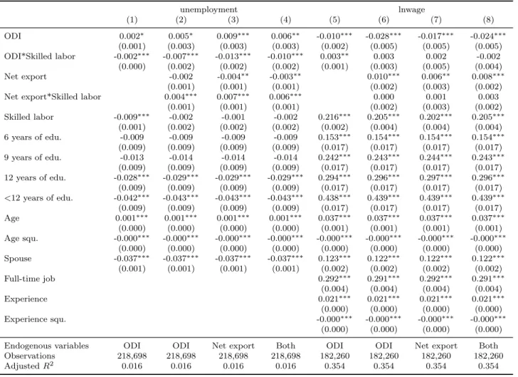
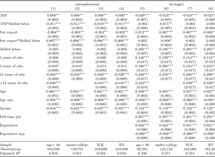
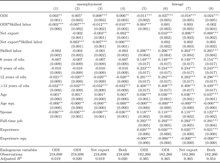
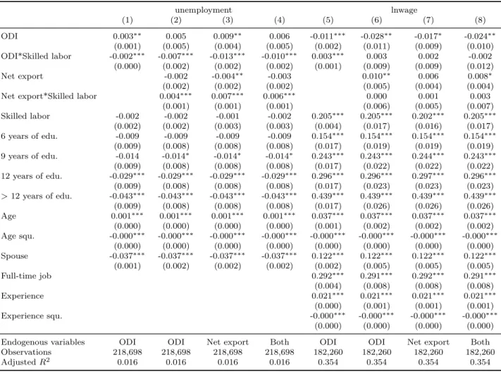
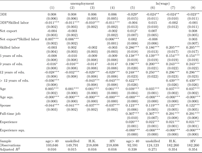
Table 3 presents the results of 2SLS estimates. For each depen- dent variable, we present four kinds of specifications. The coefficients are consistent within each specification. In the regression of unem- ployment, the coefficients show that increased ODI and net exports have opposite effects on unskilled and skilled labor. Unskilled workers benefit from increased net exports, while skilled ones benefit from in- creased ODI. As a brief conclusion to wage effects, ODI has negative effects on all of the labor force. The positive coefficients show that the skilled labor force suffers less, yet the effects are insignificant. Net exports have positive effects on all of the labor force. Similarly, the effects on skilled laborers are insignificant.

Most of the coefficients for the controls are statistically significant.

Other controls show that a man who with the college education and spouse is less likely to be unemployed and tends to have higher wage.

One who is older is more likely to be unemployed but has a higher wage. Men who have full-time jobs and more experience earn more.

And we see an inverted U-shape relationship between wage and age as well as between wage and experience.

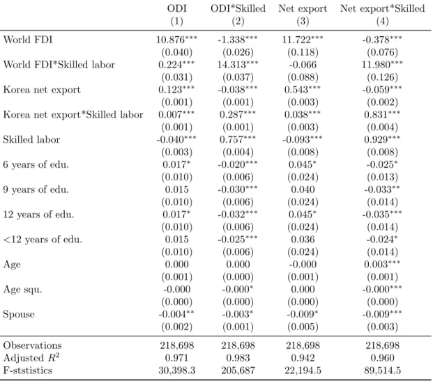
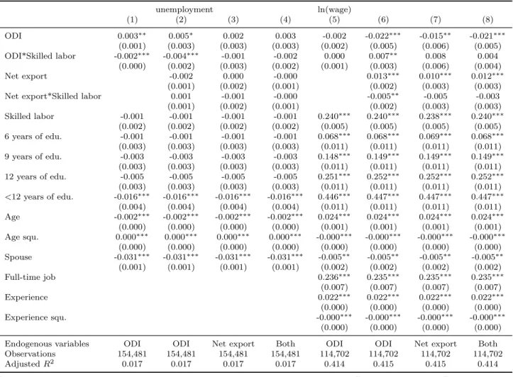
Table 4 reports the first-stage results. Here, both ODI and trade are treated as endogenous for the regression of unemployment. F- statistics are large, showing a strong relation between the instruments and endogenous variables.

To benchmark the impact, we applied the real values of ODI and net exports. Our preferred specification was the one that treated both ODI and net exports as endogenous. The unit of ODI is 1,000 dollars.

In other words, a 1,000 dollar increase in ODI led to a 0.6% increase in the unemployment rate by and a 2.4% decrease in the wage level for unskilled labor. For a skilled worker, the unemployment rate fell by 0.3%, and wage fell by 2.6%. The unit of net exports was also 1,000 dollars. For a 1,000 dollar increase in net exports, the probability of unemployment decreased by 0.3% for unskilled labor and increased by 0.3% for skilled labor. An unskilled laborer’s wage increased by 0.8%, and a skilled laborer’s wage rose by 1.1%. The average ODI rose from 1.42 in1998 to 5.97 in 2010, and the net export rose from 1.54 to 7.78.

As Table 5 shows, we applied the real changes in the values to the estimated coefficients. We also show, for comparison, the real changes in the unemployment rate and wage level between 1998 and 2010.