所得稅不確定性認列對公司決策的影響─以美國公司風險偏好及投資效率為例

國立臺灣大學管理學院會計學研究所 碩士論文

Graduate Institute of Accounting College of Management National Taiwan University

Master Thesis

所得稅不確定性認列對公司決策的影響─

以美國公司風險偏好及投資效率為例

The Impact of FIN 48 on Corporate Decision-Making─

Evidence from Risk-taking and Investment Efficiency of Firms in United States

黃中誠

Chung-Cheng Huang

指導教授：高偉娟 博士 林世銘 博士 Advisor: Wei-Chuan Kao, Ph.D.

Su-Ming Lin, Ph.D.

中華民國 106 年 6 月

June, 2017

致謝

在研究所的兩年學習過程裡，我要感謝家人作為我最大的支柱，讓我能夠在 臺大心無旁鶩的學習，另外也很慶幸自己能遇到許多熱心且有能力的同學們，一 起在報告跟撰寫論文的過程中相互鼓勵跟學習。

而碩士論文的完成，我更要非常感謝高偉娟老師的指導，無論任何問題都是 盡快回應學生，而且細心的說明，我才能一步步地完成這個論文。另外也要感謝 林世銘老師點出許多需要注意的細節，以及口試委員黃美祝老師和張祐慈老師寶 貴的意見，讓我的論文更臻完善。

最後，本研究亦感謝科技部「一般型研究計畫」(MOST 104-2410-H-002-050) 的支持。

摘要

本研究旨在瞭解美國第四十八號解釋公報對美國公司決策的影響。第四十八 號解釋公報從 2007 始適用，要求公司評估其稅務申報事項之不確定性，並以「未 認列租稅利益」之名詞進行揭露。既有文獻指出稅務風險會降低公司的風險偏好 程度。另外，較高的財務報表品質可以增加公司投資效率。本研究假設在第四十 八號解釋公報實施後，公司將會降低其風險承受的程度，同時投資效率將有所提 升。

實證結果顯示，從多個風險評估的變數觀察，公司確實在四十八號解釋公報 實施後降低了風險承擔的程度。足以證實四十八號解釋公報是公司無法迴避的稅 務風險。

再者，在第四十八號解釋公報實施後，趨向投資不足(過度)的公司增加(降低) 了投資的程度。而在較高資訊不對稱的環境下，投資效率增加的假設也獲得某些 面向的證據。

關鍵字: 四十八號解釋公報、未認列租稅利益、稅務風險、投資效率

ABSTRACT

This study is designed to test whether FIN 48 affects U.S. firms’ decision making.

FIN 48 effectively in 2007 requires companies to evaluate their uncertain tax positions and disclose the tax reserves as unrecognized tax benefits (UTBs). Then investors or stakeholders would know such tax risks. Additionally, prior literature indicates that tax risks make firms to reduce their risk-taking and that better financial reporting quality improves investment efficiency. If FIN 48, a required disclosure of tax risks, increase the exposure of tax risks and enhance financial reporting quality, firms would reduce their risk-taking and investment efficiency is improved in the FIN 48 regime. I examine such hypothesis by using a quasi-experiment method. The results show that firms reduces their operational risk-taking in the FIN 48 regime.

This suggests that FIN 48 expose firms with more tax risks and change firms’

decisions in risk-taking. Further results show that firms with propensity to

underinvestment (overinvestment) make more (less) investment in the FIN 48 regime, implying that FIN 48 reduces certain information asymmetry and thus improves firms’

investment efficiency.

Keywords: FIN 48; unrecognized tax benefits (UTBs); Tax risks; Investment efficiency

Contents

致謝... i

摘要... ii

ABSTRACT ... iii

Contents ... iv

List of Tables ... vi

1. Introduction ... 1

2.Relevant Literature and Hypothesis Development ... 4

2.1 Background ... 4

2.2 Tax Risks Affecting Corporate Decisions and Unrecognized Tax Benefit ... 5

2.3 Investment Efficiency and Unrecognized Tax Benefit ... 11

2.4 Research Hypothesis ... 14

3. Research Design ... 18

3.1 FIN 48 and Risk-taking ... 18

3.2 FIN 48 and Investment efficiency ... 22

3.3 Sample Selection ... 24

4. Empirical Results ... 25

4.1 Descriptive Statistics ... 25

4.2 Univariate Statistics... 29

4.2.1 T-test Between Treatment and Control groups ... 29

4.2.2 Pearson Correlation Coefficient ... 29

4.3 FIN 48 and Risk-taking ... 31

4.4 FIN 48 and Investment Efficiency ... 34

4.5.1 Effect of Information Asymmetry ... 37

4.5.2 Robustness Tests... 40

5. Conclusions, Constraints, and Recommendation ... 46

5.1 Conclusions ... 46

5.2 Constraints and Recommendation ... 46

APPENDIX A ... 48

References ... 52

List of Tables

Table 1 Descriptive Statistics...27

Table 2 Descriptive Statistics by Groups and T-test between treatment and control groups...28

Table 3 Pearson Correlation Coefficients...30

Table 4 FIN48 and Risk-taking ...33

Table 5 FIN 48 and Investment efficiency...36

Table 6 Additional Tests...39

Table 7 Robustness Tests 1...42

Table 8 Robustness Tests 2 ...44

1. Introduction

An interpretation of Financial Accounting Standards 109- Accounting for Income Taxes, FIN 48, is validated in 2007 demanding firms to provide information about uncertain tax positions in their financial reporting. It is natural that firms use tax strategies such as research tax credits and transfer pricing to decrease their income tax liabilities. However, those tax positions filed in tax returns will be audited and

challenged by tax authorities, some of which may not be sustained eventually. Before FIN 48 was adopted, tax uncertainty position is recorded in numerous ways. Financial Accounting Standards Board (FASB) considers it necessary to build a consistent guidance of income tax accounting, and thus introduce FIN 48. FASB believes that FIN 48 implementation improve financial reporting quality of income tax accounting.

Prior literature finds that FIN 48 affects firms’ financial reporting of tax reserves and income tax benefits since 2007. Researchers discuss FIN 48 from the perspective of relevance, management discretion, and market reactions (e.g., Ciconte et al. 2016;

Hanlon et al. 2017; Robinson et al. 2016; Gupta et al. 2016; Koester et al. 2015).

From a broader point of view, I would like to investigate how FIN 48 can affect firms’

decision making. Inspired by prior literature, I observe the impact of FIN 48 in terms of corporate risk-taking and investment efficiency.

First, previous literature suggests that tax risks have significant negative effects

on corporate risk-taking (e.g., Ljungqvist et al. 2016; Langenmayr and Lester 2015;

Guenther et al. 2017). Specifically, tax risks are widely documented as negative effects on reducing firms’ risk-taking in operations. The adjustments of risk-aversion toward tax risks for companies are expectable and reasonable. Considering FIN 48 as a stricter guidance for income tax accounting, I posit that FIN 48 exposes firms’ tax risk to their stakeholders, so firms will reduce their risk-taking in the FIN 48 regime.

On the other hand, some literature provides evidence that better financial reporting quality leads to investment efficiency (e.g., Biddle et al. 2009; Lara et al. 2015). In

spite of the mixed findings for whether FIN 48 can improve financial reporting quality, I am supportive of FASB’s positive opinion on FIN 48. Therefore, I hypothesize that

investment efficiency is enhanced in the FIN 48 regime.

To test the corporate risk-taking, I mainly follow the work of Ljungqvist et al.

(2016) and then use four different proxies to understand how the implementation of FIN48 affects firms’ risk-taking. As for the method of analyzing investment efficiency,

I refer to Lara et al. (2015). The measure for underinvestment (overinvestment) is generated from deciled industry-year residuals of the regression of aggregate investments on sales growth.

Using U.S. firms from 1990 to 2015, the empirical results mainly support my hypotheses. To begin with, all four proxies for the risk-taking of firms with UTB

inherent decrease in the FIN 48 regime. The evidence is consistent and strong so that the inference of FIN 48 representing a tax risk for companies is corroborated. Next, I observe higher (lower) level of investment for firms with UTB inherent and higher propensity toward underinvestment (overinvestment). The outcome is mostly

consistent in that three out of four (all four) measures of investment are significantly increased (decreased). Additionally, the setting of information asymmetry contributes some evidence. With higher information asymmetry, the level of investment for companies with UTB and tendency towards underinvestment (overinvestment) has risen (dropped). These findings confirm that FIN 48 is effective in improving financial reporting quality in the sense that investment efficiency becomes better.

This study is the first to integrate FIN 48 with tax risk and investment efficiency expanding the existing literature on FIN 48. Little literature of FIN 48 is focused on specific corporate decision-making. Finally, it is worth noticing for policy makers that FIN 48 has some economic consequences.

2.Relevant Literature and Hypothesis Development

2.1 Background

Prior to the enactment of FIN 48, firms report taxes in the financial statements following Financial Accounting Standard No.109 (SFAS 109), Accounting for Income Tax. However, SFAS 109 contains no specific guidance for tax uncertainty. Hence, firms usually address uncertain tax positions by using Financial Accounting Standard No.5 (SFAS 5), Accounting for Contingencies. No explicit instruction regarding accounting for tax uncertainty leads to diverse accounting practices. FASB therefore issues FIN48 to improve the relevance and comparability in financial reporting of income taxes hoping that the principles would provide consistent recognition and measurement.

FASB states that FIN 48 improves financial reporting for uncertain tax positions, namely tax reserves (FASB 2006). FIN 48 requires firms to report tax reserves

following two steps. First, FIN 48 asks companies to evaluate the position pursuant to the more-likely-than-not recognition threshold. Second, a tax position that meets the more-likely-than-not recognition threshold shall be measured as the largest amount of tax benefit that is greater than 50 percent likely of being realized upon settlement with a taxing authority that has full knowledge of all relevant information. At the same time, firms are required to disclose more information about firms’ tax uncertainty.

These two steps provide uniform guidance for firms to follow. Meanwhile, FIN 48 defines the difference between the recognized income tax benefit and the amount filed in the tax returns as unrecognized tax benefits (UTBs).

According to the exposure draft of FIN 48 (FASB 2005), there are two board members with an alternative view. They were concerned that FIN 48 would be needlessly complex and difficult to apply in practice. Specifically, companies might systematically overstate tax reserves at first and then reverse these recorded liabilities when the tax authority finishes auditing their tax position. This debate triggers more tension about whether FIN 48 reduces information asymmetry, improves financial reporting quality, and further improves investment efficiency. Additionally, how FIN 48 affect corporate risk-taking is unclear, and therefore how FIN48 affects investment efficiency is still an empirical question.

2.2 Tax Risks Affecting Corporate Decisions and Unrecognized Tax Benefit

Firms are faced with various risks such as operational risks, financial risks, et

cetera. Among these risks, tax is one of those that should be taken into consideration in the process of firms’ every critical decision making. The survey undertaken by Ernst &

Young (2014) points out four sources of tax risks that tax and financial executives are concerned about. They are reputation risk, the base erosion and profit shifting (BEPS)

risk, enforcement risk, and operational risk. Taking transfer pricing as an example, a multinational company takes advantage of its global supply chain and transaction arrangements to reduce its overall tax burden. However, since OECD proposed BEPS actions, aggressive tax avoidance has become an issue. Thus, multinational companies have been under the pressure from different jurisdictions. These companies would have more compliance costs when planning transfer pricing, and have higher possibilities of

double taxation that required their attention to adjust their operations. According to PwC’s global CEO survey (2015), over half of the CEOs say: “governments on a global

basis are increasingly implementing more competitive tax policies, which influence organizations’ decisions on where to operate.”

Prior literature echoes the practitioners’ findings and demonstrates how tax risk

affect overall firm risk (e.g. Ljungqvist et al. 2016; Langenmayr and Lester 2015;

Guenther et al. 2017; Hutchens and Rego 2015). First, Ljungqvist et al. (2016) find that firms respond to tax risks by reducing the risk-taking when their home state tax

increases. To be precise, the signal of risk reduction is the decrease in earnings volatility, and the change of operating cycle. Consistent with lower earnings volatility, the days of operating cycle are shorter. Besides, Langenmayr and Lester (2015) use both a

theoretical and an empirical model to ascertain the effect of tax rules on corporate risk-taking. The tax rules in this literature refer to tax loss offset and statutory tax rates.

The level of corporate risk-taking increases if the available loss offset period is longer.

The effects of tax rates on risk-taking are opposite for firms with high or limited possibilities of using their loss offset. Higher rates lead to greater risk-taking for firms expecting to use the loss offset, but the relation is negative for firms unlikely to the loss offset.

Moreover, Guenther et al. (2017) test whether corporate tax avoidance strategies are related to higher risks in the future and find mixed results. They do not find association between historical tax avoidance behaviors and future firm risks measured by cash tax rate volatility or stock return volatility. However, the results show a

significant relationship between tax rate volatility and stock return volatility, a measure of overall firm risk. A similar finding can be referred to in Hutchens and Rego (2015).

Hutchens and Rego (2015) use several proxies for tax risk and firm risk to test the relation between the two kinds of risk. The results suggest that discretionary book-tax differences and cash effective tax rate volatilities are positively associated with all of their proxies for firm risk. Last, just as Donohoe et al. (2014) describe, tax departments act as risk centers after the validation of FIN 48 and the use of schedule UTP.

The change in overall firm risk can stand for a signal of firms changing their operations or the process of decision-making. In order to further understand what tax risk can have any effect specifically, I explore the following literature (Chow et al.

2016; Alexander and Jacob 2016; Graham et al. 2016; Jacob et al. 2016)

Chow et al. (2016) examine the relation between the takeover premiums acquirer willing to pay and target companies’ tax sheltering behavior. On average, there are 4.6

percent higher premiums for target companies when they disclose they do not engage in tax sheltering. The result shows that acquirers prefer less tax risks when undergoing mergers and acquisitions. Alexander and Jacob (2016) interpret how tax risks interact with managers’ inside debt (i.e. pension plans and deferred compensation of high

executives). They find the high executives tend to be more risk-averse toward companies’ uncertain tax position if inside debt level is greater. Graham et al. (2016)

conduct a survey to ask tax executives which tax rate their companies use as an input when making corporate decisions. According to the corporate finance theory, marginal tax rate is preferable, which is defined as the present value of additional taxes paid on an additional dollar of income earned today (Scholes et al. 2014). The survey shows that fewer than 13% of their sample firms use the marginal tax rate in any

decision-making. Graham et al. (2016) then test whether the theoretically incorrect choice of tax rate leads to suboptimal decision-making. For capital structure, they find that firms with marginal tax rate (MTR) greater than GAAP effective tax rate (ETR) use more conservative debt policies. As for investments, firms with larger gap between MTR and GAAP ETR are less responsive or efficiency in investment

arrangements. Jacob et al. (2016) also document how tax uncertainty affects corporate investment decisions. Their measures for tax uncertainty contain GAAP ETR

volatility, ending balance of UTB scaled by total assets, and estimated cash buffer due to increases in ETR volatility. The results suggest that tax uncertainty leads to the delay of large investments and lower levels of investments.

As for the studies for unrecognized tax benefits, some literature discusses

whether FIN 48 change managements’ discretion over tax uncertainty (e.g. Gupta et al.

2016; Robinson et al. 2016). Prior to the adoption of FIN 48, there was great complexity inherent in tax expense itself, and managers had quite large discretion about reporting tax contingency. According to the anecdotal information provided in Blouin et al. (2010), KPMG’s policy was to require clients to record a contingency unless they had more than 70 percent chance surviving IRS’s challenges. Other

companies used an expected value approach to record tax contingency to minimize the average impact on earnings when they settled with tax authorities. To sum up, there is divergence in the practice prior to the enactment of FIN 48.

The factors mentioned above give opportunities for earnings management.

Dhaliwal et al. (2004) observe that firms tend to decrease their annual GAAP effective tax rate if they fall short of analysts’ forecasts. However, Gupta et al. (2016) find that,

compared to the period prior to FIN 48, firms reduce earnings management through

tax reserve in the period following the adoption of FIN 48. Moreover, Robinson et al.

(2016) interpret that the restrictions of FIN 48 prevent the management from bringing more private information.

Previously researchers observe the positive market reactions to the adoption of FIN 48 (e.g. Koester et al. 2015). Dyreng et al. (2016) further suggest tax avoidance increase UTBs. Meanwhile, the market affirmatively value tax avoidance because tax avoidance means that managers could pay less cash tax to the government. Nesbitt et al.

(2016) takes advantage of the Luxembourg tax leaks event and test the market reaction using three-day window abnormal return model. On average, the market reacted positively toward the Luxembourg tax leaks event, which released information of firms engaging in tax avoidance. Specifically, Koester et al. (2015) find a positive relation between stock price and the disclosure of UTB. Although the positive effect is attenuated if tax-related material weakness in internal controls is in presence. The rational possible interpretation for the positive market reaction is that the balance of

UTB serves as a signal of tax avoidance. On the other hand, FIN 48 has a large impact on firms’ behaviors of compliance (e.g. Gupta et al. 2014; Blouin et al. 2007). Gupta et

al. (2014) documents that both firm-level tax expense and state-level tax collections increase under the FIN 48 regime which shows the change of financial reporting standards can affect firms’ behaviors pertaining to tax. That is, tax avoidance is

attenuated to certain degree. Considering tax avoidance as the reason of UTB receiving positive market reaction, perhaps the findings of Koester et al. (2015) are short-term phenomena. As tax avoidance decreases in the FIN 48 regime, the positive market reactions may also decline. Last, Blouin et al. (2007) hand-collected 100 largest non–

financial and non–regulated firms’ disclosures of tax reserve. All of them report the

balance of UTB on January 1, 2007.

Overall, there still hasn’t any literature to argue whether FIN 48 represents a tax

risk for companies and will affect their risk-taking.

2.3 Investment Efficiency and Unrecognized Tax Benefit

Prior research finds that FIN 48 provides predictability of future cash flows for financial reporting users (e.g., Ciconte et al. 2016; Hanlon et al. 2017). Specifically, Ciconte et al. (2016) find a positive relation between UTB and future income tax cash outflows after the adoption of FIN 48, suggesting that the recognition improves the predictability of income tax cash flows. Hanlon et al. (2017) find that firms with higher tax uncertainty hold larger levels of cash using the balance of UTB scaled by total assets as the measure of tax uncertainty. This result suggests that UTB can be used to predict a companies’ future cash positions. Nevertheless, Robinson et al. (2016) argue that the fixed rules of FIN 48 fail to improve the relevance of income tax accounting.

They find no evidence that the predictive ability of tax expense for future tax outflows

improves. This result is clearly contradictory to that of Ciconte et al. (2016). This inconsistency could result from different proxies for predictability. Still, mixed evidence exists about whether FIN 48 improve the quality of accounting for income taxes. Hence, I would like to investigate the association between FIN 48 and financial reporting quality through investment efficiency.

Based on prior discussion, there is profound evidence supporting that financial reporting quality influences firms’ investment decisions. Furthermore, investment

efficiency improves by virtue of less information asymmetry (e.g. Biddle et al. 2009;

Lara et al. 2015). It means that the core concept linking financial reporting quality and investment efficiency is information asymmetry. First, the information asymmetry between firms and investors can be described as a source of adverse selection. The adverse selection problem may increase the cost of raising capital and hence lead to under-investments. For example, Myers and Majluf (1984) prove that there are some situations in which firms would probably forgo projects with positive NPV if the management acts in favor of existing shareholders. It means management giving up positive investments when the capital comes from issuing stock at a discounted price.

Secondly, the agency problem (Jensen and Meckling 1976) may cause greater cost of raising capital or poor project selection and therefore result in under- or over- investments. Companies’ managers sometimes do not make the most beneficial

decisions in those situations where they have opportunities of seeking personal interests. There are several likely scenarios. For instance, managers over-invest to meet certain benchmarks required in their contracts so that they can gain the compensation (Jensen 1986). On the other hand, Bertrand and Mullainathan (2003) using plant-level data find that average managers tend not to build new plants if their firms are protected from hostile takeovers by the law. Lambert et al. (2007) give us an

insight that better information reduces a firm's cost of capital which they define as the expected return on a firm’s stock. Putting it in another way, the information

asymmetry may leave shareholders cautious beforehand which gives rise to under-investment ex-post.

However, better financial reporting quality can alleviate information asymmetry and reduce the costs of adverse selection and agency problems. Leuz and Verrecchia (2000) study German firms which change their financial reporting from German to an international regime (i.e. IAS or U.S. GAAP). They document lower bid-ask spread and higher share turnover for firms adopting international IAS or U.S. GAAP.

Following the logic, accounting conservatism aids in mitigating agency costs. Early or timely loss recognition discipline managers to invest more prudently. If managers tend to over-invest beyond the optimal level, they are more likely to suffer from those inadequate investments due to the early loss recognition. Francis and Martin (2010)

discover that the positive relation between timely loss recognition and acquisition profitability is stronger for firms with larger ex-ante agency costs.

Providing more direct evidence about financial reporting quality and investment efficiency, Biddle et al. (2009) observe that, with higher financial reporting quality, investment efficiency improves. To be precise, the investment level of firms with better likelihood of over-investment (under-investment) decreases (increases) if financial reporting quality gets higher. Lara et al. (2015) further test investment efficiency by incorporating the effect of conservatism and settings of information asymmetry. Their findings are consistent with those of Biddle et al. (2009) and even more robust. More conservative firms invest more if inclined toward underinvestment.

The positive effect of conservatism remains in each scenario for which Lara et al.

(2015) use different proxies for information asymmetry. Also, Cheng et al. (2013) examines firms that have poor financial reporting quality prior to the first disclosure of an material internal control weakness (ICW). They find that ICW firms over-invest (under-invest), relative to non-ICW firms, if they are more prone to over-investment (under-investment).

2.4 Research Hypothesis

The primary objective of this study is to interpret how FIN 48 can affect firms’

processes of decision-making among which risk-taking and investment efficiency

draw my attention most.

To begin with, prior literature indicates positive or mixed evidence that tax risk influences corporate risk-taking. Ljungqvist et al. (2016) find negative association between state tax increases in the U.S. and firms’ risk-taking. Langenmayr and Lester (2015) indicate that more generous tax loss provision induces firms’ risk-taking, especially when the firms are in the country with higher statutory tax rates. Guenther et al. (2017) further observe a significant link between tax rate volatility and stock return volatility while they do not capture their expected positive relation between tax avoidance and future firm risk.

Although there is no precise definition for tax risk, I regard it as the uncertainty that will change firms’ operations. As regulations grow rapidly these days, it’s

inevitable that firms need to carefully manage their risks in taxation. It occurs to me that FIN 48 is the most significant financial reporting rule for tax accounting recently.

Not to mention the core concept of FIN 48 is disclosing uncertain tax positions, the update of this rule itself can be a risk. Hence, I anticipate FIN 48 to have a positive impact on corporate risk-taking. Gupta et al. (2014) already observes less tax avoidance in FIN 48 regime. Their finding is a sign of firms lowering their risks pertaining to tax. It’s reasonable to infer that other aspects of risk are reduced in the meantime. Hence, I state my first hypothesis in alternative form as follows:

H1: Firms reduce their risk-taking in the FIN 48 regime.

Biddle et al. (2009) and Lara et al. (2015) suggest that better financial reporting quality improves investment efficiency because of less information asymmetry.

Balakrishnan et al. (2012) explains that the complexity and uncertainty inherent in tax planning generate opacity between firms and their stakeholders, leading to information asymmetry problems. Then, the question of interest is whether FIN 48 can enhance financial reporting quality, lessen information asymmetry, and therefore improve investment efficiency. Ciconte et al. (2016) and Hanlon et al (2017) indicate that FIN 48 provides financial reporting users with predictability of tax cash flows. On the other hand, Robinson et al. (2016) argue that FIN 48 is not able to improve the relevance of income tax expense.

Despite the fact that conflicting opinions exist for whether FIN 48 enhance financial reporting quality, I posit that more information regarding tax reserve is provided. Especially, IRS statistics from 2010 to 2014 show that the top two uncertain tax positions reported by filers are R&D tax credit, and transfer pricing. Capitalization ranks as either the third or the fourth¹. In this sense, the disclosure of UTBs can reflect the eventual tax effects on corporate investment decisions to a certain degree since R&D and capitalization are regarded as sources of investments. With the incremental

1 Statistics for uncertain tax positions are available on the IRS website:

information provided by the disclosure of UTB and lower level of tax avoidance in the FIN 48 regime, I expect the information asymmetry problems to be alleviated. The cost of a tradeoff between the financial reporting quality and corporate investment decisions becomes smaller. Hence, I expect FIN 48 to enhance firms’ financial reporting quality and improve their investment efficiency. The above discussion leads to my second hypothesis in alternative form:

H2: Among firms prone to underinvestment (overinvestment), the firms with UTB

inherent invest more(less) in the FIN 48 regime.

3. Research Design

3.1 FIN 48 and Risk-taking

To test the first hypothesis, I set up the following regression model (time and firm subscripts suppressed for brevity):

𝑅𝑖𝑠𝑘𝑠 = 𝛽₀+ 𝛽₁𝑈𝑇𝐵 + 𝛽₂𝑃𝑂𝑆𝑇07 + 𝛽₃ 𝑈𝑇𝐵 ∗ 𝑃𝑂𝑆𝑇07 + 𝑿’𝜁 + 𝑖 + 𝑡 + 𝜀 (1) 𝑿 stands for control variables. I also control for industry (i) and year (t) fixed effects.

I use the 48 industry classifications in Fama and French (1997) for the industry fixed effect. To evaluate the risk-taking of firms, I follow the work of Ljungqvist et al. (2016).

They offer several measures to proxy for the dependent variable Risks. Those measures include ROA volatility, ROIC volatility, Operating Cycle Change Ratio, and Capex. ROA

volatility is the standard deviation of quarterly pretax returns on assets and ROIC

volatility is the standard deviation of quarterly pretax returns on invested capital. Both are

calculated over the period from t to t+2. They both are suitable proxies to reflect firms’

aggregate risk taking. Operating Cycle Change Ratio is the ratio of the difference

between current and one-year ahead operating cycle to current operating cycle. This ratio is expected to detect whether firms reduce their risk-taking by shortening their operations.

If operating cycles are shorten, the operating capital put in risk becomes less. Capex in my definition is one-year ahead net capital expenditure (capital expenditure less sale of property) over the book value of lagged total assets.

UTB is an indicator variable equal to one if an observation has any data in the

following items that are provided in Compustat: beginning balance of unrecognized tax benefits, ending balance of unrecognized tax benefits, decreases to unrecognized tax benefits relating to settlements with taxing authorities, interest and penalties related to uncertain tax positions, and increases to unrecognized tax benefits arising from uncertain tax positions taken in a prior year. POST07 is equal to one if an observation is in 2007 or afterwards, and zero otherwise. 2007 is the year when FIN 48 is validated. My main independent variable is UTB*POST07, the interaction effect of UTB and POST07. As my first hypothesis states, I expect β3 to be negative because I argue that firms reduce their risk-taking in the FIN 48 regime.

Following prior literature, I include the firm characteristics that may affect firms’

investment and financing activities as control variables (e.g. Fama and French 1993 1995 2002; Harris and Raviv 1991; Coles et al. 2006; Jackson et al. 2009; Dechow and Dichev 2002; Liu and Wysocki 2016; Kothari et al. 2005). Specifically, I control for leverage (LEV), the accounting method choice of depreciation (DEP_PUREAC), the log of firm age (LOGAGE), market-to-book value (MTB), the log of market value of equity (LOGMVE), the volatility of sales (STDSALES), the volatility of investments

(STDINVEST), the log of operating cycle (LOGOPCYCLE), and

performance-matched modified-Jones model discretionary accrual (PERFDAROA).

(1) LEV stands for leverage, equal to long-term debt divided by common equity. A large stream of finance literature illustrates the corporate capital structure decisions (e.g. Fama and French 2002; Harris and Raviv 1991). Meanwhile, Coles et al. (2006) find positive relation between leverage and CEO

compensation schemes with higher sensitivity to stock volatility. In light of the literature, I believe the choices of capital structure are made to optimize the firm value. Hence, leverage is a cumulative outcome of corporate decisions and will positively affect firms’ risk-taking.

(2) DEP_PUREAC is an indicator showing whether the firm adopts the accounting method choice of accelerated depreciation or the units of production method.

Jackson et al. (2009) find that the external financial reporting choice of

depreciation method affects managerial decisions on capital investments. Firms using accelerated depreciation make larger investments than firms that use straight-line depreciation. Thus, I argue that the aggressive choice of depreciation method has an positive impact on firms’ risks ex ante.

(3) LOGAGE is the log of firm age. MTB is market-to-book value. LOGMVE is log of market value of equity which proxies for firm size. These variables are common variables to control for firm-level characteristics. First, the nature of firms’ operations changes as they grow so firms’ age can capture their

developments over time. I expect LOGAGE to have negative effects on

risk-taking for firms’ development may become stable as they grow. Secondly, Fama and French (1993) find evidence that size and market-to-book equity proxy for sensitivity to risk factors in stock returns. Furthermore, market-to-book value can be an indicator of the growth opportunities since firms with higher

market-to-book value are typical of higher average returns (growth stocks) and strong earnings ( Fama and French 1995). Therefore, I suppose that MTB and

LOGMVE are positively associated with my proxies for corporate risks.

(4) STDSALES and STDINVEST represent the volatility of sales and investments.

These two variables proxy for firms’ historic operating volatilities.

LOGOPCYCLE is the log of operating cycle. Prior literature (e.g. Dechow and

Dichev 2002; Liu and Wysocki 2016) provides evidence that these operating features affect accruals quality. In light of their work, a portion of operating decisions come along spontaneously and are without managerial discretions such

as accounting principle choices. Hence, I expect these variables to capture some variation of firms’ risk-taking and the effects are positive. Higher operating

volatilities and longer operating cycles are indicators of higher risk-taking.

(5) PERFDAROA is the performance-matched modified-Jones model discretionary

accrual developed by Kothari et al. (2005)². It’s a proxy for financial reporting quality in the sense that larger value of PERFDAROA refers to poorer quality of

financial reporting. Francis et al. (2005) conclude that accruals quality is a risk factor priced by investors. Given this idea, I suppose it’s necessary to control for

the reporting quality. The relation may be positive because firms need to react to capital providers’ higher required rate of return for higher information risk

brought out by poor accrual quality.

The detailed definitions of variables can be referred to in appendix A.

3.2 FIN 48 and Investment efficiency

To test my second hypothesis, I extend equation (1) to the following equation:

𝐼𝑁𝑉𝐸𝑆𝑇𝑀𝐸𝑁𝑇 = 𝛽₀+ 𝛽₁𝑈𝑇𝐵 + 𝛽₂𝑃𝑂𝑆𝑇07 + 𝛽₃𝑈𝑁𝐷𝐸𝑅𝐼𝑁𝑉𝐸𝑆𝑇

+𝛽₄𝑂𝑉𝐸𝑅𝐼𝑁𝑉𝐸𝑆𝑇 + 𝛽₅𝑈𝑇𝐵 ∗ 𝑃𝑂𝑆𝑇07 + 𝛽₆𝑈𝑇𝐵 ∗ 𝑃𝑂𝑆𝑇07

∗ 𝑈𝑁𝐷𝐸𝑅𝐼𝑁𝑉𝐸𝑆𝑇 + 𝛽₇𝑈𝑇𝐵 ∗ 𝑃𝑂𝑆𝑇07 ∗ 𝑂𝑉𝐸𝑅𝐼𝑁𝑉𝐸𝑆𝑇

+𝑿’𝜁 + 𝑖 + 𝑡 + 𝜀, (2) where 𝑿 stands for the same control variables as equation (1) plus OVERINVEST*

PERFDAROA and UNDERINVEST* PERFDAROA. The expected effects of the

2 First, discretionary accruals are generated from estimating modified-Jones model as follows:

Acct=α + β1 (△Revt -△Rect)+β2 PPEt + εt

Then, the performance-matched discretionary accrual is calculated as the difference between the discretionary accruals of matched firms. That is:

control variables are also the same except LOGMVE. I think its coefficient would be negative since the proportion of investment is unlikely to stay as high after companies grow larger. Industry and year fixed effects are controlled. I use four different

measures to evaluate firms’ investment as the dependent variable. The first kind is the one used in Biddle et al. (2009) which is the one-year ahead sum of research and development expenditure, capital expenditure, and acquisition expenditure, less cash receipts from the sale of property, plant, and equipment and scaled by lagged total assets (Investment_latf1). Secondly, I modify the first measure to a simpler one which is the one-year ahead sum of research and development expenditure and capital expenditure and then scaled by lagged total assets. (Investment2_f1). Last, I also test the ratio of one-year ahead capital expenditure to lagged total assets (Capex) and the ratio of one-year ahead research and development expenditure to lagged total assets (R&D spending). The development of UNDERINVEST and OVERERINVEST is based on the work of Lara et al. (2015). The first step is to estimate the regression model of aggregate investments on sales growth on industry-year levels. The second step is to rank the residuals of the equation into deciles and multiply them by -1. Then, I rescale them to range from 0.1 to 1. The larger value in this range, the more likely a firm is to underinvest. Finally, I define the group with the value of 1 as UNDERINVEST and the group with the value of 0.1 as OVERINVEST. In this test, the main independent

variable of interest is UTB*POST07*UNDERINVEST and

UTB*POST07*OVERINVEST. Anticipating firms prone to underinvestment

(overinvestment) and with UTB inherent invest more (less) in the FIN 48 regime, I posit that β6 (β7) is to be positive (negative).

3.3 Sample Selection

The sample is the publicly-traded U.S. firms from Compustat database. My sample includes firms between fiscal year 1990 and 2015. I drop firms in the electric, gas and sanitary services sector (SIC 4900 to 4999) and finance, insurance and real estate (SIC 6000 to 6799), because these firm have different firm characteristics. I also delete the observations with missing data. Last, I winsorized the variables in my tests lying beyond the 1% or 99% range of the sample distribution.

4. Empirical Results

4.1 Descriptive Statistics

Table 1 provides descriptive statistics for my main and control variables. To start with the main variables, the average (median) ROA volatility is 7.1% (1.5%), and the average (median) ROIC volatility is 16.1% (2.2%). The average (median) Operating

Cycle Change Ratio is 1.9% (-2.1%). The absolute difference between the average

and absolute value isn’t huge but the direction is opposite. Besides, the standard deviation is enormous. Operating Cycle Change Ratio reflects volatile and random business environments. The average (median) Investment_latf1 is 16.1% (8.9%) and

the average (median) Investment2_f1 is 12.9% (7.1%). They both seem able to capture firms’ relative investment levels to the total assets. The mean UTB is 11.8% which

stands for the portion of the treatment group. Table 2 provides descriptive statistics for firms with UTB as the treatment group and firms without UTB as the control group.

First, firms in the treatment group are more risk-averse than those in the control group.

This observation can be made by comparing the treatment and control groups in the same period. To be precise, the comparison is between firms with and without UTB before (after) 2007.The mean value and the standard deviation of ROA volatility,

ROIC volatility, Operating Cycle Change Ratio, Capex, STDSALES, STDINVEST,

and LOGOPCYCLE are mostly smaller in the treatment group no matter they are

before or after 2007. Secondly, the mean value of Operating Cycle Change Ratio and

Capex become less after 2007 for firms with UTB. These results represent primitive

evidence on firms reducing their risks and make changes to simplify their operations.

However, some variables do not bring about the same outcome (e.g. ROA volatility, and ROIC volatility). Therefore, more evidence is needed to support my expectations.

Table 1 Descriptive Statistics

N Mean Std Dev Min P25 P50 P75 Max

ROA volatility

122988 0.071 0.268 0.001 0.007 0.015 0.036 2.296

ROIC volatility

123059 0.161 0.597 0.002 0.010 0.022 0.055 4.634

Operating Cycle

Change Ratio

107774 0.019 1.908 -9.293 -0.206 -0.021 0.140 11.884

Capex

108546 0.058 0.082 -0.041 0.013 0.033 0.071 0.530

Investment_latf1

110490 0.161 0.233 -0.037 0.035 0.089 0.189 1.543

Investment2_f1

110215 0.129 0.187 -0.029 0.028 0.071 0.151 1.230

R&D spending

109187 0.068 0.156 0.000 0.000 0.000 0.068 1.034

UTB

123263 0.118 0.323 0.000 0.000 0.000 0.000 1.000

POST07

123263 0.308 0.462 0.000 0.000 0.000 1.000 1.000

OVERINVEST

108895 0.100 0.300 0.000 0.000 0.000 0.000 1.000

UNDERINVEST

108895 0.084 0.278 0.000 0.000 0.000 0.000 1.000

LEV

123263 0.206 0.292 0.000 0.000 0.105 0.298 1.738

DEP_PUREAC

123263 0.019 0.137 0.000 0.000 0.000 0.000 1.000

LOGAGE

123263 2.607 0.706 1.386 2.079 2.565 3.135 4.190

MTB

123263 2.575 6.666 -27.826 0.884 1.758 3.327 39.443

LOGMVE

123263 4.945 2.621 -1.143 3.071 4.912 6.783 11.043

STDSALES

123263 0.462 0.876 0.000 0.102 0.213 0.449 6.807

STDINVEST

123263 0.219 0.568 0.000 0.028 0.067 0.166 4.524

LOGOPCYCLE

102463 4.127 1.330 -6.798 3.677 4.350 4.891 7.196

PERFDAROA

114194 0.043 2.204 -10.963 -0.132 -0.001 0.134 12.663

IA_Spread

103392 0.409 0.215 0.100 0.200 0.400 0.600 1.000

Table 2 Descriptive Statistics by Groups and T-test between treatment and control groups

UTB=1 n

1

=10,688 UTB=0 n

2

=61,689

T-test between treatment and control groups n=72,377 Before 2007

n

1b

=5,368

Post 2007 n

1p

=5,320

Before 2007 n

2b

=47,233

Post 2007 n

2p

=14,456

Mean Std Dev Mean Std Dev Mean Std Dev Mean Std Dev Difference t-statistic

ROA volatility

0.019 0.030 0.020 0.069 0.026 0.064 0.022 0.066 -0.00578*** (-8.78)

ROIC volatility

0.039 0.169 0.056 0.283 0.058 0.264 0.057 0.278 -0.0107*** (-3.88)

Operating Cycle

Change Ratio

0.037 1.143 0.029 1.163 0.032 1.532 0.078 1.570 -0.00976 (-0.63)

Capex

0.058 0.065 0.039 0.044 0.057 0.069 0.047 0.059 -0.00618*** (-9.01)

Investment_latf1

0.162 0.190 0.147 0.179 0.147 0.187 0.132 0.170 0.0115*** (5.98)

Investment2_f1

0.117 0.129 0.106 0.125 0.114 0.138 0.101 0.127 0.000451 (0.32)

R&D spending

0.058 0.107 0.067 0.120 0.056 0.114 0.054 0.116 0.00713*** (5.95)

OVERINVEST

0.078 0.269 0.073 0.261 0.068 0.252 0.065 0.247 0.00835** (3.15)

UNDERINVEST

0.041 0.199 0.053 0.224 0.079 0.270 0.080 0.271 -0.0325*** (-11.81)

LEV

0.192 0.245 0.195 0.260 0.192 0.246 0.181 0.234 0.00392 (1.53)

DEP_PUREAC

0.013 0.112 0.002 0.041 0.017 0.129 0.007 0.082 -0.00727*** (-6.04)

LOGAGE

2.476 0.713 2.643 0.636 2.605 0.724 2.944 0.699 -0.125*** (-16.51)

MTB

3.305 4.619 3.044 5.671 2.817 5.214 2.588 5.137 0.412*** (7.57)

LOGMVE

6.181 1.879 6.571 1.793 5.090 2.245 6.284 2.249 1.005*** (42.81)

STDSALES

0.384 0.511 0.303 0.499 0.457 0.762 0.304 0.569 -0.0773*** (-10.59)

STDINVEST

0.157 0.321 0.143 0.379 0.165 0.402 0.132 0.354 -0.00746 (-1.84)

LOGOPCYCLE

4.235 0.957 4.110 1.050 4.304 1.039 4.162 1.129 -0.0975*** (-8.82)

PERFDAROA

-0.013 1.303 0.057 2.655 0.003 1.127 0.095 2.709 -0.00251 (-0.14)

IA_Spread

0.334 0.196 0.347 0.186 0.421 0.218 0.390 0.211 -0.0727*** (-32.57)

4.2 Univariate Statistics

4.2.1 T-test Between Treatment and Control groups

Table 2 shows the results of mean comparison t-tests where I subtract the control group from the treatment group. My opinion is similar with that in section 4.1. The differences between control and treatment group for ROA volatility, ROIC volatility,

Capex, and STDSALES are negative in significant levels which indicate that firms

with UTB inherent are averagely less prone to riskiness. Nevertheless, the difference is insignificant for Operating Cycle Change Ratio and STDINVEST.

4.2.2 Pearson Correlation Coefficient

I have three observations. First, I suppose there is little concern for collinearity.

Except the negative correlation between LOGMVE and the information asymmetry proxy IA_Spread (-0.631), the absolute value of coefficients between all the other independent variables are less than 0.5 and most of them are less than 0.2. Besides, to rationalize my inclusion of control variables, the coefficients between the dependent and control variables mainly reach significant levels other than those for Operating

Cycle Change Ratio and Investment2_f1. Last, UNDERINVEST (OVERINVEST) is

negatively (positively) correlated with Capex, Investment_latf1, Investment2_f1, and

R&D spending significantly which indicates that UNDERINVEST (OVERINVEST)

successfully identifies the firms that are prone to underinvestment (overinvestment).

Table 3 Pearson Correlation Coefficients

(1) (2) (3) (4) (5) (6) (7) (8) (9) (10) (11) (12) (13) (14) (15) (16) (17) (18) (19) (20) (21)

(1) ROA volatility 1 (2) ROIC volatility 0.484^*** 1 (3) Operating Cycle

Change Ratio

0.014^*** 0.008^* 1

(4) Capex -0.006 -0.01^** -0.024^*** 1 (5) Investment_latf1 0.154^*** 0.132^*** 0.019^*** 0.389^*** 1 (6) Investment2_f1 0.223^*** 0.186^*** 0.012^** 0.494^*** 0.752^*** 1 (7) R&D spending 0.255^*** 0.221^*** 0.032^*** -0.032^*** 0.619^*** 0.841^*** 1 (8) UTB -0.033^*** -0.014^*** -0.002 -0.034^*** 0.022^*** 0.001 0.022^*** 1 (9) POST07 -0.029^*** 0.0014 0.001^* -0.087^*** -0.03^*** -0.04^*** 0.004 0.210^*** 1 (10) OVERINVEST 0.06^*** 0.046^*** 0.0043 0.289^*** 0.591^*** 0.342^*** 0.211^*** 0.018^** -0.0033 1 (11) UNDERINVEST 0.017^*** 0.00499 0.0108^** -0.197^*** -0.201^*** -0.199^*** -0.118^*** -0.044^*** -0.0052 -0.077^*** 1 (12) LEV -0.04^*** -0.01^** -0.012^*** 0.052^*** -0.058^*** -0.114^*** -0.164^*** 0.0057 -0.014^*** 0.0005 0.032^*** 1 (13) DEP_PUREAC 0.0083^* 0.0075^* 0.00231 0.015^*** -0.0073^* 0.00564 -0.0046 -0.022^*** -0.042^*** -0.0046 0.00164 -0.031^*** 1 (14) LOGAGE -0.171^*** -0.098^*** -0.01^** -0.073^*** -0.147^*** -0.182^*** -0.167^*** -0.061^*** 0.166^*** -0.066^*** -0.013^*** 0.0113^** 0.0111^** 1 (15) MTB 0.075^*** 0.029^*** 0.0116^** 0.081^*** 0.148^*** 0.173^*** 0.156^*** 0.028^*** -0.013^*** 0.054^*** -0.043^*** -0.030^*** -0.0055 -0.051^*** 1 (16) LOGMVE -0.155^*** -0.077^*** -0.0036 0.115^*** 0.024^*** -0.019^*** -0.085^*** 0.157^*** 0.228^*** -0.011^** -0.174^*** 0.116^*** 0.019^*** 0.281^*** 0.150^*** 1 (17) STDSALES 0.167^*** 0.093^*** 0.0102^** -0.018^*** 0.00612 -0.0052 0.00328 -0.039^*** -0.093^*** 0.024^*** 0.044^*** -0.047^*** -0.013^*** -0.237^*** 0.015^*** -0.178^*** 1 (18) STDINVEST 0.235^*** 0.148^*** 0.0084^* 0.00323 0.124^*** 0.145^*** 0.163^*** -0.0069 -0.034^*** 0.046^*** 0.00240 0.047^*** -0.010^** -0.211^*** 0.042^*** -0.08^*** 0.451^*** 1 (19) LOGOPCYCLE 0.025^*** -0.008^* -0.048^*** -0.171^*** -0.014^*** -0.0016 0.098^*** -0.033^*** -0.063^*** -0.032^*** 0.027^*** -0.118^*** 0.025^*** 0.037^*** -0.021^*** -0.128^*** -0.091^*** -0.041^*** 1 (20) PERFDAROA -0.012^** 0.00166 -0.0025 0.0113^** -0.013^*** -0.0052 -0.014^*** -0.0005 0.022^*** -0.0006 -0.0005 -0.0019 -0.004 0.016^*** -0.012^** -0.014^*** -0.0082^* -0.012^** 0.002 1 (21) IA_Spread 0.093^*** 0.049^*** -0.0037 -0.109^*** -0.07^*** -0.037^*** 0.018^*** -0.12^*** -0.07^*** -0.023^*** 0.148^*** -0.056^*** 0.00427 -0.128^*** -0.128^*** -0.631^*** 0.084^*** 0.028^*** 0.089^*** 0.0112^** 1

* p<0.05 ** p<0.01 *** p<0.001

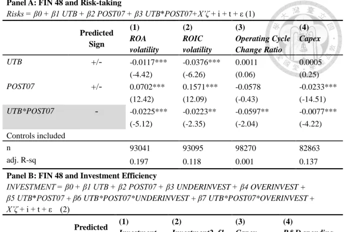
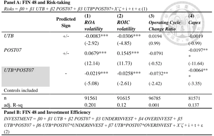
4.3 FIN 48 and Risk-taking

Table 4 reports the results of estimating equation (1). Column (1) and (2) show similar outcomes. The significantly positive coefficient of POST07 indicates that overall economic conditions get more dynamic after 2007 given the global financial

crisis in 2008 and European debt crisis. To specifically capture the effect of how FIN 48 affects firms’ risking-taking, the significantly negative coefficients on

UTB*POST07 confirm it. In the regression with ROA volatility as the dependent

variable (column 1), the coefficient on UTB*POST07 is -0.0207 ( t-stat = -4.75, p

<0.01), suggesting that firms with UTB inherent reduce their risk-taking in the FIN 48 regime relative to other firms in the same industry. The economic significance is such that the reduction is 29% of the mean value of ROA volatility. In column (2), where I use ROIC volatility as the dependent variable, the estimate is less strong but still significant compared to that in column (1). The coefficient is -0.0176 ( t-stat = -1.86, p <0.1), meaning 11% reduction of the mean value of ROIC volatility.

Column (3) and (4) show how firms respond to FIN 48 by changing operational arrangements. They both have significantly negative coefficients on UTB*POST07.

Firms with UTB inherent accelerate their operating cycles by 6.3% and scales down their net capital expenditure over total assets by 0.73% in the FIN 48 regime. The coefficients on UTB*POST07 in Column (1) to (4) all reflect significant negative

risk-taking in the FIN 48 regime.

When it comes to the control variables, LEV, DEP_PUREAC, and STDINVEST are significantly positively for column (1) and (2). It shows that higher levels of leverage, more aggressive choices of accounting methods, and historic operating volatilities will bring about greater firms’ future overall risk-taking. These effects are not obvious for column (3) and (4). I reckon that Operating Cycle Change Ratio and

Capex are more specific aspects of firms’ risk-taking unlike the aggregate level

represented by ROA volatility and ROIC volatility. From LOGAGE, I find that firms reduce their risk-taking as they mature. Last, the negative effect of LOGOPCYCLE contradicts my expectation but I suppose it will not harm the regression results because of the little economic impacts.

Table 4

FIN 48 and Risk-taking

Risks = β

0

+ β

1

UTB + β

2

POST07 + β

3

UTB*POST07+X’ζ + i + t + ε (1) Predicted

Sign

(1) ROA volatility

(2) ROIC volatility

(3)

Operating Cycle Change Ratio

(4) Capex

UTB

+/

-

-0.0119*** -0.0376*** 0.0050 0.0004

(-4.51) (-6.32) (0.26) (0.24)

POST07

+/

-

^{0.0555*** 0.1099*** -0.0583} -0.0234***

(10.68) (10.79) (-0.44) (-14.70)

UTB*POST07 -

-0.0207*** -0.0176* -0.0633** -0.0073***

(-4.75) (-1.86) (-2.17) (-4.03)

LEV

+ 0.0165** 0.0730*** -0.0108 0.0002

(2.43) (4.77) (-0.37) (0.12)

DEP_PUREAC

+ 0.0548*** 0.1045*** 0.0737 0.0026

(4.40) (4.22) (1.32) (0.73)

LOGAGE -

-0.0079*** -0.0232*** -0.0080 -0.0080***

(-4.13) (-5.81) (-0.91) (-13.06)

MTB

+ -0.0019*** -0.0039*** -0.0016 0.0005***

(-6.37) (-4.99) (-1.04) (6.84)

LOGMVE

+ -0.0161*** -0.0324*** -0.0023 0.0035***

(-21.59) (-23.54) (-0.77) (19.56)

STDSALES

+ 0.0009 0.0055 0.0079 -0.0007

(0.24) (0.91) (0.62) (-1.22)

STDINVEST

+ 0.1000*** 0.1480*** 0.0113 0.0013

(11.93) (11.25) (0.53) (1.31)

LOGOPCYCLE

+ -0.0343*** -0.0454*** -0.0037***

(-13.99) (-11.58) (-9.55)

PERFDAROA

+ -0.0043*** -0.0045** -0.0021 0.0006***

(-3.27) (-2.17) (-0.50) (3.36)

_cons 0.2532*** 0.4022*** 0.1498 0.0764***

(15.11) (11.88) (1.22) (12.48)

Year Fixed-Effect Yes Yes Yes Yes

Industry Fixed-Effect

Yes Yes Yes Yes

Std. Error

Clustered by Firm

Yes Yes Yes Yes

n 94443 94497 99678 84031

adj. R² 0.199 0.119 0.001 0.137

t statistics in brackets * p<0.1 ** p<0.05 *** p<0.01

a See Appendix A for variable definitions

4.4 FIN 48 and Investment Efficiency

In my second analysis, I study the relation between FIN 48 and investment efficiency. Table 5 reports the results of regressing equation (2) which is designed to test my second hypothesis. Consistent with my expectations, column (1) to (4) provide evidence that firms with UTB inherent and a greater likelihood of underinvestment (overinvestment) invest more (less) in the FIN 48 regime. The estimated coefficient on UTB*POST07*UNDERINVEST is statistically positive in column (1) to (3). They are 0.0152 for Investment_latf1 ( t-stat = 2.31, p <0.05),

0.0236 for Investment2_f1 ( t-stat = 3.57, p <0.01), and 0.016 for Capex ( t-stat = 7.56, p <0.01). But the coefficient for R&D spending is 0.0061 ( t-stat = 0.92) and not significant in statistical levels. The coefficient on UTB*POST07*OVERINVEST is statistically negative in column (1) to (4). They are -0.0911 for Investment_latf1 ( t-stat = -4.53, p <0.01), -0.1122 for Investment2_f1 ( t-stat = -6.66, p <0.01), -0.0516 for Capex ( t-stat = -9.14, p <0.01), and -0.0416 for R&D spending ( t-stat = -2.61, p

<0.01).

Regarding economic significance, firms with UTB inherently increase

INVESTMENT by 9.44%, 18.3%, 27.6%, and 8.97% of the mean value of

INVESTMENT respectively in column (1) to (4) if they are the firms in the group of

UNDERINVEST. Regarding economic significance, firms with UTB inherently

decrease INVESTMENT by 56.6%, 87%, 89%, and 61.2% of the mean value of

INVESTMENT respectively in column (1) to (4) if they are the firms in the group of

OVERINVEST.

About the coefficients of the control variables, I have a few observations. Being significant negative, the coefficients of LOGAGE indicate that firms invest less as they develop more maturely. The results of LOGMVE seem to reflect similar tendencies that companies’ investment proportions decline when their sizes become larger. MTB, proxy for investment opportunities, are positively related with all four investment variables.