應用密度函數估計提昇小樣本數機器學習之正確度

行政院國家科學委員會專題研究計畫 成果報告

應用密度函數估計提昇小樣本數機器學習之正確度

中 華 民 國 92 年 10 月 29 日

行政院國家科學委員會專題研究計畫成果報告

應用密度函數估計提昇小樣本數機器學習之正確度

Using Density Estimation as An Assistance to Improve the Learning

Accuracy in Machine Learning

計畫編號：NSC91-2213-E006-130 執行期限：91 年 8 月 1 日至 92 年 7 月 31 日

主持人：利德江 成大工管系 教授

執行機構及單位名稱：國立成功大學工業管理科學系(所)

Abstract

This paper is devoted to learn knowledge with a small data set using

statistical learning theory. Since fewer

exemplars usually lead to a lower learning accuracy, many approaches use a big number of exemplars in learning process for higher learning accuracies. However, the idea would be inappropriate when a research is limited by cost and time. To overcome this difficulty, this research uses kernel

methods of Density Estimation to

improve the small size learning. Furthermore, Virtual Samples Generation with Intervalized Kernel Density Estimation is proposed to produce enough information for learning. The provided example shows that this is an economical and efficient method of knowledge acquisition from small data sets. 摘要 本研究針對小樣本的學習問題上採用統 計學習理論來解決。由於樣本數的不足， 所能提供的學習資訊相對的減少，連帶的 學習正確率也會偏低。然而在成本考量 下，此一情況是很難避免的。因此，我們 採用密度函數估計法來找尋小樣本所隱 含的母體資訊，透過密度函數的估計式可 以模擬與原始樣本較接近的虛擬樣本，利 用這些虛擬樣本來作機器學習，將可以得 到較佳的學習正確率。

Keywords: Density Estimation, Intervalization, Kernel Density Estimator, Neural Network, Scheduling, Small-data-set Learning, Virtual Sample Generation.

1. Introduction

The size of training samples is always a key factor in determining a learning machine’s capability of knowledge acquisition. Most of researchers spend a lot of money and time on gathering a big number of data for the learning, because a small data set resulted from limited cost would usually lead to a lower accuracy. Facing this situation, statistical learning theories can help to deal with this problem

systematically. The Small Sample Statistic constituting advanced subjects can contribute significantly in finding statistical learning theories. Besides, Density Estimation is useful to formulate a learning model too.

The research aims at using statistical learning theory to improve a low-accuracy learning resulting from a small data set. Density Estimation, one of the three main parts in statistical learning theory, is the proposed approach as the basis to deal with the small sample size cases. In various methods concerning Density Estimation, we try to refine the form of kernel estimates for suitable small sample case and do learning with the refinement of kernel methods.

There are several assumptions stated to limit the scope of the problem. First, all data used in this study are determinate without noise so that can be treated as exemplars. Second, the data types are all numeric rather than nominal but can be either in discrete or continuous form. The example at Chapter IV will illustrate only the processes with low-dimension variables. Nevertheless, the general form of n-dimension can be derived in the same way.

2. Literature Reviews

It is an intuitive perception that more data usually provide more information for a training task, and can make a learning machine gain higher accuracy. However, there should be an efficient way to use samples instead of exhausting the data set .

Gu et al (2001) presented a statistical approach which is able to find such a right sample size efficiently, called Statistical Optimal Sample Size (SOSS), in the sense that a sample of SOSS sufficiently resembles the entire data. In the SOSS approach, they at first define the sample quality Q, a decreasing function of the averaged information divergence, which is a measure of the difference between SOSS and the entire sample. Given a large data set D, its SOSS is the size at which its Q sufficiently approaches the one computed from the entire sample. The way to search SOSS is an iterative algorithm with acceptable quality pre-set by researchers.

One has been taught that, in traditional statistics, when testing a null hypothesis H , the sample size should 0 be determined at first so that the test has a stated amount of power at a certain alternative hypothesis Ha . The

unknown sample size, necessary at the least, can be found by considering the power of the test at H as a function of a

sample size. In real cases, difficulty exists that the true distribution of the test

statistic under Ha is unknown.

Amaratunga (1999) proposed a searching algorithm, QuickSize, an automated searching procedure that uses computer simulation to find a right sample size. This algorithm involves much trial-and-error and heavy computing before an acceptable sample size with the highest power function value at a given significant level α is found.

Unlike QuickSize algorithm to find a

suitable sample size, Hernandez-Agurirre et al (2002)

proposed a new Sample Complexity Bound for learning. This lower bound is used specially for function learning tasks through neural networks. Sample Complexity Bound means a number of samples needed at least for a learning machine with an acceptable accuracy.

Although many papers study about learning from exemplars, few ones focus on the problem of learning from small sample size. Still several researchers provided ideas and are devoted to the scenario in this problem.

The first kind of scenarios is Virtual

Data Generation, most used in Pattern

Recognition. Niyogi et al (1998) used prior knowledge obtained from the given small training set to create virtual examples in pattern recognition. The idea is that given a 3-D view of an object, a new view from any other

directions can be generated through a lot of mathematical transformations. Samples generated through those new views are so-called virtual samples. That is, there are lots of virtual samples corresponding to every sample so that a learning machine can verify a sample more precisely. Niyogi et al proved that the process of creating virtual samples is mathematically equivalent to incorporate prior knowledge. To create virtual samples may not be the best way to increase the accuracy of learning from small data set but is worth to be pointed out the importance of using prior knowledge from given data.

In continuous data, Chen (2000) proposed a method that used Functional

Virtual Population to create more

samples for training. The idea is to expand the domain of each attribute or variable in a small data set and select possible values from each expanded domain randomly to form a new virtual sample set. The expanding direction depends on data decreasing or increasing. Chen suggested four policies for domains expanding: 1 increasing, 2 decreasing, 3 absolutely increasing, 4 mixed. Yet, to decide which policy is the best choice would be a process of trial-and-error and no theoretical proof was provided to support it.

In Experimental Design, orthogonal data make the small sample more efficiency. Lanouette et al (1999)

thought that designed data sets are more suitable than randomly selected ones due to their higher orthogonality when using small experimental data sets. However, in experimental design, it is sometimes impossible to use a big number of samples to conduct any destructive experiments. Besides, learning is quite different from an experiment; Data sets are always given before learning while experiments gather data after design.

Bayesian Network uses the prior knowledge in sufficient basis of conditional probability distribution of data in the learning; but, small data set still leads Bayesian Network to a poor performance. Onisko et al (2001) proposed a method that uses Noisy-OR gates to reduce the data requirement. The use of Noisy-OR gate is really a scenario for dealing with small sample cases in approximating the conditional probability distribution. But, when independence of variables makes computation easier, the assumption of independence causes variables limiting its capability. Strictly speaking, Bayesian Network can be applied to nominal data rather than numeric data.

2.1 Density Estimation

Density Estimation is one issue of the Satistical Laraning Theory. The purpose of learning is to find any possible model presented in any type to estimate a target value, and statistical

learning is to define any real-value function for the distances between the estimates and target values, or errors. The function is called as a “loss function”, and an expected loss function is considered to be a risk function. The statistical learning problems thus can be treated as problems of minimizing risk functions.

The computation of a loss function need a set of independent and identically distributed samples, such as sets of observations obtained from a series of experiments, trials, or experiences. This kind of samples is so-called empirical data. Therefore, to minimize the learning risk means to minimize the risk function of empirical data. It is the Empirical Risk Minimization (ERM) principle that defines a learning process for any given set of observations.

Density Estimation is used to estimate the actual probability density function on the basis of a limited number of examples. It provides an alternative to find the underlying density function of a given dataset while no functional form is assumed.

The common approaches of Density estimation include including the Naive Estimator, Kernel Methods, Series Methods, Maximum Penalized Likelihood Estimator, and the Artificial Neural Network based method. However, most of them can find good estimators

only in the large data cases. L k x h xk+ h xk− L Re la ti ve F re qu enc y th e k th b in 1 x X 0 0 0 .1 0 .2 0 .3 ( k) f x L L h

Figure 2.1. A histogram has the same bandwidth in each bin.

2.1.1 Histograms and the Naive Estimator

The histogram is the oldest and widely used method for Density Estimation. It provides the original information about a dataset. Given a set of observations with size n, { ,x1L,xn},

and a bandwidth (bin width) h , according to Figure 2.1 the probability of observations within an interval

(x_k−h x, _k+h) could be 2h×f x( _k), where

( )

f • is a frequency function and k is any integer from {1,_L, }n . That is, the probability concerned with the observations is equal to the area of corresponding rectangle, or said “bin”, as the following:

( _{k k} ) 2 ( _k)

P x − <h X <x +h = h× f x . Mathematically, a density function, f ,

is presented as the general form: 0 1 ( ) lim 2 h f x h → = P x( − <h X < + . x h) Since f x( ) is an unknown density function underlying the observations, we can estimate the probability

( )

P x− <h X < +x h with the proportion of the samples falling in (x−h x, +h). The naive estimator of a density function can be derived as Function (1) by selecting a bandwidth h . To express the naive estimator more concisely, an indicator function w( )• can be employed as in Function (2) and (3).

Function (3) is suggested by M. Rosenblatt (1956), named the Rosenblatt estimator. The property of a naive estimator or the Rosenblatt estimator can be checked from any histogram such as that in Figure 2.1. Each bin has the same width h, and the type of f xˆ ( ) is a step function, which is step-wise. Although a naive estimator can present the information easily, f xˆ ( ) is still not a continuous function for having jumps at points {X_i ±h}. We believe that a true population should contain enough data to construct a more smooth and continuous density function even though the obtained observations in hand are of a small sample size.

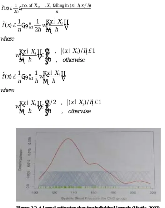
Figure 2.2. A kernel estimator showing individual kernels (Hastie, 2002).

2.1.2 Kernel Methods

The naive estimator or the Rosenblatt estimator is usually quite rough. A continuous, differentiable function, K( )• , is considered to substitute for the indicator function,

( )

w• . The K( )• , called “a kernel function”, counts observations close to

i

X with weights that decrease with the distance from Xi.(4)

Parzen (1962) proposed the smoothing kernel estimator, Function (4), called the Parzen’s estimator; and the bandwidth h has a name here, the smoothing parameter. Besides, the unknown density f has continuous derivates of all orders required. Figure

1 no. of X , , falling in ( , ) 1 ˆ ( ) 2 n X x h x h f x h n − + = × L ₍₁₎ 1 1 1 ˆ ( ) 2 n i i x X f x w n = h h −   = ×Σ _{ }   (2) where 1 , ( ) / 1 0 , i i x X h x X w h otherwise  − < −   _{ = }    _{ } 1 1 1 ˆ ( ) n i i x X f x w n = h h −   = ×Σ _{ }   (3) where 1/ 2 , ( ) / 1 0 , i i x X h x X w h otherwise  − < −   _{ = }    _{ } 1 1 1 ˆ ( ) n i i x X f x K n = h h −   = Σ _{ }   (4)

2.2 presents the shape of a kernel estimator showing individual kernels.

Consistency and convergent properties are the reasons why the kernel method is widely used. The probability of yielding errors in estimating would approach to zero and the estimate would converge to the true density function in large sample cases.

In most applications of kernel density estimator, K( )• is often a symmetric function such as the Gaussian function. It makes kernel estimator suffer from a drawback when applying to asymmetrically distributed data. Another disadvantage is the constant smoothing parameter across the entire sample.

2.1.3 Series Methods and Maximum Penalized Likelihood Estimators

The orthogonal series estimator was first presented by Watson (1969) to deal with density estimation problems. Fourier series are developed to represent any function using sine and cosine curves, especially for cycle functions. Here, the employment of orthogonal series method is to estimate density function by estimating the coefficients of its Fourier expansion.

Maximum likelihood (ML) method has been used in parametric Density Estimation before de Montricher et al

(1975) used it in nonparametric Density Estimation from a viewpoint of penalty. The ML method is a widely-used technique, however, the maximal value of likelihood function does not always exist. Tapia (1978) made the first appearance of Maximum Penalized Likelihood (MPL) method after De Montricher proposed the penalty idea. The penalty is quantified using a function, which measures the discrepancy between the estimator and the true density, called roughness penalty.

2.1.4 Neural Network Based Methods

The application of Artificial Neural Networks (ANNs) speeds up the development of methodology in Density Estimation. It is really a very way to find the parameter of a determinate density. A prediction model formed by regression or time series is a common example, called the conditional density, which uses given data of independent variables to model the density of dependent variables. For another example, Williams (1996) used the output of a neural network to estimate the parameters of a density model including multivariate and univariate cases, and showed the performance was as fine as that of traditional methods. In Husmeier and Taylor’s method (1998), they considered a Gaussian Mixture model for predicting the mean and variance of conditional densities with using a

two-hidden-layer structure. They believed that two hidden layers would be better than one for predicting conditional distribution (1997). Since their second hidden layer is a Gaussian kernel layer, it is clear that, the structure assumes the input data are normally distributed. That is, the applications of parametric methods still suffer from the drawback of being unable to deal with unknown density cases.

Neural network based methods can also be applied to nonparametric approaches. In Schioler and Kulczycki’s investigation (1997, 1998), a neural network structure, on the basis of kernel methods, has been set up for estimating conditional distributions and their associated quantiles. The neurons in the network structure are defined from a kernel function and the size equals to the number of data. Note that, however, the smoothing process is necessary after using kernel methods in a neural network way.

Miller and Horn (1998) proposed an algorithm on the basis of entropy maximization, closely related to Maximum Likelihood Methods. According to their research, in neural network structure, the maximal entropy can be achieved by using gradient ascent way. It consists of two steps: Encoding step provides an estimate of the probability density, and Decoding step produces an ensemble of data with the

desired distribution.

The applications of Neural Network need a large number of data to train for a stable result. There must be a lot of nodes in the network structure and many connected weights that need to be trained. If each weight stands for a parameter, it is impossible to train a network steadily by putting samples fewer than the number of weights. From the viewpoint of statistics, sample size less than the number of parameters always leads to an under-estimated situation. Consequently, using Neural Network may not be the best way to do Density Estimation with small sized samples size.

3. Virtual Sampes Generation

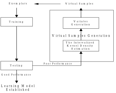
The reason for the poor learning from small data sets is its lack of information about the population. As mentioned above, it is necessary to sample a big number of data in an unstable process for covering all possible situations. That is, the current data are unrepresentative. Virtual Samples Generation (VSG) is a direct way to overcome this difficulty. It contains 2 steps in our study, shown in Figure 3.1, step 1: The Intervalized Kernel Density Estimation, and step 2: Variates Generation. The current data provide prior information about its distribution. We incorporate the prior information in formulating the

V i r t u a l S a m p l e s G e n e r a t i o n T r a i n i n g T e s t i n g T h e I n t e r v a l i z e d K e r n e l D e n s i t y E s t i m a t i o n V a r i a t e s G e n e r a t i o n V i r t u a l S a m p l e s E x e m p l a r s G o o d P e r f o r m a n c e P o o r P e r f o r m a n c e L e a r n i n g M o d e l E s t a b l i s h e d

Figure 3.1 Virtual Sample Generation in the learning process contains two steps : the Intervalized Kernel Density Estimation step and the Variates Generation step.

intervalized kernel density estimator and generate the virtual samples for learning.

3.1 The Intervalized Kernel Density Estimation

Mathematically, small sample size learning cannot achieve high accuracies no matter what kind of learning machine is employed. To overcome it, we believe that realizing data behavior could make the size problem less influential. For instance, if we have understood a small sample possessed a normal distribution, we could generate more data from the normal density function for learning. Therefore, Density Estimation is thought an effective approach to lift up the accuracy in small sample learning. Along with the conceptual strategy, a special technique---Intervalization is proposed to improve the estimation task.

The concept of intevalization is

developed on the basis of Kernel

Density Estimation methods. There are a

lot of kernel functions for choices, such as Epanechnikov, Biweight, Triangular, Gaussian, Rectangular etc. Although Kendall and Stuart (1973) found that Epanechnikov kernel function has a remarkable efficiency than others, we will use the most common one--- Gaussian kernel function (Function (5)) for the choice of kernel functions is not the key point in our study. It makes the density estimator look smooth and can simply interface with computer graphic works (i.e. Mathematica 4.0).

2 2 1 , ( , ) 2 t e t π − ∈ −∞ ∞ (5)

3.1.1 Intervalization in Small Sample Sets

One of the problems in small sample learning using Density Estimation is

(a) classinterval 1,= h=0.5 (b) classinterval 5,= h=2.5

Figure 3.2(a)(b). Directly using kernel methods can lead to a poor estimate.

(a) classinterval 1=

(b) classinterval=2, h=1 (c) classinterval=2, h′=1 classinterval=5, h′′=2.5

Figure 3.3. (a) is the histogram of 10 data with class interval equal to 1. (c) with varied smoothing parameters that fit well than the fixed ones of (b).

about the rough estimate. Figure 3.2 shows how poor an estimate is resulted from few samples. In Figure 3.2(a), the twin-modal curve is an estimate, by kernel methods, of the underlying density using six samples. The original data were classed into 4 bines. If all the six samples belong to 1 bin like that in Figure 3.2(b), the uni-modal curve can be the estimate. Intervalization means the process to shrink the number of bines. Since we have too little message about these six samples to believe that

they are distributed as a multi-modal distribution, the basic concept of intervalization is to create more information from data to determine the underlying distribution. In fact, the process of intervalizing the data is done on the basis of kernel methods, and the final number of bins is not a constant. Just like the twin-modal curve in Figure 3.2(a), if these two peaks are located very close, the original data could be distributed as a uni-modal density, such as Figure 3.2(b). On the contrary, if

L L L

I n te r v a liz in g

1 b in 1 0 0 b in s

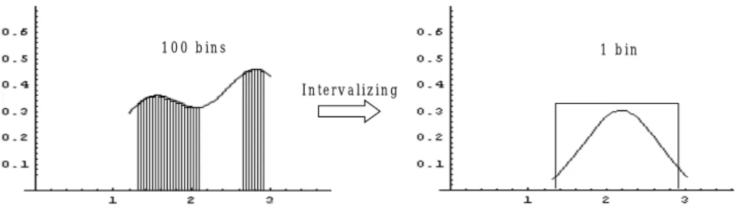
Figure 3.4. Intervalization may lead to the irrationalism in large samples.

peaks are located far apart from each other, the density might have the shape of multi-modal. For detailed explanation, consider another example that Figure 3.3(a) is a histogram of 10 data with class interval equal to 1. Since the six data of them on the left are located so close that they can be distributed in a uni-modal density after enlarging the class interval from 1 to 2 (Figure 3.3(b)), or from 1 to 5 (Figure 3.3(c)). Consequently, the point reveals that the ordinary kernel estimator, Function (4), counts on a smoothing parameter h whereas the intervalized kernel estimator concentrates on the determining of the bin number and the scale of class interval. Although h and the scale of class interval have a proportional relationship, they make different influences to the ordinary and intervalized kernel estimators.

In Figure 3.3(b)(c), the h or h′ is fixed across the left six samples so the ordinary estimator can work well. However, in Figure 3.3(b), the drawback of the ordinary estimator appears while the data are widely distributed and the intervalized one (Figure 3.3(c)) looks

more reasonable. In other words, intervalization provides a mechanism for choosing the number of bins, which can have various sizes.

For example, in Figure 3.4, suppose we have thousands of data available and are classified into 100 bins in a density estimate. The curve looks awkward. Note that when we intervalize the data set to 1 bin and have another density estimate, the irrationalism appears immediately from the histogram. In the example, intervalization eliminates the multi-modal shape of the original data.

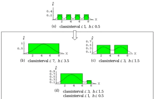
In another extreme situation, for example, that 4 data in hand are distributed as shown in Figure 3.5. Kernel methods cannot perform well by just adjusting the smoothing parameter h. Generally, it is hardly possible that only these 4 data will form a four-modal density like that in Figure 3.5(a). The estimates after intervalizing (Figure 3.5(b)(c)(d)) seem to be more reasonable. The reason is the size of h must be fixed across the entire sample in ordinary kernel methods whereas the intervalized one can have different h’s.

(a) classinterval 1,= h=0.5

(b) classinterval=7, h=3.5 (c) classinterval=3, h=1.5

(d) _{classinterval=3, h=1.5} classinterval=1, h=0.5

Figure 3.5. (a) The original data has the estimate with four-modal shape. (b) (c)The intervalization of 1 bin and 2 bins. (d) The intervalization with various h.

As shown above, an arbitrary varied smoothing parameter h in the same data can improve this kind of drawback of kernel methods. We try to refine Function (4) to possess the capability of choosing different h in a model. Function (6) is a refinement of ordinary kernel methods, a proposed density estimator with varied smoothing parameter h , named the intervalized _i

kernel estimator. To further describe the estimator assuming there are n data to be intervalized using m different smoothing parameters (i.e. h_i i= L1, ,m), each h _i

is designed to be tied with a number of samples, n_i and a kernel function,

( ) i K • . 1 1 1 1 ˆ ( ) m ni j i j i i i x X f x K n = = h h −   = Σ Σ _{ }   where 1 m i i n= Σ₌n . (6)

The idea of varying h to make it more

sensitive to the data at local bins, and processing intervalization to shrink unnecessary bins (i.e. to increase the size of h) are the main differences between Function (4) and (6). Note that, users can define the value or values of

i

h by themselves. For example, Figure

3.5(b)(c) show a fixed h_i in each model

and (d) shows various h_i.

To illustrate Function (6) in graphs, we express the estimate with the curve in Figure 3.5(d). There are 2 different smoothing parameters and kernel functions, m=2, as the following

2 1 1 3 1 1 1 1 2 1 1 2 1 1 1 ˆ ( ) 4 1 1 1 . 4 i j n i j i i i j j j j x X f x K h h x X x X K K h h h h = = = = −   = Σ Σ _{ }     −   −  = _Σ _{ }+ Σ _{ }      

and (6) is that the intervalized kernel estimator can employ different kernel function like that in the above illustration, K1( )• and K2( )• can be

the same or distinct forms.

3.1.2 The General Form of Intervalized Kernel Density Estimation

Now we expand the intervalized kernel density estimation method from one-dimensional to the general form,

multi-dimension one, in high-dimensional Density Estimation, the situations are always more complicated than that in univariate cases. Let Χ =( ,x1L,xp) be a random vector

with p-dimension, where x1,L,xp are

its variables in every dimension. Before constructing the multivariate density estimator, a discussion of the independence is necessary. Some of

1, , p

x L x can be independent while others can be related. For example, assume Χ is somebody’s health and

1

x is his age, x2 is his weight, x3 is

the index of coronary heart disease, and

4

x is his height etc. We may claim that

3

x can be related to x1 or x2 and have

nothing to do with x4. In other words,

all the dimensional variables, xi, can be

partially independent or partially dependent in multivariate data set.

Therefore, the multivariate density estimator is the product of independent and dependent vector’s density estimator, where independent vector ΧI has

mutually independent elements, x1,L,xk,

and dependent vector ΧD has

correlated elements, xk+1,L,xp, such as

in Function (7).

Since x1,L,xk are mutually

independent variables, the estimator of the joint density function, g xˆ ( ,1 L,xk),

can be expressed by 1 ˆ ( , , _k) g x _L x f xˆ ( )_{1 1} ⊥ = _Lf xˆ ( )_{k k} 1ˆ ( ) k t= f xt t = Π (8) where ˆ t

f is the uni-variate intervalized kernel estimator, Function (4). Verbally, the multivariate estimator is the multiple product of every univariate estimator in the cases of independent variables. ˆ ( ) f Χ =gˆ (Χ_I)lˆ(Χ _D) where Χ = Χ Χ( _I, _D), 1 ( , , ) I x xk Χ = _L , Χ =_D (x_k+1,_L,x_p)

gˆ (Χ_I) =g xˆ ( ,_{1 L},x_k), the estimator of joint density

g x( ,_{1 L},x_k);

ˆ(l Χ_D)=l xˆ( _k+1,_L,x_p), the estimator of joint density 1

( _k , , _p)

l x _{+ L} x .

And we construct the multivariate kernel density estimator from the original kernel estimator while

1, ,

k p

x+ L x are correlated with each other.

The original multivariate kernel density estimator, defined by Parzen (1962),

with kernel function K( )• and smoothing parameter vector p

h in

p-dimension (i.e. p

h is on _ℜp

) is set as Function (9). For the computational and smoothing considerations, p

h is a

constant vector (i.e. _hp ₌( ,_h , )_h

L ). That 1 ˆ ( k , , p) f x ₊ L x = fˆ (Χ =D) 1 1 n D i i p X K nh = h Χ −   Σ _{ }   where Χ =D (xk+1,L,xp), ( , , ) p h = h_L h , 1, , k p x_{+ L} x are correlated. (9) 1 ˆ( k , , p) l x ₊ L x = Χ =lˆ( D) 1 1 1 m n 1 D j i j p i i i X K n = = h h Χ −   Σ Σ _{ }   where Χ =D (xk+1,L,xp), ( , , ) p i i i h = h _L h , m i i n= Σ n 1, , k p x _{+ L} x are correlated. (10) ˆ ( ) f Χ =gˆ (Χ_I)lˆ(Χ _D) where Χ = Χ Χ( I, D), 1 ( , , ) I x xk Χ = _L , Χ =_D (x_k+1,_L,x_p) 1, , k

x _L x are mutually independent,

x_k+1,_L,x_p are correlated.

gˆ (Χ_I) =g xˆ ( ,_{1 L},x_k)= Πk_t=1f xˆ ( )_{t t} ,

the estimator of joint density g x( ,_{1 L},x_k),

(11) ˆ ( ) 1 m₁ ni₁ 1 t t j t i j i i i x X f x K n = = h h −   = Σ Σ _{ }  ,

the estimator of density f x , ( )t

ˆ(l Χ_D)=l xˆ( _k+1,_L,x_p) 1 m₁ n ₁ 1 D j i j p i i i X K n = = h h Χ −   = Σ Σ _{ }  ,

the estimator of joint density l x( k+1,L,xp).

hip =( ,hi L, )hi ,

m₁ i i n= Σ₌n .

means each high-dimension bin has the same bin-width, h.

Like the intervalization in univariate cases, we have to consider the multivariate cases with small sample size. It is hard to show by graphs the densities and histograms in high dimension. Nevertheless, intervalization in high dimension can be considered as that the closer observations are bounded within a unimodal hypersurface, which is expressed in a density-like function. For example, with a small sample size in 2-dimension, if the observations scatter closely, we should favor that there is a unimodal surface sheltering the present data even though they are not in the same bin. On the contrast, the data would possess a multi-modal density if they were distributed widely.

On the basis of intervalization, a refinement of Function (9), which possesses m different smoothing

parameter vectors p i h and kernel functions Ki( )• , ( p i h , Ki( )• ), would

be suitable for (or corresponding to) ni

observations. Then, Function (10) is the intervalized multivariate kernel density estimator of correlated variables,

1, ,

k p

x_{+ L} x .

The complete general form of the intervalized multivariate kernel estimator can be found by combining Function (8) and Function (10). Suppose

1

( ,x ,xp)

Χ = _L is a data vector in

p-dimension for a observation and its

elements are divided into two parts: mutually independent variables vector

1 ( ,x1 ,xk)

Χ = _L , and correlated variable vector Χ =2 (xk+1,L,xp). Function (11) is

the complete general form of an intervalized multivariate kernel density estimator.

3.2 Variates Generation

Random Variate Generation has an inverse process comparing with that of Density Estimation. As mentioned before, Density Estimation estimates the underlying density or guesses the true distribution of a given data set whereas Random Variate Generation produces a desired number of samples from a determined density. Simulation is still a useful approach in Random Variate Generation. Such as Markov Chain Monte Carlo Method, it is used widely for generating a random vector millions of times to obtain statistically reliable results. Besides, some methods generate variates from certain distributions, like the Polar method for generating normal random variables (Ross, 1996).

However, most of these methods are only suitable for specific, well-defined distributions. They can hardly be applied to an arbitrary density. In our study, most density estimates have more complicated forms than usual random variables do. Therefore, applying the inversion method seems to be a more

direct way.

4. The Experimental Study

The experimental data is an example from a flexible manufacturing system (Chen, 2000). There are four variables in this case, where X₁ represents the buffer size, X2 represents the arrival rate of parts, X represents the speed 3 of automobile general motors, and Y is

the coding number of the best scheduling rule. We re-code these three scheduling rules: FCFS means the rule of “First come, first served” coded as 1, SPT means the rule of Short Processing Time coded as 2, and EDD means the rule of Earlier Due Date coded as 3. We try to learn a concept from the training data to predict the best scheduling rule.

This data set contains a small data set of 40 row-data form the FMS. First, we separate the data into two groups: half of them are the training set and the rest are for testing. Second, a BPN,

Pythia version 1.02, featuring

back-propagation networks, is employed as the learning machine. Pythia has a special function --- Evolutionary Optimizer --- a tool for searching appropriate network structures based on the training data set through the Genetic Algorithm (GA).

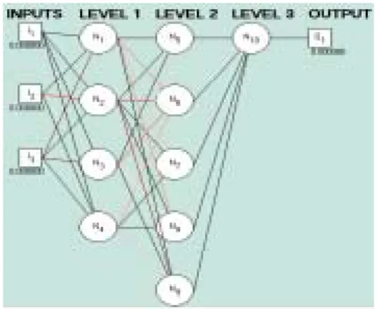
A 3-4-5-1-network structure is generated by the searching mechanism. It represents a four-layer structure,

where 3 is the number of neurons in the input layer, and 4,5,1 are those neurons in hidden layers, respectively. Figure 4.1 is the diagram of a 3-4-5-1 network. To confirm the appropriateness of this structure, we use it to classify the training data set. The average correct rate is 95%, that is, the 3-4-5-1 structure can represent the training data set with only 5% error.

Figure 4.1 A 3-4-5-1 network structure generated by GA searching mechanism.

Because the training data size is too small (only 20 data) to cover all possible situations, the average testing accuracy of 10 trials is 29.77%, meaning a poor performance. The testing results are shown in Table 4.1.

Table 4.1 The testing accuracies are very poor.

No. of trial The accuracy of classifying the 20 testing data 1 0.3 2 0.3 3 0.45 4 0.25 5 0.3 6 0.35

7 0.35 8 0.35 9 0.325 10 0.3

Average 0.2977

4.1 Virtual Samples Generation

The experiment has two works: 1. Virtual Samples Generation and 2. Learning scheduling knowledge, when applying the Virtual Samples Generation to improve the learning in the scheduling data.

4.1.1 The Intervalized Kernel Density Estimation

Now we use the Intervalized Kernel Density Estimation method (Function (11)) to find the approximate density estimators of the current data. There are 3 independent variables, X₁ X₂ and

3

X , and 1 class variable, Y. Therefore,

the joint probability density estimators for each class is the conditional joint probability density estimators,

1 2 3

ˆ ( , , | )

f x x x Y =y where y=1, 2, 3 . On assuming X₁ X₂ and X₃ be mutually

independent, the conditional joint probability density estimator can factor into 3 independent probability density estimators: f x Yˆ ( |1 = y) , f xˆ ( |2 Y =y)

and f xˆ ( |3 Y= y). Thus, Function (6) can

deal with these uni-variate cases sufficiently.

4.1.2 Variates Generation

Following the intervalized kernel density estimation, variates generation is the second step in virtual samples generation. We can apply any kind of generation approach to produce the desired samples. And since we have assumed the independence between these three variables, respective discussions for each variable in each class can simplify the processes of variates generation. For testing more precisely, we get several virtual sample sets by redoing the generation process for three time, namely set 1st, 2nd, and

3rd respectively.

4.2 Learning with the Virtual Samples

For verifying the improvement of learning from small data sets by the virtual samples generation step, we applying the virtual training data to the same structure of BPN shown in Figure 4.1. If the virtual samples work, the learning accuracy would vary with the new knowledge.

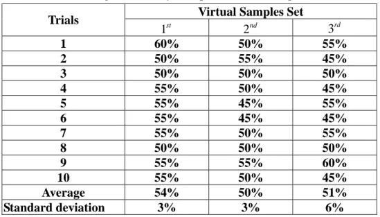
We use the three virtual samples sets to train the network structure and obtain the learning accuracies of the same testing data set, respectively. The observed accuracies from 10 trials are list in Table 4.2. Learning from the first virtual samples set seemingly performs better than the others.

Table 4.2 The learning accuracies by three possible virtual samples with 10 trials.

Virtual Samples Set Trials 1st 2nd 3rd 1 60% 50% 55% 2 50% 55% 45% 3 50% 50% 50% 4 55% 50% 45% 5 55% 45% 55% 6 55% 45% 45% 7 55% 50% 55% 8 50% 50% 50% 9 55% 55% 60% 10 55% 50% 45% Average 54% 50% 51% Standard deviation 3% 3% 6%

The experiment study is concerned with verifying the performance of improving the small data sets learning through the virtual samples generation. We choose a set of scheduling data consisting of only 40 exemplars for the experiment. The difference between the training and testing data are so significant that the average learning accuracies is poor (29.77%). However, we try to gather more information about the 20 training data with formulating the intervalized kernel density estimators and then generate more data as the virtual training sets. These extra information help classify the best scheduling rules of the testing data, therefore, the learning accuracies of the virtual training sets increase to 50%-54%. In other words, the virtual samples generation with the intervalized kernel density estimation helps for improving the poor learning from small data sets.

5. Disscussion

Virtual Samples Generation with the Intervalized Kernel Density Estimation overcomes the difficulty of learning with insufficient data. We believe that generating more samples resembling in the small training sets makes the learning perform well. And we explore the true distributions of data with the proposed intervalized kernel density estimation for samples generation.

The setting of h should be based on

the users’ background knowledge. That is, a scheduling engineer can have long been familiar with the distribution of

1 2 3

(X ,X ,X |Y =y) and do a better setting than us. Besides, we suggest a referable parameter --- the standard deviation, ˆs. In Class 1, a only-one-datum case, if we ignore the standard deviation of

1| 1

X Y = , X2|Y =1, and X3|Y=1, we

might select the same smoothing parameter for f x Yˆ ( |1 =1), f xˆ ( |2 Y =1),

and f xˆ ( |3 Y =1). For example, suppose 1

h= is set for f x Yˆ ( |1 =1), f xˆ ( |2 Y=1),

and f xˆ ( |3 Y =1), the generated variates

might located around the point

1 2 3

(X ,X ,X |Y=1) =(8, 20, 50 |Y=1) and

the domain of X2|Y =1 and X3|Y =1

would not be found.

When formulating the conditional intervalized kernel density estimator of

1 2 3

(X ,X ,X |Y= y), we have assumed the three variable s are independent of one another for simplifying the works. Nevertheless, the relationship between the variables should be considered as an important factor affecting the quality of virtual data.

Note that we also can generate random vector (X1,X2,X3|Y =y)

without the independent assumption. For example, suppose that (X1,X2|Y =y) is

following a bivariate normal distribution with its mean vector (µ µ1, 2|Y =y) ,

variance vector 2 2

1 2

(σ σ, |Y = y), and the correlation coefficient ρ. That is, there must be a linear relationship between

1|

X Y =y and X2|Y = y according to

the property of bivariate normal distributions. After generating variates of X1|Y =y, we can have variates of

2|

X Y =y through linearly transferring (Function (19)) instead of generating it directly.

In other words, the generation works can be simpler in correlated variables than those in uncorrelated ones. We can have a set of variates of one variable through the transforming relationship with other variables.

Another issue is the size of virtual data. In the scheduling case, we train the BPN network with a part of virtual samples (60 data), not all of them (90 data), after the generation work. We know that all the virtual data are not really sampled from the data population. Figure 5.1 can represent the relationship between the virtual data set and data population.

Data Population

Virtual data Small data set

Figure 5.1 Virtual data always covers part of true data population.

Since we explore the domain of true data by formulating the corresponding intervalized kernel density estimators, the population representation of the virtual data cannot be guaranteed entirely. For this reason, we select randomly partial virtual data for training. 2| 2| 2| 1| 1| 1| ( ) Y y Y y Y y Y y Y y Y y X µ ρσ X µ σ = = = = = = = + − ₍₁₉₎

Reference

陳隆昇, 功能性虛擬母體觀念之發展及其在 機器學習中之應用, 國立成功大學碩士論 文, 民國 89 年

Abu-Mostafa, Y. S. (1993). An Algorithm for Learning from Hints. Proceeding of 1993

International Joint Conference on Neural Networks. 1653-1656.

Ammaratunga, D. (1999). Searching for the Right Sample Size. The American Statistician,

53, 52-55.

Carter, M. A., Oxley, Mark E. (1999). Evaluating the Vapnik-Chervonenkis dimension of artificial neural networks using the Poincare polynomial. Neural Works, 12, 403-408. Carter, M. A. (1995). The mathematics of

measuring capabilities of artificial neural networks, Ph. D. thesis, Air Force Institute

Institute of Technology, Wright-Patterson AFB,

OH. DTIC ADA297408.

Cherkassky, V., Shao, X. (2001). Signal estimation and denoising using VC-theory.

Neural Works, 14, 37-52.

de Montricher, G. M., Tapia, R. A., & Thompson, J. R. (1975). Nonparametric maximum likelihood estimation of probability densities by penalty function methods. Annals of

Statistics 3: 1329-1348.

Hastie, T., Tibshirani, R., & Buja, A. (1999). Flexible Discriminant and Mixture Models.

Statistics and Neural Networks Advances at the Interface-1, J. W. Kay and Titterington

(ed.), 1-23.

Hastie, T., Tibshirani, R., & Friedman, J. (2001).

The Elements of Statistical Learning-Data Mining, Inference, and Prediction. New York:

Speinger-Verlag.

Husmeier, D., Taylor, J. (1997). Predicting conditional probability densities of stationary stochastic time series. Neural Works, 10(3), 479-497.

Husmeier, D., Taylor, J. (1998). Predicting conditional probability densities: Improved training scheme combining EM and RVFL.

Neural Works, 11(1), 89-116.

Kendall, M.G., Stuart A. (1973). The Advanced

Theory of Statistics, Volume 2, 3rd Edition.

London: Griffin.

Kulczycki, P., Schioler, H. (1998). Estimating Conditional Distribution by Neural Networks.

Neural Networks Proceedings, 2, 1344-1349.

Lanouette, R., Thibault, J., & Valade J. L. (1999). Process modeling with neural network using small experimental datasets. Computers and

Chemical Engineering e, 23, 1167-1176.

Niyogi, P., Girosi, F., & Tomaso, P. (1998). Incorporating Prior Information in Machine Learning by Creating Virtual Examples.

Proceeding of the IEEE, 86(11), 275-298.

Miller, G., Horn, D. (1998). Probability Density Estimation Using Entropy Maximization.

Neural Computation,10, 1925-1938.

Minsky, M., Papert, S. (1969). Perceptrons. Cambridge, MA: MIT Press

Mitchell, T. M. (1997). Machine Learning. New York: McGraw-Hill.

Parzen, E. (1962). On estimation of a probability density function and mode. Annals of

Mathematical Statistics, 33, 1065-1076.

Plutowski, M. E. P., Cottrell, G., & White, H. (1995). Experience with Selecting Exemplars from Clean Data. Neural Works, 9, 273-294. Rosenblatt, M. (1956). Remarks on some

nonparametric estimates of a density estimation. Annals of Mathematical Statistics, 27, 832-837.

Ross, S. M. (1996). Simulation/Second Edition. San Diego: Academic Press.

Schioler, H., Kulczycki, P.(1997) Neural Network for Estimating Conditional Distribution. IEEE Transaction on Neural

Networks, 8(5), 1015-1025.

Silverman, B. W. (1990). Density Estimation for

Statistical and Data Analysis. New York:

Chapman and Hall.

Sontag, E. D. (1992). Sigmoids distinguish more efficiently then heavisides. Neural

Commputation, 1, 470-472.

Sontag, E. D. (1992). Feedforward nets for interpolation and classification. Journal of

Computer and System Sciences, 45, 20-48.

Nonparametric Probability Density Estimation. Baltimore: Johns Hopkins

University Press.

Valiant, L. G. (1984). A theory of learnable.

Communication of the Association Computing Machinery, 27, 1134-1142.

Vapnik, V. N. (2000). The nature of Statistical

Learning Theory. New York: Speinger-Verlag.

Vapnik, V. N., Chervonenkis, A. Y. (1971). On the convergence of relative frequencies of events to their probabilities. Theory of

Probability and its Application, 2, 264-280.

Watson, G. S. (1969). Density Estimation by Orthogonal Series. Annals of Mathematical

Statistics, 40, 1496-1498.

Williams, P. M., (1996). Using Neural Networks to Model Conditional Multivariate Densities.

Neural Computation, 8, 843-854.

Yang, H. H., Murata, N., & Amari, S. (1998). Statistical Inference: Learning in Artificial Neural Networks. Trends in Cognitive Science, 2(1), 4-10.