以多種預測法配合變異數提升直方圖式可逆資訊隱藏技術之品質與藏量

全文

(1)國立屏東教育大學資訊科學系碩士論文以多種預測法配合變異數提升直方圖式可逆資訊隱藏技術之品質與藏量. Histogram based reversible information hiding improved by multiple prediction methods with the variance to enhance image quality and capacity 研究生：劉冠良指導教授：楊政興. 博士. 中華民國一百零三年六月.

(2) 以多種預測法配合變異數提升直方圖式可逆資訊隱藏技術之品質與藏量 Histogram based reversible information hiding improved by multiple prediction methods with the variance to enhance image quality and capacity 研究生：劉冠良. Student：Kuan-Liang Liu. 指導教授：楊政興. Advisor：Cheng-Hsing Yang. 國立屏東教育大學資訊科學系碩士論文. A Thesis Submitted to Department of Computer Science College of Sciences National Pingtung University of Education in partial Fulfillment of the Requirements for the Degree of Master in Computer Science June 2014 Pingtung, Taiwan, Republic of China. 中華民國一百零三年六月.

(3) II.

(4) Acknowledgements 轉眼間二年的碩士求學生涯即將結束！在此，冠良有太多人需要感謝，首先最需要感謝的是我的指導教授楊政興博士，在這兩年的研究生活中不辭辛勞的傾囊相授，才能讓此碩士論文得以順利完成。在楊老師的諄諄教誨引導下，冠良不僅在這二年的研究生活中學習到如何去發現問題、獨立思考並且解決問題之能力，更從日常生活中學習到老師的待人處世的道理，甚至有幸能夠有兩次出國參加研討會的經驗，以及在國內多次的研討會，在與會的過程及經歷都讓學生受益良多！此份師恩銘記在心。再者，冠良亦由衷感謝平時的團體 Meeting 老師，林義凱博士與黃樹乾博士，以及碩士論文口試的口試委員，林義凱博士及黃河銓博士，給予我許多的寶貴意見與指教，讓此碩士論文可以更加的充實與完整。此外，還要感謝屏東教大資訊科學系給予學生們如此優良的研究環境，以及系上所有老師的教導與助理的幫助，讓學生們得以順利的完成學業。以及感謝實驗室資科所 102 級的所有同學們與學弟、妹們，在此二年的互相督促與關懷，以及一些默默關心我的朋友們，讓我在屏東教大碩士生涯中留下了難忘的回億。最後，感謝我親愛的父母與家人們全心全意地給予我支持與鼓勵，讓我無後顧之憂的學習並順利的取得碩士學位，僅此以此論文成果獻給他們。. 劉冠良. 謹誌. 中華民國一百零三年六月二十五日. i.

(5) 中文摘要在可逆式資訊隱藏中，預先預測是一個很好的方法可以有效的將機密訊息藏入影像中。在本論文中，我們提出一個可逆式的資訊隱藏基於多種預測方法以及使用變異數的方法。我們的方法中，每一層在藏入機密訊息之前我們會有兩種策略以及四種預測方式。首先，如果我們的目標是高藏量便計算各種預測方式的藏量；另外，如果我們的目標是高品質便計算各種預測方式的效率比以選擇該使用那種預測方式。當確定選擇哪種預測方式之後，基於變異數所算出的門檻值將用來確定那些像素應該加入位移和嵌入。如果該區域複雜度小於門檻值，則像素將參加機密藏入或者位移；反之，則像素不會參與嵌入及位移的過程。因此，某些像素將避免執行位移的過程，這會減少影像的失真。經由實驗結果可以發現我們的藏量及品質都高於其他的研究。. 關鍵詞: 資訊隱藏、可逆式、變異數、影像品質、直方圖。. ii.

(6) Abstract Reversible data hiding based on prediction methods is a good technique that can hide secret bits into cover images efficiently. In this study, we propose a reversible data hiding method based on multiple prediction methods and local complexity. In our proposed method, before we embed the secret message in one level, we evaluate four prediction methods by two ways to decide which prediction method will be used. First, if we want to achieve high-capacity, the prediction methods’ capacities are calculated. Second, if we want to achieve high-quality, the prediction methods’ efficiency ratios are calculated. When the selected prediction method is applied, a threshold based on local complexity is used to determine which pixel should join the shifting and embedding process. If the local complexity is smaller than the threshold, the pixel will be taken for message hiding or pixel shifting; otherwise, the pixel will quit joining the process of data concealing and pixel shifting. Therefore, more pixels will avoid executing the process of pixel shifting. It results to the stego-images with lower distortion. The experimental results show that our embedding capacity and quality are superior to other approaches.. Keywords: Data hiding, Reversible, Variance, Image quality, Histogram. iii.

(7) Contents Acknowledgements .................................................................................. i 中文摘要................................................................................................... ii Abstract ................................................................................................... iii Contents .................................................................................................. iv List of Figures .......................................................................................... v Table of Contents ................................................................................... vi Chapter 1 Introduction to Reversible Data Hiding Techniques ......... 1 1.1 Background ............................................................................... 1 1.2 Organization of Thesis.............................................................. 2 Chapter 2 Literature Review ................................................................. 4 2.1 Yang-Tsai’s interleaving prediction method ........................... 4 2.2 Lee et al.’s prediction-error expansion method ..................... 6 2.3 Li et al.’s general framework method ..................................... 7 Chapter 3 Our proposed method........................................................... 9 3.1 Data Hiding Algorithm ............................................................. 9 3.2 Data Extracting and Recovering Algorithm ........................ 15 3.3 Overflow/Underflow ............................................................... 16 Chapter 4 Experimental results ........................................................... 18 Chapter 5 Conclusions .......................................................................... 26 References .............................................................................................. 27. iv.

(8) List of Figures Figure 2.1: A chessboard with white pixels and black pixels..................4 Figure 2.2: A black pixels Pi,j and its neighboring white pixels ..............4 Figure 2.3: Two pairs of peak and zero point in the histogram ...............5 Figure 2.4: Shift the value of the predicted error in the histogram .........5 Figure 2.5: If the to-be-embedded bit is 1, PeakA will +1 and PeakB will -1...........................................................................................6 Figure 2.6: A 3x3 block ...........................................................................7 Figure 3.1: Interleaving grouping with four groups ................................9 Figure 4.1: The cover images with size 512×512; (a) Airplane; (b) Baboon; (c) Boat; (d) Lena; (e) Peppers .............................18 Figure 4.2: The cover images with size 512×512; (a) Barb; (b) Girl; (c) Gold; (d) Toys; (e) Zelda ....................................................19 Figure 4.3: The PSNR comparison of Lena image between our approach and Yang and Tsai’s scheme based on various hiding payload ............................................................................................23 Figure 4.4: Comparison results among our proposed scheme and other reversible schemes for images: (a) Lena; (b) Baboon .......24 Figure 4.5: (a) Original image Lena. (b) Stego-image Lena with capacity =300288 bits and PSNR =39.054 dB .................................25 Figure 4.6: (a) Original image Baboon. (b) Stego-image Baboon with capacity =317015 bits and PSNR =36.304 dB…………….25. v.

(9) Table of Contents Table 4.1：Each image’s capacity, PSNR, and the prediction M at every level. (high-capacity tactic A, embedding cost C=30) .......19 Table 4.2：Each image’s capacity, PSNR, and the prediction M at every level. (high-capacity tactic A, embedding cost C=30) .......20 Table 4.3：Each image’s capacity, PSNR, and the prediction M at every level. (high-quality tactic B, embedding cost C=30) .........20 Table 4.4：Each image’s capacity, PSNR, and the prediction M at every level. (high-quality tactic B, embedding cost C=30) .........21 Table 4.5：The compared result among our approach (embedding cost C=30), Lin’s, Hsiao’s and Yang’s schemes ........................21 Table 4.6：The compared result between our approach and other schemes, for an embedding capacity of 20000 bits ...........................23 Table 4.7：Comparison between Lee et al.’s scheme and our proposed scheme with the same embedding ratio .............................24 Table 4.8：Each image’s overflow after 20 levels data hiding .............25. vi.

(10) Chapter 1 Introduction to Reversible Data Hiding Techniques Reversible data hiding technique is one of the security issues. It is applied to many areas, such as military map, medical image, law text, and so on. An efficient method usually provides a large embedding capacity and a small distortion for the stego-images. In this thesis, a multiple prediction method based on histogram has been proposed. It consist of two tactics, four prediction and threshold methods. These methods not only provide a large capacity but also are imperceptible for the stego-images. The research background is described in the follow paragraph of this Chapter.. 1.1 Background Reversible data hiding is a branch of data hiding. This technology can not only embed secret messages into images, but also can return the original images after secret messages are extracted [1-2]. So far, many applications adopt the technique of reversible data hiding, such as military map, medical image [3, 4], law text, and so on. Several reversible data hiding schemes had been proposed [5-20]. According to those literatures, the techniques in reversible data hiding could be divided into three categories. One is the difference expansion [5-7], another is histogram-based [8, 9], and the other uses technique to promote the capacity or quality. In 2003, Tian [5] presented a reversible data hiding method based on the difference expansion. He partitioned an image into pairs of pixel values, selected expandable difference numbers for difference expansion and embeded a payload which includes an authentication hash. In 2006, Ni et al. [8] presented a reversible data hiding method 1.

(11) based on the histogram. Their method guarantees that the change of each pixel in the stego-image remains within  1. Therefore the peak signal-to-noise ratio (PSNR) value of the stego-image is at least 48 dB. But their method used the pixel values in the original image to create the histogram. The peak values of the histogram are not high enough. Therefore, many valuable approaches had been proposed, such as Lin et al.’s multilevel scheme [10], Tsai et al.’s predictive coding scheme [14], Yang and Tsai’s interleaving prediction scheme [12]. the above three methods promote the capacity of reversible data hiding.Besides Lee et al.’s prediction-error expansion method [13] enhance the quality of reversible data hiding and Li et al.’s general scheme [19] sorting out many methods and providing a framework of reversible data hiding. In this thesis, we propose a reversible data hiding scheme based on four prediction methods and local complexity. Secret data is embedded into the cover image level by level [10]. In each level, the interleaving grouping approach is applied to divide the cover image into four groups [12]. Besides, one of the four prediction methods is chosen to apply to each group of the level. Being processing the pixels of each group, the predicted error is computed between the current pixel value and its predicted pixel value. Then, the local complexity, i.e. pixel variance, is adopted to determine whether the predicted error will join the process of pixel shifting and data concealing or not. After the process of pixel shifting and data embedding has been executed in one level, the difference between a cover pixel and a stego-pixel remains within  1.. 1.2 Organization of Thesis The rest of this thesis is organized as follows. In Chapter 2, the interleaving. 2.

(12) prediction method proposed by Yang and Tsai in 2010 is introduced [12], and the predicted error expansion method proposed by Lee et al. in 2010 is explained [13], and a general framework proposed by Li et al. in 2013 is introduced [19]. In Chapter 3, our reversible data hiding with high image quality is presented in detail. The experimental result of our scheme is demonstrated in Chapter 4. Finally, the conclusion is given in the last chapter.. 3.

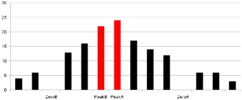
(13) Chapter 2 Literature Review 2.1 Yang-Tsai’s interleaving prediction method Yang and Tsai proposed a reversible data hiding scheme based on interleaving prediction and histogram shifting in 2010 [12]. The interleaving prediction method is used to promote the altitude of the peak point in histogram. It likes a chessboard, as shown in Fig. 2.1, 2.2, and contains two stages. In the first stage, pixels with white-color are processed and predicted by their neighboring pixels of black-color. Then, in the second stage, black-color pixels are processed and predicted by their neighboring white-color pixels. The detailed steps of the first stage are as follows. Let Pi,j be a white-color pixel, where (i, j) is the location, and Di,j be the predicted error between Pi,j and its predictive value. All predicted errors are collected to generate a histogram HS(D). Then, the following steps are executed.. Fig. 2.1 A chessboard with white pixels and black pixels. Pi-1,j Pi,j-1. Pi,j. Pi,j+1. Pi+1,j. Fig. 2.2 A black pixels Pi,j and its neighboring white pixels. 4.

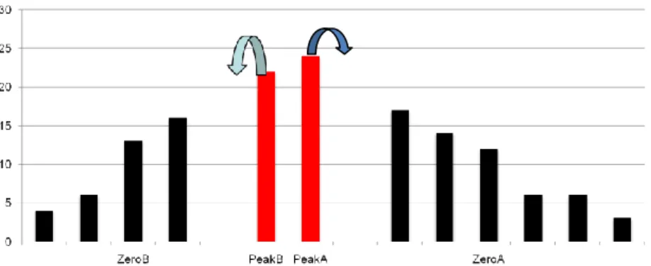
(14) Step 1: Find two pairs of peak and zero points (PeakA, ZeroA) and (PeakB, ZeroB) from the histogram HS(D), such that ZeroB < PeakB < PeakA < ZeroA. Shown as Fig. 2.3:. Fig. 2.3 Two pairs of peak and zero point in the histogram Step 2: Shift the value of the predicted error Di,j by 1 in the following cases. Case A: Change all values in the range of [ ZeroB +1, PeakB-1] to the left by 1 unit. This indicates that D'i,j is set to Di,j-1 as Di,j  [ ZeroB +1, PeakB-1]. Case B: Change all values in the range of [PeakA+1, ZeroA-1] to the right by 1 unit. This shows that D'i,j is set to Di,j +1 as Di,j  [PeakA+1, ZeroA-1]. Shown as Fig. 2.4:. Fig. 2.4 Shift the value of the predicted error in the histogram Step 3: Conceal a secret bit when the predicted error Di,j is equal to PeakA or PeakBc as the following two cases. Case A: If the to-be-embedded bit is 0, predicted error Di,j is unchanged. It indicates that D'i,j is set to Di,j.. 5.

(15) Case B: If the to-be-embedded bit is 1, D'i,j = Di, j  1, if. Di , j  Peak A  D  1 , if D i , j i , j  Peak B . Shown as Fig. 2.5:. Fig. 2.5 If the to-be-embedded bit is 1, PeakA will +1 and PeakB will -1 Step 4: Transform all the predicted errors into pixel values by running the inversed interleaving prediction. Then, output the stego-image. The outputted stego-image is used as the input image of the second stage. The execution of the second stage is similar to that of the first stage. After the second stage is processed, another two pairs of peak and zero points (PeakA, ZeroA) and (PeakB, ZeroB) are created and the final stego-image is obtained.. 2.2 Lee et al.’s prediction-error expansion method The reversible data hiding method proposed by Lee et al. in 2010 is based on difference expansion [13]. This work expanded the DE approach and took the concept of the predicted error and a threshold TH into consideration. For a current pixel Pi,j, they used its left and up adjacent pixels to create a predicted value the predicted error between Pi,j and. Pî , j .. Pî , j. and calculated. To be reversible, the first row and first. column of the image is unused for data hiding and the image is processed from left to right and from top to bottom. The detailed embedding algorithm of Lee et al.’s. 6.

(16) approach is described below. Assume that the left and up adjacent pixels of the current pixel Pi,j are (P1, P2). The predicted value Pî , j is defined as Eq. (1). P  P  Pî , j   1 2   2 . The predicted error is estimated by d.  | Pî , j  Pi , j | . A bit. (1) s is embedded into current. pixel Pi,j according the following cases, where P'i,j is the resulted stego-pixel. Case A: If d  TH , bit s can be hidden by the following function:  Pˆ  2  d  s, if Pî , j  Pi , j P 'i , j   i , j ˆ   Pi , j  2  d  s, o t h e r w i s e. (2). Case B: If d > TH, the current pixel cannot tolerate embedding a secret bit, and this pixel needs to run the following function:  P  (TH  1), if Pî , j  Pi , j P' i , j   i , j  Pi , j  TH , otherwise. (3). 2.3 Li et al.’s general framework method Li et al. proposed a general framework to construct histogram-shifting-based reversible data hiding in 2013 [19]. By the proposed framework, one can get a reversible data hiding algorithm by simply designing the so-called shifting and embedding functions. One of their embedding algorithms is described below. For a 3 × 3 block x = (x1,…, x9) shown in Fig. 2.6, they took the following linear predictor with nonuniform weight to predict x5. x1. x2. x3. x4. x5. x6. x7. x8. x9. Fig. 2.6 A 3x3 block.. 7.

(17) (4) The prediction-error is denoted as e5 =. .. Utilizing smooth pixels for reversible data embedding whereas ignoring the noisy ones will significantly reduce the embedding distortion. Then they took the following function C(x) = max{x1, . . . , x4, x6, . . . , x9}− min{x1, . . . , x4, x6, . . . , x9}. (5). to measure the local complexity of pixel x5 and used an integer-valued parameter s to select smooth pixels. For an integer threshold t > 0, take tl =  t  and tr =  t  . They then defined 2 2 1) S = {x ∈ Z 9 : −tl ≤ e5 < tr ,C(x) < s} and T = Z 9 − S. 2) For x ∈ T ,. 3) For x ∈ S and m ∈ {0, 1}, fm(x) = (x1, . . . , x4, x5 +. +m, x6, . . . , x9).. In the above definitions, S means the set of blocks where each block will be used to embed a secret bit m. T is the set of blocks where each bock will do a shifting operation or nothing.. 8.

(18) Chapter 3 Our proposed methods Our method takes four different prediction methods and their corresponding variance calculations into consideration. Firstly, the cover image is divided into four groups, Group1, Group2, Group3, and Group4, by the interleaving grouping method. Fig. 3.1 shows a grouping result, where each cell indicates a pixel and the number in the cell indicates the group number of the cell. Then, four stages are used to process the four groups, respectively. At each stage, we decide to use the high-capacity tactic or the high-quality tactic first. Then four different prediction methods are evaluated and the one with the largest capacity or the highest efficiency ratio is chosen and used in this stage. Finally, using the chosen prediction method, all of pixels’ predicted errors and variance values are created by their neighboring pixels. Besides, a threshold TH is determined by variance values to decide whether a pixel would join the shifting and embedding process or not. The detail of the data hiding algorithm and extracting and restoring algorithm is given in following subsections.. 1. 2. 1. 2. 1. 3. 4. 3. 4. 3. 1. 2. 1. 2. 1. 3. 4. 3. 4. 3. 1. 2. 1. 2. 1. Fig. 3.1 Interleaving grouping with four groups. 3.1 Data Hiding Algorithm We take the first stage, which processes Group1, to describe our data hiding method.. 9.

(19) As shown in the gray part of Fig 3.1, one Group1 pixel, says Pi,j, is surrounded by eight neighboring pixels which belong to the other groups. Four prediction errors and four variance values of the four prediction methods are calculated as follows. a. Chessboard prediction: For each pixel Pi,j in Group1, its neighboring Group2 and Group3 pixels are chosen to predict Pi,j. The predicted value. i,j. is the averaged. gray value of the chosen pixels. The predicted error Di,j is defined as Pi,j –. i,j.. Besides, a variance value Vi,j is defined as the variance of the chosen pixels. b. Edge prediction: For each pixel Pi,j in Group1, the difference of its neighboring Group2 pixels and the difference of its neighboring Group3 pixels are calculated. The two pixels with the smaller difference value are chosen to predict Pi,j. Then, the predicted error Di,j and the variance value Vi,j are calculated. c. Squared prediction: For each pixel Pi,j in Group1, Pi,j is predicted by the averaged gray value of its neighboring Group2, Group3 and Group4 pixels are chosen to predict Pi,j. Then, the predicted error Di,j and the variance value Vi,j are calculated. d. Max-min-omitted prediction: For each pixel Pi,j in Group1, we use its neighboring Group2 and Group3 pixels excluding the two pixels with the maximal value and the minimal value are chosen to predict Pi,j. Then, the predicted error Di,j and the variance value Vi,j are calculated.. Algorithm Data-Embedding-of-the-First-Stage Input: Cover image I, secret message S, embedding cost C, high-capacity tactic A or high-quality tactic B. Output: Stego image I', the couple data (PeakA, ZeroA) and (PeakB, ZeroB), variance threshold TH, prediction method M. Step 1: For each pixel Pi,j in Group1, a predicted error Di,j is calculated by each of the following four prediction methods M1, M2, M3, and M4: 10.

(20)  M1: Chessboard prediction Case A: If Pi,j is has only two neighboring pixels P1 and P2 belonging to Group2 and Group3, the predicted error Di,j is given as P  P  Di , j  Pi , j   1 2  .  2 . (6). Case B: If Pi,j has only three neighboring pixels P1, P2 and P3 belonging to Group2 and Group3, the predicted error Di,j is given as  P  P  P3  . Di , j  Pi , j   1 2  3 . (7). Case C: If Pi,j is has four neighboring pixels P1, P2, P3 and P4 belonging to Group2 and Group3, the predicted error Di,j is given as  P  P2  P3  P4  . Di , j  Pi , j   1  4 . (8).  M2: Edge prediction Case A: The same to Eq. (6). Case B: The same to Eq. (7). Case C: If Pi,j has two neighboring Group2 pixels P1 and P2 and two neighboring Group3 pixels P3 and P4, the predicted error Di,j is given as  P  P4  If |P1-P2| > |P3-P4|, Di , j  Pi , j   3 ；  2   P  P2  else, Di , j  Pi , j   1 .  2 . (9).  M3: Squared prediction Case A: If Pi,j has only three neighboring pixels P1 , P2 and P3, the predicted error Di,j is given as.  P  P2  P3  Di , j  Pi , j   1 . 3   11. (10).

(21) Case B: If Pi,j has only five neighboring pixels P1, P2, P3, P4 and P5, the predicted error Di,j is given as  P  P  P3  P4  P5  Di , j  Pi , j   1 2 . 5  . (11). Case C: If Pi,j has eight neighboring pixels P1, P2, P3, P4, P5, P6, P7 and P8, the predicted error Di,j is given as P  P  P  P  P  P  P  P  Di , j  Pi , j   1 2 3 4 5 6 7 8  . 8  . (12).  M4: Max-min-omitted prediction Case A: The same to Eq. (6). Case B: The same to Eq. (7). Case C: If Pi,j has four neighboring Group2 and Group3 pixels P1, P2, P3 and P4 with P1≦P2≦P3≦P4, the predicted error Di,j is given as  P  P3  Di , j  Pi , j   2 .  2 . (13). Step 2: For each pixel Pi,j in Group1, a variance value Vi,j is calculated by each of the four prediction methods. The calculations of the four methods are similar, here only the chessboard prediction’s calculation is shown below: Case A: If Pi,j has only two neighboring pixels P1 and P2 belonging to Group2 and Group3, the variance value Vi,j is given as   P  P Vi , j  2   P1   1 2   2 . 2.    P1  P2     P2      2.    . 2.  .  . (14). Case B: If Pi,j has only three neighboring pixels P1, P2 and P3 belonging to Group2 and Group3, the variance value Vi,j is given as 2 2 2    P  P  P   P  P  P   P  P  P   4 Vi, j     P1   1 2 3     P2   1 2 3     P3   1 2 3     3   3 3 3           . .   . (15). Case C: If Pi,j has four neighboring pixels P1, P2, P3 and P4 belonging to Group2 and Group3, the variance value Vi,j is given as. 12.

(22) 2. 2. 2. 2.  P  P  P  P   P  P  P  P   P  P  P  P   P  P  P  P  Vi, j   P1   1 2 3 4     P2   1 2 3 4     P3   1 2 3 4     P4   1 2 3 4   . (16) 4 4 4 4            . Step 3: Case A: If high-capacity tactic A is inputted, for each prediction method Mi, its predicted errors are used to create a histogram. Let the two highest points of the histogram be PeakAi and PeakBi. Then the selected prediction method M is defined as (17) Case B: If high-quality tactic B is inputted, for each prediction method, its efficiency ratio Ri is calculated as follows: Let the numbers of pixels falling in PeakAi, PeakBi, [PeakAi+1, ZeroAi], and [ZeroBi, PeakBi-1] be J1i, J2i, I1i and I2i, respectively. Select the prediction method M with the maximal R value defined as (18) Step 4: The selected method M is used to process Group1 to embed secret data. Using method M, let its predicted errors Di,j, variance values Vi,j, two pairs of peak and. zero. points. (PeakA,. ZeroA). and. (PeakB,. ZeroB). with. ZeroB<PeakB<PeakA<ZeroA have been calculated. Two arrays Vpeak, and Vshift are created, where their rth elements are defined as Vpeak[r] = |{Pi,j | Pi,j ∈ Group1, Di,j = PeakA or PeakB, Vi,j= r}|. (19). Vshift[r] = |{Pi,j| Pi,j ∈ Group1, Di,j ∈ [PeakA+1, ZeroA], or [ZeroB, PeakB-1],. Vi,j = r}|. (20). where r is a non-negative integer and |.| means the size of the set. Step 5: Using the embedding cost C, TH is the maximal non-negative value satisfying. (21) 13.

(23) Step 6: Use TH to distinguish whether a Group1’s pixel Pi,j will join the shifting and embedding process or not by setting the following flag: 1 , if Vi,j  TH . Flag i , j   0 , if Vi,j  TH .. If Flagi,j = 0, it means that the pixel Pi,j in Group1 will not join the shifting and embedding process; If Flagi,j = 1, it means that the pixel Pi,j in Group1 will join the shifting and embedding process. Step 7: Run the following cases for each predicted error Di,j and its variance Vi,j. Case A: If Flagi,j = 1 and the predicted error Di,j is equal to PeakA or PeakB, fetch a secret bit from S and do the following two cases: Case A1: If to-be-embedded-bit is 0, D'i,j is set to Di,j. Case A2: If to-be-embedded-bit is 1,  If Di , j  Peak A , D'i , j  Di , j  1   If Di , j  Peak B , D'i , j  Di , j  1.. Case B: If Flagi,j = 1 and the predicted error Di,j falls into the range of [ZeroB +1, PeakB－1] or [PeakA +1, ZeroA－1], shift predicted error Di,j by one unit as follows:  If Di , j  [ Peak A  1, ZeroA  1], D'i , j  Di , j  1   If Di , j  [ ZeroB  1, Peak B  1], D'i , j  Di , j  1.. Case C: If Flagi,j = 0, do nothing, that is, D'i,j is set to Di,j. Step 8: Transform each predicted error D'i,j into pixel value P'i,j by the inverse of the prediction method M. Finally, all pixel values P'i,j form the stego-image I'. Step 9: Output two pairs (PeakA, ZeroA) and (PeakB, ZeroB), a variance threshold TH, and a prediction method M. The above algorithm, which processes Group1, is for the first stage of level-one data hiding. For saving the run time, the second, third, and fourth stages will use the same selected method M of the first stage. In Step 5, if none of r values satisfies Eq. (21), TH will not exist. In this case, none of secret data will be embedded in this stage. 14.

(24) To avoid that none of data can be embedded in the next following levels, we increase the embedding cost C by a fixed value whenever a new level is processed. Note that the outputted parameters in Step 9 can be seen as secret data and can be embedded in the next stage. So, only the outputted parameters of the last stage cannot be embedded.. 3.2 Data Extracting and Recovering Algorithm The data extracting and recovering algorithm is similar to the data embedding algorithm. Following shows the detailed steps of the data extracting and recovering algorithm for the last stage.. Algorithm Extracting-and-Recovering-of-the-Last-Stage Input: Stego image I', two pairs (PeakA, ZeroA) and (PeakB, ZeroB), a variance threshold TH, a prediction method M, high-capacity tactic A or high-quality tactic B. Output: Cover image I, secret message S. Step 1: For each pixel P'i,j of stego-image I', compute its predicted error D'i,j and variance value V'i,j by the prediction method M. Step 2: For each predicted error D'i,j and its variance value V'i,j, run the following data extracting and pixel recovering process. If V'i,j > TH, do nothing, that is, Di,j = D'i,j. If V'i,j  TH, do the following cases. Case A: If the predicted error D'i,j is equal to PeakA or PeakB, obtain a secret bit 0 and recover the predicted error as Di,j = D'i,j. Case B: If D'i,j = PeakA+1, extract a secret bit 1 and recover the predicted error as Di,j = D'i,j－1. 15.

(25) If D'i,j = PeakB－1, extract a secret bit 1 and recover the predicted error as Di,j = D'i,j+1. Case C: If D'i,j falls into the range of [ZeroB, PeakB－2], recover the predicted error as Di,j = D'i,j+1. If D'i,j falls into the range of [PeakA+2, ZeroA], recover the predicted error as Di,j = D'i,j－1. Step 3: Transform all predicted errors Di,j into pixels Pi,j to form the cover image I. Step 4: Output the cover image I and all extracted message S. Note that variance value V'i,j in the data extracting and recovering process is the same to the variance value Vi,j in the corresponding data hiding process. The reason is that both Vi,j and V'i,j are calculated from neighboring pixels, which are unchanged when a after the corresponding data hiding process is finished. Therefore, V'i,j can be used to judge whether D'i,j joins the data extracting and pixel recovering process.. 3.3 Overflow/Underflow Overflow and underflow happens when the shifting and embedding process causes a pixel’s value over value 255 or under value 0. To cope with this issue, we pre-modify the pixels which may occur overflow or underflow and use a location map to record this information. This information can be seen as a part of secret data and be embedded into the cover image. In our Histogram-based reversible data hiding method, each pixel will change ±1 at most in every level. Therefore, before embedding secret data into the image in one level, we pre-modify pixels with values 0 and 255 into pixels with values 1 and 254, respectively, to prevent overflow and underflow as follows:  1, if Pi , j  0 Pi , j   254, if Pi , j  255.. 16.

(26) Also, to judge those modifications, the location map is created before those modifications as follows: 0, if Pi , j  1 or Pi , j  254 L[k ]    1, if Pi , j  0 or Pi , j  255,. where k is an index for those recorded pixels. Therefore, in each level, the size of the location map is k bits if there are k pixels with values equal to values 0, 1, 254, or 255.. 17.

(27) Chapter 4 Experimental results In this section, we provide the resultant of embedding capacity and image quality to demonstrate the performance of our proposed scheme. In our experiment, ten gray images with size 512×512, which are depicted in Fig. 4.1 and Fig. 4.2, are used, and the secret message is obtained by random generation. To estimate the image quality, we applied the function of peak-signal-to-noise-ratio (PSNR), which is defined as Eq. (21). To estimate the embedding capacity, the function of ER (Embedded Ratio; bpp) is adopted, where ER = Total Embedded bits / Size of Cover image. In the experiment, the embedding cost C is set to 30 at the first level. Then, the C value is added by 0.5 at each of the following levels. PSNR  10  log10 (. 2552 ), MSE. (21). where MSE is the mean square error between the cover image and the stego-image.. (a). (b). (d). (c). (e). Fig. 4.1 The cover images with size 512×512; (a) Airplane; (b) Baboon; (c) Boat; (d) Lena; (e) Peppers. 18.

(28) (a). (b). (d). (c). (e). Fig. 4.2 The cover images with size 512×512; (a) Barb; (b) Girl; (c) Gold; (d) Toys; (e) Zelda. Table 4.1. Each image’s capacity, PSNR, and the prediction M at every level. (high-capacity tactic A, embedding cost C = 30) Image Level 1. Level 4. Level 7. Level 10. Level 20. Airplane. Baboon. Boat. Lena. Peppers. Capacity. 103956. 31719. 58759. 99936. 85550. PSNR. 51.17. 55.10. 51.01. 49.06. 48.91. M. M1. M4. M2. M1. M1. Capacity. 272609. 130702. 192922. 255913. 223195. PSNR. 43.12. 43.69. 41.60. 40.92. 39.82. M. M3. M2. M2. M2. M4. Capacity. 394342. 207013. 277664. 363636. 306574. PSNR. 39.15. 39.47. 38.23. 36.18. 37.38. M. M1. M2. M2. M2. M1. Capacity. 479299. 270876. 353120. 432191. 388137. PSNR. 35.84. 37.38. 35.63. 34.48. 35.44. M. M1. M2. M2. M4. M4. Capacity. 687704. 470440. 510963. 629919. 570497. PSNR. 31.65. 32.46. 30.02. 29.49. 30.31. M. M4. M4. M2. M2. M2. 19.

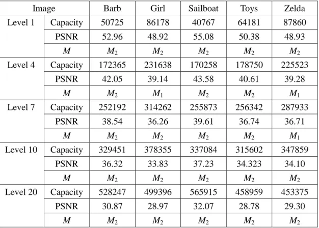
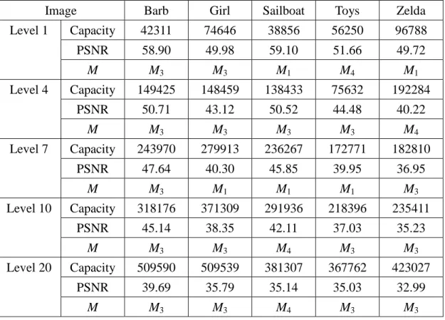
(29) Table 4.2. Each image’s capacity, PSNR, and the prediction M at every level. (high-capacity tactic A, embedding cost C = 30) Image Level 1. Level 4. Level 7. Level 10. Level 20. Barb. Girl. Sailboat. Toys. Zelda. Capacity. 50725. 86178. 40767. 64181. 87860. PSNR. 52.96. 48.92. 55.08. 50.38. 48.93. M. M2. M2. M2. M2. M2. Capacity. 172365. 231638. 170258. 178750. 225523. PSNR. 42.05. 39.14. 43.58. 40.61. 39.28. M. M2. M1. M2. M2. M1. Capacity. 252192. 314262. 255873. 256342. 287933. PSNR. 38.54. 36.26. 39.61. 36.74. 36.71. M. M2. M2. M2. M2. M1. Capacity. 329451. 378355. 337084. 315602. 347859. PSNR. 36.32. 33.83. 37.23. 34.323. 34.10. M. M2. M2. M2. M2. M2. Capacity. 528247. 499396. 565915. 458959. 453375. PSNR. 30.87. 28.97. 32.07. 28.78. 29.30. M. M2. M2. M2. M2. M2. Table 4.3. Each image’s capacity, PSNR, and the prediction M at every level. (high-quality tactic B, embedding cost C = 30) Image Level 1. Level 4. Level 7. Level 10. Level 20. Airplane. Baboon. Boat. Lena. Peppers. Capacity. 103956. 16873. 60215. 90345. 79711. PSNR. 51.17. 61.70. 47.56. 49.39. 49.65. M. M1. M3. M1. M4. M4. Capacity. 282135. 61429. 207521. 239069. 209481. PSNR. 43.30. 53.90. 39.95. 41.37. 40.23. M. M4. M3. M3. M3. M2. Capacity. 398864. 112359. 338425. 331799. 299571. PSNR. 40.12. 48.48. 37.23. 39.88. 38.73. M. M4. M1. M3. M3. M3. Capacity. 507270. 144627. 466401. 416004. 362713. PSNR. 37.64. 47.72. 34.51. 38.00. 37.27. M. M2. M3. M1. M3. M3. Capacity. 731523. 264966. 654985. 623648. 533181. PSNR. 33.05. 44.20. 32.23. 34.58. 32.81. M. M1. M3. M4. M3. M3. 20.

(30) Table 4.4. Each image’s capacity, PSNR, and the prediction M at every level. (high-quality tactic B, embedding cost C = 30) Image Level 1. Level 4. Level 7. Level 10. Level 20. Barb. Girl. Sailboat. Toys. Zelda. Capacity. 42311. 74646. 38856. 56250. 96788. PSNR. 58.90. 49.98. 59.10. 51.66. 49.72. M. M3. M3. M1. M4. M1. Capacity. 149425. 148459. 138433. 75632. 192284. PSNR. 50.71. 43.12. 50.52. 44.48. 40.22. M. M3. M3. M3. M3. M4. Capacity. 243970. 279913. 236267. 172771. 182810. PSNR. 47.64. 40.30. 45.85. 39.95. 36.95. M. M3. M1. M1. M1. M3. Capacity. 318176. 371309. 291936. 218396. 235411. PSNR. 45.14. 38.35. 42.11. 37.03. 35.23. M. M3. M3. M4. M3. M3. Capacity. 509590. 509539. 381307. 367762. 423027. PSNR. 39.69. 35.79. 35.14. 35.03. 32.99. M. M3. M3. M4. M3. M3. Tables 4.1, 4.2, 4.3 and 4.4 show that our approach will choose the best prediction method M at every level. Therefore we can embed more secret data more efficiently at every. Moreover, because the predictions have different characteristics, it can avoid using the same prediction at every level and some regions of pixels change may too large. Table 4.5. The compared result among our approach (embedding cost C = 30), Lin’s, Hsiao’s and Yang’s schemes. Images Lin et al.’s. Hsiao et. method [10] al.’s method [22]. Lin and. Yang and. Our. Our. Hsueh’s. Tsai’s. approach. approach. method [21] method [12] (capacity). (R). Airplane. 362847. 286488. 367392. 397712. 742082. 750408. Baboon. 230079. 138398. 162544. 184468. 576014. 575917. 21.

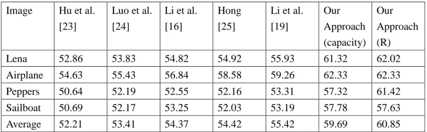
(31) Boat. 314196. 266724. 307937. 294944. 510963. 513744. Lena. 346568. 303700. 309166. 420986. 596903. 604839. Peppers. 342175. 303736. 356450. 374837. 570497. 557048. Average. 319173. 259809. 300698. 334589. 599291. 600391. Ratio. 53.16%. 43.27%. 50.08%. 55.72%. 99.81%. 100%. PSNR. 30.19. 30.00. 30.26. 30.25. 30.27. 32.75. From the compared result in Table 4.5, we can find out that our approach clearly have more capacity when the PSNR values are similar. We promote at least 44% capacity than that of other methods. The reason is that our approach uses the more suitable prediction method at every level. We also have some overhead. For each level we need 80 bits to record four peak points and zero points, 32 bits for TH, and 2 bits for the prediction M. If we hide 20 levels, we need 2280 bits to record the overhead. Table 4.6 shows the comparison among Hu et al.’s method [23], Luo et al.’s method [24], Li et al.’s method [16], Hong’s method [25], Li et al.’s method [19], and our proposed scheme. From this table, our scheme has better image quality than that of other methods when the size of the embedded bits is 20000. The reason is that our approach forbids some prediction errors entering the process of pixel shifting and we use four different prediction methods. The threshold TH strategy in our proposed scheme has efficiently eliminated the distortion caused by pixel shifting. It therefore has good performance of PSNR than that of the previous works. Fig. 4.3 shows the PSNR values between our approach using tactic A and Yang-Tsai method [12] based on various embedded capacities. From Fig. 4.3, the average PSNR value of Yang-Tsai method is 52.52 dB, and our approach is about 61.18 dB, which is significantly improved by 8.66 dB.. 22.

(32) Fig. 4.3 The PSNR comparison of Lena image between our approach and Yang and Tsai’s scheme based on various hiding payload.. Table 4.6. The compared result between our approach and other schemes, for an embedding capacity of 20000 bits. Image. Hu et al. [23]. Luo et al. [24]. Li et al. [16]. Hong [25]. Li et al. [19]. Our Approach (capacity). Our Approach (R). Lena. 52.86. 53.83. 54.82. 54.92. 55.93. 61.32. 62.02. Airplane. 54.63. 55.43. 56.84. 58.58. 59.26. 62.33. 62.33. Peppers. 50.64. 52.19. 52.55. 52.16. 53.31. 57.32. 61.42. Sailboat. 50.69. 52.17. 53.25. 52.03. 53.19. 57.78. 57.63. Average. 52.21. 53.41. 54.37. 54.42. 55.42. 59.69. 60.85. In addition, we also compared the result with the previous work of Lee et al.’s scheme, as shown in Table 4.7. From this table, it is obvious that the averaged stego-image qualities of Lean and Baboon in our scheme are larger than that of Lee et al.’s scheme. As shown in Fig. 4.4, our scheme with tactic A has better image quality than previous works [10, 12, 15, 20] with the same embedding capacities.. 23.

(33) Table 4.7. Comparison between Lee et al.’s scheme and our proposed scheme with the same embedding ratio.. Lena Baboon. Lee et al.’s scheme [13]. Our approach (capacity). Our approach (R). ER(bpp). PSNR. ER(bpp). PSNR. ER(bpp). PSNR. 0.14. 48.47. 0.14. 58.59. 0.14. 58.89. 0.98. 32.17. 0.98. 46.92. 0.98. 46.30. 0.05. 48.25. 0.05. 62.92. 0.05. 63.11. 0.62. 30.02. 0.62. 46.48. 0.62. 47.39. (a). (b). Fig. 4.4 Comparison results among our proposed scheme and other reversible schemes for images: (a) Lena; (b) Baboon. As shown in Fig.4.5 and Fig. 4.6, the original images and the stego-images are shown for comparison when the capacities are approaching to 300000 bits using tactic A. It is visually difficult to distinguish between the original image and the stego-image for both Lena and Baboon by human eyes.. 24.

(34) (a). (b). Fig.4.5 (a) Original image Lena. (b) Stego-image Lena with capacity =300288 bits and PSNR =39.054 dB.. (a). (b). Fig.4.6 (a) Original image Baboon. (b) Stego-image Baboon with capacity =317015 bits and PSNR =36.304 dB. Table 4.8 shows the occurrence times of overflow for each image after 20-level data hiding. Compared to the capacity of each image, these overflow data can be easily hidden into the stego-image.. Table 4.8. Each image’s overflow after 20-level data hiding. Images. Airplane. Baboon. Boat. Lena. Peppers. Overflow. 0. 21. 8. 0. 1644. Images. Barb. Girl. Sailboat. Toys. Zelda. Overflow. 251. 539. 0. 2214. 0. 25.

(35) Chapter 5 Conclusions In this study, we propose a reversible data hiding method based on four candidates of prediction methods and local complexity for enhancing stego-image quality. We evaluate the four prediction methods by two ways to decide which prediction method will be used. First, if we want to achieve high-capacity, we evaluate prediction methods’ capacities. Second, if we want to achieve high-quality, we evaluate the prediction methods’ efficiency ratios. Also we use the variance strategy to find out a threshold TH for selecting which pixel should join the process of pixel shifting and data concealing. The variance strategy has efficiently improved histogram-based approaches to obtain high image quality. From the experimental result, it shows that our method owns higher image capacity and quality than that of previous works.. 26.

(36) References. [1] J. B. Feng, I. C. Lin, C. S. Tsai, and Y. P. Chu, “Reversible watermarking: Current status and key issues,” International Journal of Networks and Security, vol. 2, no. 3, pp. 161-170, 2006. [2] Y. Q. Shi, Z. Ni, D. Zou, C. Liang, and G. Xuan, “Lossless data hiding: Fundamentals, algorithms, and applications,” in Proc. IEEE ISCAS, 2004, pp. 33-36. [3] D. C. Lou, M. C. Hu, and C. Li Liu, “Multiple-layer data hiding scheme for medical image,” Computer Standards and Interfaces, vol. 31, no. 2, pp. 329-335, 2010. [4] Q. M. Al-Qershi and B. E. Khoo, “High capacity data hiding schemes for medical images based on difference expansion, ”Journal of Systems and Software, vol. 31, no. 4, pp. 787-794, 2011. [5] J. Tian, “Reversible data embedding using a difference expansion,” IEEE Trans. on Circuits Systems for Video Technology, vol. 16, no. 3, pp. 890-896, 2003. [6] A. M. Alttar, “Reversible watermark using the difference expansion of a generalized integer transform,” IEEE Trans. on Image Processing, vol. 13, no. 8, pp. 1147-1156, 2004. [7] C. C. Lee, H. C. Wu, C. S. Tsai, and Y. P. Chu, “Adaptive lossless steganography with centralized difference expansion,” Pattern Recognition, vol. 141, no. 6, pp. 2097-2106, 2008. [8]. Z. Ni, Y. Q. Shi, N. Ansar, and W. Su, “Reversible data hiding,” IEEE Trans. on Circuits Systems for Video Technology, vol. 16, no. 3, pp. 354-362, 2006.. [9] S. Yousefl, H. Rablee, E. Yousefl, and M. Ghanbarl, “Reversible data hiding 27.

(37) using histogram sorting and integer transform,” in Proc. IEEE DEST, 2007, pp. 487-490. [10] C. C. Lin, W. L. Tai, C. C. Chang, “Multilevel reversible data hiding based on histogram modification of difference images,” Pattern Recognition, vol. 41, no. 12, pp. 3582-3591, 2008. [11] P. Tsai, Y. C. Hu, and H. L. Yeh, “Reversible image hiding scheme using predictive coding,” Signal Processing, vol. 89, no. 6, pp. 1129-1143, 2009. [12] C. H. Yang and M. H. Tsai, “Improving histogram-based reversible data hiding by interleaving prediction,” IET Image Processing, vol. 4, no. 4, pp. 223-234, 2010. [13] C. F. Lee, H. L. Chen, and H. K. Tso, “Embedding capacity raising in reversible data hiding based on prediction of difference expansion,” Journal of Systems and Software, vol. 83, no. 10, pp. 1864-1872, 2010. [14] A. Zhao, H. Luo, Z. M. Lu, J. S. Pan, “Reversible data hiding based on multilevel histogram modification and sequential recovery,” AEU-International Journal of Electronics and Communication, vol. 65, no. 10, pp. 814-826, 2011. [15] H. J. Hwang, H. J . Kim, V. Sachnev, and S. H. Joo, “Reversible watermarking method using optimal histogram pair shifting based on prediction and sorting,” KSII Trans. on Internet and Information Systems, vol. 4, no. 4, pp. 555-670, 2010. [16] X. Li, B. Yang, and T. Zeng, “Efficient reversible watermarking based on adaptive prediction-error expansion and pixel selection,” IEEE Trans. on Image Processing, vol. 20, no. 12, pp. 3524-3533, 2011. [17] W. L. Tai, C. M. Yeh, and C. C. Chang, “Reversible data hiding based on histogram modification of pixel differences,” IEEE Trans. on Circuits Systems for Video Technology, vol. 19, no. 6, pp. 906-910, 2009. 28.

(38) [18] Z. Zhao, H. Luo, Z.M. Lu, J.S. Pan, “Reversible data hiding base on multilevel histogram modification and sequential recovery” International Journal of Electronics and Communications (AEU), Int. J. Electron. Commun. (AEU) 65 814–826, 2011. [19] X.. Li,. B.. Li,. B.. Yang,. and. T.. Zeng,. “General. framework. to. histogram-shifting-based reversible data hiding” IEEE Transactions on image processing, vol. 22, no. 6, June 2013. [20] C. Y. Weng, C. H. Yang, C. I. Fan, K. L. Liu, and H. M. Sun, “Histogram-Based Reversible Information Hiding Improved by Prediction with the Variance to Enhance Image Quality,” in The 8th Asia Joint Conference on Information Security, Seoul, Korea, July 25-26, 2013. [21] C.C. Lin and N.L. Hsueh, “A lossless data hiding scheme based on three-pixel block differences,” Pattern Recognition, 2008, Vol. 41, No. 4, pp. 1415-1425. [22] J.Y. Hsiao, K.F. Chan, and J.M. Chang, “Block-based reversible data embedding,” Signal Processing, 2009, Vol. 89, Issue 4, pp. 556-569. [23] Y. Hu, H. K. Lee, and J. Li, “DE-based reversible data hiding with improved overflow location map,” IEEE Trans. Circuits Syst. Video Technol., vol. 19, no. 2, pp. 250–260, Feb. 2009. [24] L. Luo, Z. Chen, M. Chen, X. Zeng, and Z. Xiong, “Reversible image watermarking using interpolation technique,” IEEE Trans. Inf. Forens. Security, vol. 5, no. 1, pp. 187–193, Mar. 2010. [25] W. Hong, “Adaptive reversible data hiding method based on error energy control and histogram shifting,” Opt. Commun., vol. 285, no. 2, pp. 101–108, 2012.. 29.

(39)