以Laguerre模型為基礎之線性與非線性程序的鑑別與控制

行政院國家科學委員會專題研究計畫 成果報告

以 Laguerre 模型為基礎之線性與非線性程序的鑑別與控制 研究成果報告(精簡版)

計 畫 類 別 ： 個別型

計 畫 編 號 ： NSC 98-2221-E-006-062-

執 行 期 間 ： 98 年 08 月 01 日至 99 年 07 月 31 日 執 行 單 位 ： 國立成功大學化學工程學系（所）

計 畫 主 持 人 ： 黃世宏

計畫參與人員： 碩士班研究生-兼任助理人員：謝楚御 碩士班研究生-兼任助理人員：李長青 碩士班研究生-兼任助理人員：王銘賢 碩士班研究生-兼任助理人員：許書維 博士班研究生-兼任助理人員：柳水金

報 告 附 件 ： 出席國際會議研究心得報告及發表論文

處 理 方 式 ： 本計畫可公開查詢

中 華 民 國 99 年 10 月 25 日

以 Laguerre 模型為基礎之線性與非線性程序的鑑別與控制

計畫編號：NSC 98-2221-E-006-062

主持人：黃世宏 成功大學化工系教授

摘要

無法預測之擾動會造成鑑別線性離散多重輸 入/多重輸出模型的實際困難。本計畫使用含 可調時間縮放因子的 Laguerre 模型來建立回 歸方程式，其部分組成項為初使狀態以及在 未知時間進入鑑別測試的負載擾動。所產生 之 Laguerre 係數最小平方估測可用來有效和 正確地建構程序與擾動模型。擴增階次的概 念被引入來處理負載擾動動態與程序動態相 異的情況。針對決定性負載擾動，可透過兩 個誤差標準的最小化來選擇適當的時間縮放 因子、擾動進入時間與程序時延，以確保程 序模型的正確性；針對隨機性擾動，可透過 另一個誤差標準的最小化來選擇適當的時間 縮放因子與程序時延，以去除擾動所造成的 負面效應。

本計畫亦 發展一 非疊代方法來鑑別非線性 Wiener 模型，其關鍵為使用 Laguerre 展開式 來描述線性動態，並使用含參考點之逆多項 式函數來近似靜態非線性。如此 Laguerre 與 多項式係數之最小平方估測可以非疊代方式 獲得。為增加線性與非線性部分的估測正確 性，誤差標準被建立來選擇適當的時間縮放 因子和輸出參考值，它們分別與 Laguerre 展 開式和多項式近似的有效性有關。所鑑別之 Wiener 模型可輕易用來設計非線性控制器。

關鍵詞：系統鑑別、Laguerre模型、確定性擾 動、隨機性擾動、Wiener程序、非線性控制 設計、非疊代演算法

Abstract

Unpredicted disturbances impose practical difficulties on the identification of linear discrete multiple-input/multiple-output models from plant tests. This project establishes an identification method based on Laguerre models

with adjustable time-scaling factors. A linear regression equation is derived to incorporate the terms concerning initial states as well as disturbances occurring before and after the start of the identification test. The resulting least- squares estimator of the Laguerre coefficients is thus employed to develop process and disturbance models efficiently and accurately.

The idea of augmented order is introduced to account for distinct load dynamics. To improve identification under deterministic disturbances, two error criteria are developed to infer the proper values of the time-scaling factor, the load entering time, and process time delays. In the presence of a stochastic disturbance, another error criterion is presented to determine the time- scaling factor that rejects the most deteriorating effect of the stochastic disturbance on parameter estimation.

This project also develops a noniterative method to identify a nonlinear Wiener model. The key idea is to describe the linear dynamics by a Laguerre expansion and approximate the static nonlinearity by an inverse polynomial function with a reference point. The resulting least- squares estimator of the Laguerre and polynomial coefficients is thus obtainable in a noniterative manner. To improve the estimation accuracy of both linear and nonlinear parts, error criteria are established to infer proper values of the time-scaling factor and output reference value, which are crucial to the effectiveness of the Laguerre expansion and the polynomial function, respectively. The identified Wiener model can be easily employed to design a nonlinear controller.

Keywords: System Identification, Laguerre Model, Deterministic Disturbance, Stochastic Disturbance, Wiener Process, Nonlinear Control Design, Noniterative Algorithm

1. Introduction

Unsteady initial states and ubiquitous disturbances of unpredicted nature impose practical difficulties on the identification of linear parametric models from plant tests.

Identification under unknown disturbances has not been fully resolved because of the lack of a proper investigation into the practical problems delineated below. First, the unknown disturbance dynamics could be widely different from the process dynamics. Second, the load disturbance is likely to occur at an unknown time during a plant test. Third, the disturbance affecting the identification test can be either deterministic or stochastic.

Many of the available identification methods are restricted to predetermined test conditions and a specific type of disturbance. Hang et al.

(1993), Shen et al. (1996), and Park et al. (1997) proposed corrective or iterative procedures to remove the biasing effect caused by a static load disturbance on a relay test. Wang et al. (2006) developed an identification method based on a multiple integration approach and relay tests under nonzero initial conditions and static load disturbances. These methods may not be valid for non-static load disturbances occurring during the test.

As a remedy, Hwang and Wang (2003) developed a time- and frequency-weighted integral approach for identification from relay tests under non-static load disturbances. The properly chosen frequency weighting could reject the low-frequency content of distinct load dynamics. Liu and Gao (2008) presented an identification method based on step-like tests. In this method, a polynomial function in time is employed to fit the transient behavior of the load disturbance and a multiple integration is exploited to derive a linear regression equation for parameter estimation. However, these methods can cope only with a partial class of deterministic and stochastic disturbances.

The aforementioned identification methods were proposed to find continuous-time models or frequency-response data for single- input/single-output (SISO) systems. The corresponding algorithms cannot obtain good discrete-time models provided the sample time is

varied widely as required by the data acquisition system. On the other hand, Wahlberg (1991) has shown that identification using discrete Laguerre models is insensitive to the choice of the sample time and possesses good asymptotic statistical properties for least-squares estimation.

A partial objective of this project is to develop a method that identifies discrete parametric models using test data distorted by unknown initial states and disturbances for linear multiple- input/multiple-output (MIMO) systems. A Laguerre ARX (autoregressive with exogenous input) model structure of augmented order in conjunction with an adjustable time-scaling factor is generalized to derive a linear regression equation that incorporates the terms concerning initial states and disturbances entering any time during the identification test. The least-squares estimator of the Laguerre coefficients could result in accurate process and disturbance models.

2. Discrete Laguerre Expansion

Assume that the discrete transfer function G(z) is strictly proper (G(∞)＝0), analytic in z 1, and continuous in

z

1. For

1, there exists

a sequence { }

g

_i such that

1

( )

_{i i}

( , )

i

G z

^

g L z 



 

^(1a)

and

2 1

(1 ) 1 ( , )

i i

T z

L z z z

 

  

  

     (1b)

where

 is a time-scaling factor, g

_i is the Laguerre coefficients, and T is the sample time.

Equations (1a) and (1b) constitute the discrete Laguerre Expansion (Wahlberg, 1991). The orthogonal functions given in Eq. (1b) are the Laguerre functions with single poles in

. It has

been revealed that with a good choice of

, Eq.

(1a) can be approximated well by the partial sum of r terms:

1

( ) ( , )

r i i i

G z g L z 



 

⁽²⁾

We denote Eq. (2) as a Laguerre FIR (finite impulse response) model. For a fast rate of

convergence, T/(1–

) should be set close to the

dominating time constants of the system (Wahlberg, 1991).

An alternative is to represent G(z) by a Laguerre ARX model as follows:

1

1

( , ) ( )

1 ( , )

n i i i

n i i i

b L z G z

a L z













 





⁽³⁾

where

a and

_i

b denote

_i the Laguerre coefficients. In general, G(z) can also be expressed by

( ) ( )

( )

G z B z



A z

(4)

where A(z) and B(z) are the denominator and numerator polynomials, respectively.

1

( )

n

n n i

i i

A z z a z

^



  

^(5a)

1

( )

n n i i i

B z b z

^



 

^(5b)

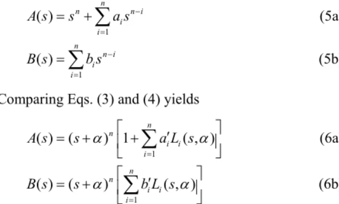
Comparing Eqs. (3) and (4) yields

1

( ) ( ) 1 ( , )

n n

i i i

A z z  a L z 



  

  



 ^(6a)

1

( ) ( ) ( , )

n n

i i i

B z z  b L z 



  

  



 ^(6b)

This gives rise to the conversion relationships between the coefficients a

i

, b

i

and

a,

_i

bfor

_i

1, 2, ,

i   n

. Unlike the Laguerre FIR model, the Laguerre ARX model is no longer an approximation and the selection of

does not

affect the accuracy of model parameter estimation. Nevertheless, the setting of

 is

crucial for identification under deterministic and/or stochastic disturbances as will be elaborated later.

3. Identification via Laguerre Models under Deterministic and Stochastic Disturbances 3.1 SISO process identification

We first consider a SISO system subject to unsteady initial conditions, deterministic load disturbances, and stochastic disturbances as

described by the following z-transform equation:

L

P D I L1

L2 V

( ) ( ) ( ) ( ) ( ) ( ) ( ) ( ) ( ) ( )

Y z G z U z G z G z S z

G z S z z

^

G z E z

  

  (7)

where Y(z) and

U

_D( )

z are the z-transforms ( Z [ ] 

) of the output variable y(k) measured at discrete time instants t = kT (

k  0,1, 2 

) and the delayed input excitation

u

_D( )

k (= u(k



)) with

being an integer delay, respectively. Note that k

= 0 corresponds to the initial time t

_i

of observed output data collected for computation algorithms, and the applied input variable u(k) could be of any value for k < 0. The z-transforms

G z and

_P( )

I( )

G z denote a strictly proper process transfer

function of order n

P

and unsteady initial conditions, respectively. The stochastic disturbance is represented by a zero-mean white noise signal E(z) (

 Z e k [ ( )]

) and a pulse transfer function

G

_V( ).

z

It should be noted that the problem of bounded deterministic disturbances is dealt with in a rather deliberate manner. Despite the fact that load disturbances may enter the system at any unknown instants, we simulate all of their effects by two sequential equivalents. The first load disturbance, occurring at k = 0, is obtained by passing a unit step change

S z ( )

(= z

/

(z1)) through a load transfer function

G

_L1( ),

z

whereas the second load disturbance, presumed to enter at a later unknown time k =

 L

, is given by passing a delayed unit step change

S z z

( ) ^L through a load transfer function

G

_L2( ).

z

If all load disturbances are known to occur before the initial time t

_i

, then the second load disturbance can be removed to simplify Eq. (7).

Ignoring the stochastic disturbance term momentarily and replacing each transfer function by its appropriate denominator and numerator polynomials, Eq. (7) reduces to

L

P I

P P

1

L1 L2

P L1 P L2

( ) ( )

( ) ( )

( ) ( )

( ) ( )

( 1) ( ) ( ) ( 1) ( ) ( )

D

B z zB z

Y z U z

A z A z

zB z z B z

z A z A z z A z A z



 

 

 

 

(8)

where

B z

_P( ),

B z

_I( ),

B

_L1( ),

z

and

B

_L2( )

z

are

polynomials of degrees

n

_P1,

n

_P1,

n

_P

n

_L1, and

n

_P

n

_L2, respectively, and

A z

_P( ),

A

_L1( ),

z

and

A

_L2( )

z are monic polynomials of degrees n ,

_P

n , and

L1

n , respectively.

_L2

Equation (8) reveals that each load disturbance is composed from dynamics similar to and those distinct from the process dynamics

A z

_P( ).

Without loss of generality, we assume that

L1( )

B z and B

_L2( )

z are coprime with A

_L1( )

z and

L2( ),

A z

respectively, and

A z is coprime with

_P( )

P( ),

B z A

_L1( ),

z A

_L2( ).

z

As a result,

A

_L1( )

z

and

L2( )

A z

denote the distinct dynamics of load disturbances and their least common multiple forms a monic polynomial

A z of degree n

_L( )

L

. Using partial fraction expansions and letting

P L

( ) ( ) ( )

A z



A z A z

and

B z

( ) 

B

_P( )

z A

_L( ),

z

we can rearrange Eq. (8) as follows:

L L

0 D

1 1

0

( )

( ) ( )

( ) ( )

( ) ( ) ( 1) ( )

( )

( )

( ) ( 1) ( )

n

n

c z z

B z zC z

Y z U z

A z A z z A z

d z z z D z

A z z A z









 

 

   



 

 



(9)

where

A z ( )

and

B z ( ),

as defined in Eqs. (5a) and (5b), represent the process of augmented order

n

  . Substituting Eqs. (6a) and (6b)

n

_P

n

_L in Eq. (9) and multiplying both sides of the resulting equation by

1

1 ( , )

n i i i

a L z 



  

leads to the underlying equation for parameter estimation in terms of the Laguerre ARX model:

L L

D

1 1

0

1

1

1 0

1

( ) ( , ) ( ) ( , ) ( )

( , ) 1 ( , )

1

n n

i i i i

i i

n

i i

i n

i i

i

Y z a L z Y z b L z U z

c zL z c z z d z L z d z

z

 

 





 



   



 

 

 

 



 

 



 





(10)

Note that the last two terms on the right-hand side of the above equation can be used to construct the second load disturbance, if any, as follows:

  

L2 0

1

( )

( ) ( 1) ,

n n

i i i

G z z d z d L z

A z

 



    

       

⁽¹¹⁾

Taking the inverse z-transform on Eq. (10) gives

rise to the regression equation for

0,1, , 1

k   N 

:

 D,

1 1 1

0 L 0 L

1

( ) ( ) ( )

( ) ( )

n n n

i i i i i i

i i i

n

i i i

y k a y k b u k c k

c d k  d I k 

  



  

  

  

    

  



   

 

(12)

where

y k

i^,

u

D,_i

k

, and i

k

are the inverse z-transforms of

L z

_i

( , ) ( ),  Y z L z

_i

( , )  U

_D

( ), z

and

zL z

_i

( , ), 

respectively; further,

L L

( ) 0 if

i

k







k







L L

L

( ) 1 if

0 if

I k k

k

 



 

  

The least-squares estimator for the parameter vector (with data length N),

 ^ˆ

_N, is then given by

1 1 1

N

0 0

ˆ ( ) ( ) ( ) ( )

N N

T

k k

k k k y k

   

  

 

 









^(13a)

where



1 D,1

D, 1

1 L L L

( ) ( ) ( )

( ) ( ) ( ) 1

( ) ( ) ( )

n

n n

T n

k y k y k u k

u k k k

k k I k



  



   

    

    

 

   

 

  

(13b)





1 1 1 0

1 0

n n n

T n

a a b b c c c

d d d



       

  

  

 (13c)

It follows that the method utilizes an augmented number of parameters to cope with the situations of unknown initial states and load disturbances. The deficiency caused by the least- squares estimation with an increased number of parameters is circumvented by the Laguerre expansion that involves operators with larger memory. Nevertheless, when certain prior information is available, the number of parameters to be estimated can be reduced substantially. For example, n can be reduced to the process order n

P

, or

d 

_i can be eliminated from Eq. (13) if the load disturbances contain no distinct dynamics or the assumption of the second load disturbance is not required.

3.2 MIMO process identification

The preceding algorithm for the SISO case can be readily extended to the MIMO case. For a

w  m (w outputs, m inputs) process, the l-th

MISO subsystem can be expressed as follows:

L ,

P, D, I, L1,

1

L2, V,

( ) ( ) ( ) ( ) ( ) ( ) ( ) ( )

^l

( ) ( )

m

l lj lj l l

j

l l

Y z G z U z G z G z S z

G z S z z

^

G z E z





  

 



(14)

where

l  1, 2,  , w

and the j-th delayed input is

D,_lj

( ) [

D,_lj

( )]

U z  Z u k

,

u

_D,lj

( ) k  u k

_j

(  

_lj

)

(15) Note that

 denotes the integer delay for the l-

_lj th output and the j-th input. The effects of unknown initial conditions, deterministic disturbances, and stochastic disturbances are formulated in a similar fashion. Suppose that the monic denominator polynomial

A

_P,l

( ) z

of degree

n

P,l is the least common multiple of all

P,_lj

( )'s,

A z

which are monic denominator polynomials of degree

n

_P,lj for

G

_P,lj

( ). z

Then, the l-th monic polynomial

A z of augmented

_l( ) order n

_l

is obtained as the least common multiple of

A

_P,l

( ), z A

_L1,l

( ), z

and

A

_L2,l

( ). z

The latter two monic denominator polynomials account for the distinct dynamics of the two equivalent load disturbances. Once n

_l

is known or presumed, we arrive at the underlying equation for MISO system identification as follows:

L , L ,

D,

1 1 1

0,

1

1

1 0,

1

( ) ( , ) ( ) ( , ) ( )

( , ) 1 ( , )

1

l l

l

l l l

n m n

l li i l l lji i l lj

i j i

n

l

li i l

i n

l

li i l

i

Y z a L z Y z b L z U z

c zL z c z z d z L z d z

z

 

 





  



 

 



 

 

 

 



 

 



 





(16) 3.3 Recovery of augmented transfer function

model

The proposed algorithms make use of transfer functions of augmented order to account for unknown load disturbances with distinct dynamics as well as multiple process units in a MIMO system. As a result, each identified process transfer function model consists of common factors between the numerator and denominator polynomials. In theory, direct cancellation of the common factors could yield the true (reduced-order) model. However, the possible presence of modeling errors resulting

from noise or load, even very small, would render such a cancellation infeasible. We thus propose a simple technique to recover the process model of true order

n

_P,lj

, G

ˆ ( ),_P,^{( t )}_lj

z

from the process model of augmented order

n

_l

,

(a )

ˆ ( ),P,_lj

G z

estimated on the basis of Eq. (16) for the l-th MISO case.

The simulated outputs

Y

ˆ ( )_P,^{(a )}_lj

z is obtainable

from the identified

G

ˆ ( )_P,^{(a )}_lj

z according to

(a ) (a )

P, ˆP, D,

ˆ ( )_{lj lj}( ) _lj( )

Y z



G z U z

(17)

It can also be expressed by virtue of process model parameters of true order as follows:

P ,

P ,

(a ) (a )

P, P,

1

D, 1

ˆ ( ) ( , )ˆ( )

( , ) ( )

lj

lj

n

lj lji i l lj

i n

lji i l lj

i

Y z e L z Y z

h L z U z









 

 





(18)

Applying the least-squares estimation to Eq. (18) leads to the construction of

G

ˆ ( )._P,^{( t )}_lj

z

4. Determination of Time-Scaling Factor and Various Time Delays

When there is neither deterministic nor stochastic disturbance influencing an identification test, the use of the Laguerre ARX model renders the parameter estimation much less sensitive to the selection of the time-scaling factor

 than the use of the Laguerre FIR model.

_l However, in the presence of deterministic disturbances with distinct dynamics or stochastic disturbances, proper selection of

 becomes

_l crucial to the estimation accuracy of process models and is worth a thorough study. In addition, the determination of the second load entering time

 and process time delays

_L,l

 is

_lj also demanded.

4.1 Deterministic case

For the case of deterministic load disturbances, we assume that the stochastic disturbance is measurement noise, i.e.,

G

_V,l

( ) z  1

, and the input excitation signal

U

_D,lj

( ) z

is much better than simple step changes, e.g., random binary sequences or consecutive pulse changes. The

prime purpose of the

 setting for the l-th

_l MISO subsystem is to ensure the accuracy of the estimated process models,

G

ˆ ( )_P,^{(a )}_lj

z or G

ˆ ( )._P,^{( t )}_lj

z

In the meantime,

 and/or

_L,l

 can be accurately

_lj determined.

For this purpose, the outputs predicted by the augmented models,

y ˆ ( ),

_l^{(a )}

k

are calculated via the inverse z-transform of Eq. (16) with all parameters replaced by their corresponding estimates as follows:

(a ) (a )

P, IL,

ˆ_l ( ) ˆ_l ( ) ˆ_l( )

Y z



Y z



Y z

(19)

In this expression, the process-only outputs predicted by the Laguerre ARX models,

y

ˆ ( ),_P,^{(a )}_l

k

can be calculated from Eq. (17) as follows:

(a ) (a )

P, P, D,

1

ˆ ( ) ˆ ( ) ( )

m

l lj lj

j

Y z G z U z







The estimated effects of initial states and load disturbances,

y ˆ ( )

_IL,l

k

or

Y

ˆ ( ),_IL,l

z

are derivable from Eq. (16). We then develop two error criteria to find the best values of

,

_l

 , and

_L,l

. The

_lj first is the output error criterion:

1 2

(a )

OE L , 1

0

1 2

( a )

0

( , , , , ) 1 ( )

1 ( ) ˆ ( )

N

l l l lm l

k N

l l

k

J OE k

N

y k y k

N

   

^







 

  

 

   







(20)

where

OE

_l^{(a )}

( ) k

denotes the output error at instant k. The second is the relative error criterion, which compares the process-only outputs predicted by the Laguerre ARX models of true order,

y

ˆ ( ),_{P ,}^{( t )}_l

k

with those predicted by the Laguerre FIR models,

y ˆ ( ),

_{FIR ,l}

k

as follows:

 

1 2

RE L, 1

0

1 2

( t )

P, FIR ,

0

( , , , , ) 1 ( )

1 ˆ ( ) ˆ ( )

N

l l l lm l

k N

l l

k

J RE k

N

y k y k

N

   

^









 

   







(21)

The model predicted outputs

y

ˆ ( )_{P ,}^{( t )}_l

k

are given by

( t ) ( t )

P, P, D,

1

ˆ ( ) ˆ ( ) ( )

m

l lj lj

j

Y z G z U z







⁽²²⁾

In the evaluation of

y ˆ ( ),

_{FIR ,l}

k

we first exclude the effects of initial states and load disturbances from the observed outputs as follows:

FIR ,_l( ) _l( ) ˆIL ,_l( )

y k



y k



y k

(23)

The Laguerre FIR model defined in Eq. (2) for the SISO case is then extended to the MISO case as

FIR , D,

1 1

( ) ( , ) ( )

rlj

m

l lji i l lj

j i

Y z g L z  U z

 

 

⁽²⁴⁾

Applying the least-squares method to Eqs. (23) and (24) gives the estimates

g ˆ.

_lji The model predicted outputs

y ˆ ( )

_{FIR ,l}

k

are calculated according to Eq. (24) with

g

_lji being replaced by

ˆ.

_lji

g

While dealing with distinct load dynamics,



_l must be selected so that T/(1−

 l

) is close to the dominating time constants of the process to be identified. Otherwise, the effects of load disturbances would be amplified especially when the assumed augmented order

n

_l is not sufficiently large to account for such dynamics.

Unfortunately, the best

 value cannot be

_l revealed by the output error criterion alone because the Laguerre ARX models are not sensitive to

 and hence it is likely to have a

_l small

J

_OE with both the process and disturbance models being inaccurately estimated. On the other hand, the goodness of the relative error criterion

J

_RE, involving the Laguerre FIR models, relies largely on the proper selection of

 . It is then postulated that the best

l

 can

_l appear only if both the Laguerre ARX and FIR models predict resembling outputs, as revealed by the minimum of

J

_RE. A relatively small

r

_lj in Eq. (24) could enhance the sensitivity of

J

_RE against

 ; a good choice is to assign

_l

P,

2

lj lj

r  n 

.

We propose a procedure based on the two criteria to find the best

 setting, while

_l allowing



_L,l and

 to be accurately

_lj determined. First, set the search range for

 ,

_l

[

L

,

U

]. Next, for each

  

_l[ _L, _U], apply the proposed identification method to the collected input-output data by varying the values of



_L,l and

 (if unknown). Denote the values of

_lj



_L,l and

 that result in the minimum

_lj

J

_OE by



_L,l^* and

 .

_lj^* Calculate the corresponding

* * *

RE( _l, L ,_l, _l1, , _lm).

J   





Finally, select the best



l value as indicated by the minimum of

J

_RE and determine the best values for

 and

_L,l



_lj therein.

4.2 Stochastic case

For the case of stochastic disturbances, we assume that all load disturbances, if present, enter before the initial time of data acquisition, i.e.,



_L,l

 0,

and comprise no distinct dynamics, i.e.,

n

_l

 n

_P,l

.

The process delays

 are also

_lj assumed given. The stochastic disturbance possesses unknown noise characteristics

V,_l

( ),

G z

i.e., the noise may be colored or autocorrelated. The prime purpose of the



_l setting is to ensure the estimation accuracy of the process models of true order,

G

ˆ ( ),_P,^{( t )}_lj

z

in the face of multifarious noise characteristics.

We first calculate the output predictions based on the recovered Laguerre ARX models,

y ˆ ( ),

_l^{(t )}

k

according to

( t ) ( t )

P, IL,

ˆ_l ( ) ˆ_l ( ) ˆ_l( )

Y z



Y z



Y z

(25)

where the process-only outputs

Y

ˆ ( )_P,^{( t )}_l

z

are obtained using Eq. (22). We then define the output error as follows:

( t )

( ) ( ) ˆ

( t )

( )

l l l

OE k  y k  y k

(26)

and establish the filtered output error criterion.

The criterion involves a prefilter F(q) that converts the possibly autocorrelated signal

( t ) l

( )

OE k

into a white sequence e(k), i.e.,

( t )

( )

_l

( ) ( )

F q OE k  e k

(27)

1

( ) 1 1 ^F

F

n

F q

 

f q

^

f q

n ^

where

q

^1 is the backward shift operator.

Equation (27) can be expressed as a linear

regression:

(t) (t) (t )

( ) ( 1) ( )

l l l F F

OE k     OE k    OE k n    

(28)

1 _F

T

F

f f

n

     

We estimate

F(q)

using the least-squares estimation method and denote the result by

ˆ( ).

F q

The filtered output error criterion thus takes the following form:

1 2

( t ) FOE

0

1 ˆ

( ) ( ) ( )

N

l l

k

J F q OE k

 N

^



 

   

⁽²⁹⁾

It is found that the

 value selected by

_l minimizing

J

_FOE can effectively alleviate the effects of stochastic disturbances with unknown characteristics.

5. Simulation Examples

We intend to demonstrate the reliability of the proposed identification method against the effects of unknown deterministic and stochastic disturbances as well as nonzero initial states. In the presence of deterministic load disturbances, the reliability is evaluated by the accuracy of identified process models. Because of their unpredicted and unmeasured nature, the load disturbances are assumed to enter the system at unknown time instants and with unknown dynamics. While stochastic disturbances are present, the reliability can be evaluated by virtue of bias and efficiency properties quantified by Monte-Carlo simulations in the face of various noise characteristics as well as different choices of sample time T and noise-to-signal ratio NSR.

We described each discrete-time system as resulting from the sampling of continuous-time process and load transfer functions,

G s and

_P( )

L( ),

G s

connected with zero-order holds. Test data were generated with each input u(k) as a white binary 1 signal and subject to nonzero initial states. The stochastic disturbance v(k) was simulated by the outputs of the continuous-time noise,

G

_V( ),

s

excited by a zero-mean, white sequence e(k). The variance of e(k) was adjusted so as to attain the desired NSR, defined as the ratio of the standard deviation of noise to the standard deviation of signal. For each case, the simulation run was repeated 100 times with

different realizations of e(k). The mean and standard deviation of each parameter estimate of the process model were calculated from 100 simulation runs.

Example 1

P

( ) 2

(3 1)(5 1)

G s



s s

  ,

= 2, T = 1

The first example concerns a second-order SISO process with time delay. The exact process model with

n

_P  in the z-transform is2

P 2

0.0559 0.0468 ( ) 1.535 0.587 G z z

z z

 

 

Given that t

i

= 0 and N = 200, two cases subject to measurement noise were postulated to investigate the effects of deterministic disturbances under various test conditions:

Case A: NSR = 10%,

n

_L= 2

L

1 2.5( 10 1)

( ) (3 1)(5 1) (3 1)(10 1)(20 1) G s s

s s s s s

 

 

    

Case B: NSR = 5%,

n

_L= 5

50

L 3 3

1 2

( ) (3 1)(5 1) (5 1) (10 1) e

s

G s

s s s s

 



   

The load disturbance in each case was composed from a disturbance without distinct dynamics and a disturbance with distinct dynamics. The latter entered the system at

L 0

  and  

_L 50 for Cases A and B, respectively. Assuming the augmented orders n = 4, 3, and 2, the proposed method based on Eqs.

(13), (20), and (21) is applied to identify the process models and delays,

G

_P^{( t )}

( ) z

and

, as

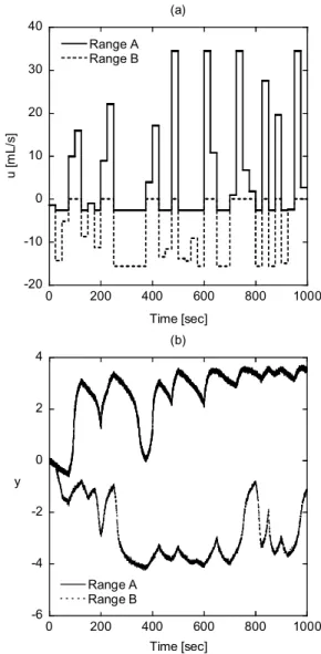
enumerated in Table 1. Figure 1 delineates that the output measurements, y(k), and the effects of initial states and load disturbances,

y

_IL( ),

k

compared against their model predictions, delivered by Eqs. (16) and (19) with n = 3.

It must be pointed out that the true values of process order n

P

, process delay

,and load delay

 are often unknown a priori. To overcome

L

these difficulties, our method yields the optimal estimation of the process model by allowing

, ,

and

 to be secured according to the proposed

_L search procedure with a presumed value of n.

Table 1 reveals that regardless of the occurring time of a load disturbance with distinct dynamics, good process models are obtainable as long as n is set greater than the actual process order n

P

at least by one. Evidently, both settings of n = 4 and n = 3 lead to comparably good estimates of the process model, exact estimates of

 

and rather small values of

J

_OE. A plausible reason is that when the assumed n is greater than n

P

but smaller than the true value, the load delay



_L could be adjusted to account for the unmodeled load dynamics so as to enhance the estimation accuracy. On the contrary, as n is set to 2 (equal to n

P

), the identification results become rather poor as indicated by large values of

J

_OE . It appears that the sole use of

 with no extra

_L time-lag element is unable to describe the behavior of distinct load dynamics. This abrupt change in

J

_OE clearly infers that the actual n

P

is two.

As a further illustration of the effect of n using Case B, Figure 2 compares the actual second load disturbance to the estimated ones obtained by Eq. (11) with

 adjustable. It can be seen

_L that both the estimated load models of n = 4 and 3 approximate well the second load disturbance, whereas the estimated load model of n = 2 fails to describe the load behavior, causing poor estimation of the process model.

Example 2

12.8 18.9 16.7 1 21 1

( ) 6.6 19.4

10.9 1 14.4 1

s s

s

s s

  

   

 

  

   

 

G

P ,

^{1 3}

7 3

 

    δ

, T = 1

This example was investigated by Wood and Berry (1973), which is a two-input/two-output process having various delays. The exact process model with

n

_P,lj = 1 in the z-transform is

0.744 0.879 0.942 0.954 ( ) 0.579 1.302

0.912 0.933

z z

z

z z

  

  

 

  

  

 

GP

The matrices G_P( )

z

and

δ

consist of process elements

G

_P,lj

( ) z

and delay elements

 .

_lj

Assuming t

i

= 0 and N = 300, a test run subject to the measurement noise of NSR = 5% and arbitrarily given initial states were simulated to investigate the effects of deterministic disturbances,

G

_L,1

( ) s

and

G

_L,2

( ), s

on the first and second MISO subsystems:

2 80

L,1 4 5

5 15( 2 1)

( ) (16.7 1)(21 1) ( 1) (5 1) s s e

s

G s

s s s s

 



 

   

80

L,2 2 4

5 15(15 1)

( ) (10.9 1)(14.4 1) (5 1) (30 1) s e

s

G s

s s s s





 

   

The load disturbances with distinct dynamics (

n

_L,1 = 9,

n

_L,2 = 6) entered the system at

L,_l

80.

 

The proposed method based on Eqs. (16), (20), and (21) can arrive at the optimal estimates of process models

G

_{P ,lj}^{( t )} and process delays



_lj

.

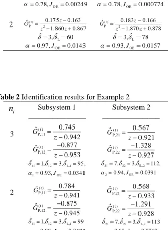
Table 2 lists good identification results for augmented order

n = 3 and acceptable results

_l for

n

_l = 2 acquired by the least-squares estimator

 with the values of

ˆ_N



_l,

 and

_lj

,

 sought. Note that all the estimates of

L ,l

process delays

 are exact. Figure 3 elucidates

_lj that the actual responses of

y k

_l( ) and

y

_IL,l

( ) k

are in excellent agreement with their model predictions obtained using

n

_l = 3. On the contrary, the identification results for

n = 1 (not

_l shown in Table 2) are poor, implying that the actual order of each process unit of G_P( ),

z

P,_lj

,

n

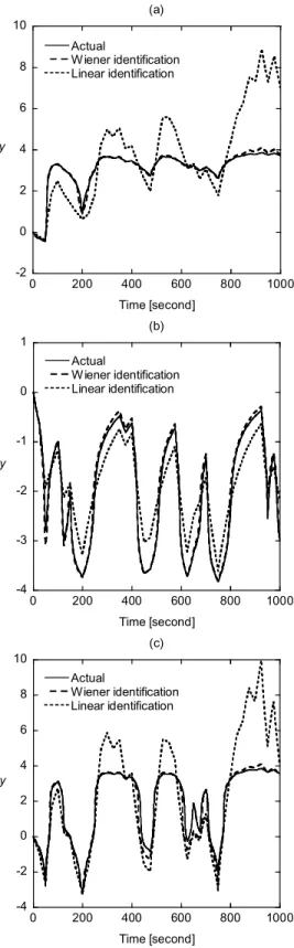
is one.

For stochastic identification, test runs were simulated under arbitrarily assigned initial states and the following load disturbances:

L,1

( ) 8

(16.7 1)(21 1) G s

s s

  

, _L,2

( ) ⁵

(10.9 1)(14.4 1) G s

s s

 

 

Given that

n

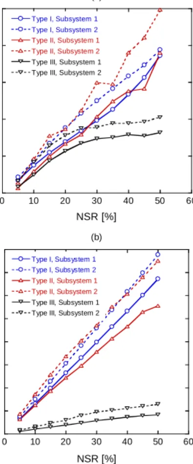
_l 2, n

_F

4, and N = 400, the proposed method is applied to deal with three types of noise characteristics at various levels:

Type I:

G

_V,1

( ) s  1

,

G

_V,2

( ) s  1

Type II: _V,1

( ) ¹ 16.7 1

G s

 s



, _V,2

_{( )} ¹

10.9 1 G s

 s



Type III:

V,1

( ) 1

(16.7 1)(21 1) G s

s s

  

V,2

( ) 1

(10.9 1)(14.4 1) G s

s s

  

Type I disturbance represents measurement noise, whereas type II and type III disturbances represent process noise. The method employs the simplified least-squares estimator and adopts the criterion (29) to infer the best

 value in the

_l face of multifarious noise dynamics. Figure 4 delineates the reliability of the identification results against NSR between 5% and 50% under different noisy conditions. Undoubtedly, the proposed method is excellent in that it yields unbiased and efficient parameter estimates for a wide range of noise level and characteristics.

6. Conclusions

The proposed identification method based on Laguerre models of augmented order is effective in the presence of deterministic and stochastic disturbances under a wide variety of test conditions. The method works well for SISO or MIMO identification involving nonzero initial states as well as load disturbances occurring at unknown time instants during the test. The established error criteria play a crucial role in finding the best time-scaling factor that deals with a wide variety of disturbance characteristics efficiently.

誌謝

本報告內容源於黃世宏與黃宇璋合著之期 刊論文(Huang and Hwang, 2010)以及黃宇璋之 博士論文(Huang, 2010)。

Literature Cited

Hang, C. C., K. J. Åström and W. K. Ho; Automatica, 29, 563-564 (1993).

Huang, Y. C.; PhD Dissertation, National Cheng Kung University (2010).

Huang, Y. C. and S. H. Hwang; J. Chem. Eng. Jpn, 43, 285-295 (2010).

Hwang, S. H. and L. W. Wang; Ind. Eng. Chem. Res., 42, 1905-1913 (2003).

Liu, T. and F. Gao; IEEE Trans. Autom. Control, 53, 2690-2695 (2008).

Park, J. H., S. W. Sung and I. B. Lee; Automatica, 33, 711-715 (1997).

Shen, S. H., J. S. Wu and C. C. Yu; Ind. Eng. Chem.

Res., 35, 1642-1651 (1996).

Wahlberg, B.; IEEE Trans. Autom. Control, 36, 551-

562 (1991).