內容感知的快速運動估計演算法

全文

(1)國立交通大學資訊工程學系碩. 士. 論. 文. 內容感知的快速運動估計演算法 Content-Aware Fast Motion Estimation Algorithm. 研究生：劉祺昱指導教授：李素瑛教授. 中華民國九十四年六月 i.

(2) 內容感知的快速運動估計演算法 Content-Aware Fast Motion Estimation Algorithm. 研究生：劉祺昱. Student: Chi-Yu Liu. 指導教授：李素瑛教授. Advisor: Suh-Yin Lee. 國立交通大學資訊工程學系碩士論文. A Thesis Submitted to Department of Computer Science and Information Engineering College of Electrical Engineering and Computer Science National Chiao-Tung University In partial Fulfillment of the Requirements For the Degree of Master In. Computer Science and Information Engineering. June 2005. Hsinchu, Taiwan, Republic of China. 中華民國九十四年六月 ii.

(3) 內容感知的快速運動估計演算法研究生：劉祺昱. 指導教授：李素瑛教授國立交通大學資訊工程研究所. 摘要在這篇論文中，我們提出內容感知的快速運動估計演算法 (CAFME, Content-Aware Fast Motion Estimation Algorithm) 可以減少運動估計 (Motion Estimation) 所需要的計算量，並且保持幾乎相同的壓縮效率 (Coding Efficiency)。運動估計大致可以分為搜尋 (Search Phase) 與比對 (Matching Phase) 。在搜尋部分，我們基於影片的特性提出動態搜尋範圍演算法 (SDSR, Simple Dynamic Search Range) 以減少需要檢查的搜尋點。在比對部分，我們整合連續排除演算法(SEA, Successive Elimination Algorithm) 與積分影像 (Integral Frame) ，提出一套適合 H.264/AVC 壓縮標準的連續排除演算法。此外，我們以比對誤差 SAD (Sum of Absolute Difference)為量測，提出提前結束演算法 (ETA, Early Termination Algorithm) 。我們所提出的動態搜尋範圍演算法的基本概念是利用運動向量 (Motion Vector) 在空間 (Temporal) 與時間 (Spatial) 的相關性，對目前方塊的搜尋範圍作調整。而我們提出的連續排除演算法則是利用積分影像來計算方塊和 (Block Sum) 且調整原本的連續排除演算法架構，使在運動估計時計算 SAD 的次數可以減少並且重複利用。最後，提前結束演算法則是使用目前方塊預測 SAD 與目前找到最好的 SAD 來衡量運動向量的準確度，以決定是否要結束目前方塊的運動估計。在 H.264/AVC 參考軟體 JM9.4 上實作，實驗結果顯示我們提出的方法所減少的搜尋點可達 93.1%，減少編碼時間大約 42%，而位元率與 PSNR 幾乎相同。. 檢索詞：運動估計、連續排除演算法、積分影像、搜尋範圍、H.264/AVC, SAD, 運動向量. i.

(4) Content-Aware Fast Motion Estimation Algorithm Student: Chi-Yu Liu. Advisor: Prof. Suh-Yin Lee. Department of Computer Science and Information Engineering National Chiao-Tung University. Abstract In this paper, we propose the Content-Aware Fast Motion Estimation Algorithm (CAFME) that reduces computation of motion estimation (ME) while maintains almost the same coding efficiency. Motion estimation can be divided into two phases, searching phase and matching phase. In searching phase, we propose the Simple Dynamic Search Range algorithm (SDSR) based on video characteristics to reduce the number of search points (SP). In matching phase, we integrate the Successive Elimination Algorithm (SEA) and the integral frame to develop a new SEA for H.264/AVC video compression standard, called Successive Elimination Algorithm with Integral Frame (SEAIF). Besides, based on sum of absolute difference (SAD), we also propose the Early Termination Algorithm (ETA) to terminate motion estimation of current block early. The basic idea of Simple Dynamic Search Range algorithm is to adjust the search range of current block by using temporal and spatial correlations of motion vector (MV). Our SEAIF uses “integral frame” to compute block sum and reuses SAD already computed. Finally, the proposed Early Termination Algorithm uses prediction of SAD of current block to measure the accuracy of matching, and then decides to terminate motion estimation or not. We implement in H.264/AVC reference software JM9.4 and the experimental results show that our proposed algorithm can reduce the number of Search Points about 93.1%, encoding time about 42%, while maintains almost the same bitrate and PSNR. Index Terms: motion estimation, successive elimination algorithm, integral frame, search range, H.264/AVC, SAD, motion vector. ii.

(5) Acknowledgement I greatly appreciate the kind guidance of my advisor, Prof. Suh-Yin Lee. In virtue of her graceful suggestions and encouragement, I can complete this thesis. Besides, thanks are extended to all my friends and all the members in the Information System Laboratory for suggestions. I am also grateful to my girl friend because she gives me power and support all the time. Finally, I would like to express my appreciation to my parents for their cares and supports. This thesis is dedicated to them.. iii.

(6) Table of Contents Abstract (Chinese)..................................................................................................................... i Abstract (English) .................................................................................................................... ii Acknowledgement ................................................................................................................... iii Table of Contents..................................................................................................................... iv List of Tables............................................................................................................................ vi List of Figures......................................................................................................................... vii Chapter 1 Introduction............................................................................................................ 1 1.1 Motivation.................................................................................................................... 1 1.2 Related Works .............................................................................................................. 1 1.3 Organization................................................................................................................. 4 Chapter 2 Background Knowledge ........................................................................................ 6 2.1 Block Motion Estimation and Compensation .............................................................. 6 2.2 Matching Criterion....................................................................................................... 7 2.3 Integral Frame .............................................................................................................. 8 2.4 Fast Motion Estimation Algorithms........................................................................... 10 2.4.1 Diamond Search (DS) ......................................................................................11 2.4.2 Successive Elimination Algorithm (SEA)....................................................... 12 2.4.3 Partial Distortion Elimination (PDE).............................................................. 13 2.4.4 Modified Window Follower Algorithm (MWFA) .......................................... 14 Chapter 3 Content-Aware Fast Motion Estimation Algorithm ......................................... 16 3.1 Analysis of Search Range .......................................................................................... 16 3.1.1 Search Range and Frame Rate ........................................................................ 17 3.1.2 Search Range and Frame Resolution .............................................................. 17 3.1.3 Search Range and Motion Activity ................................................................. 18 3.1.4 Search Range, QP, and SAD of Best-matched Block ..................................... 19 3.2 Simple Dynamic Search Range (SDSR).................................................................... 20 iv.

(7) 3.3 Successive Elimination Algorithm with Integral Frame (SEAIF) ............................. 23 3.3.1 Reusing of sea value ....................................................................................... 23 3.3.2 Reusing of SAD value..................................................................................... 24 3.3.3 Spiral Search ................................................................................................... 24 3.3.4 Analysis of complexity ................................................................................... 25 3.4 Early Termination Algorithm (ETA) .......................................................................... 26 Chapter 4 Experimental Results and Discussions............................................................... 30 4.1 Experimental Environment ........................................................................................ 30 4.2 Opponent: Fast Full Pel Search.................................................................................. 32 4.3 Simple Dynamic Search Range.................................................................................. 33 4.4 Successive Elimination Algorithm with Integral Frame ............................................ 37 4.5 Early Termination Algorithm ..................................................................................... 39 4.6 Content-Aware Fast Motion Estimation Algorithm (CAFME).................................. 40 4.7 Summary .................................................................................................................... 42 Chapter 5 Conclusions and Future Works .......................................................................... 44 Bibliography ........................................................................................................................... 45. v.

(8) List of Tables Table 1-1 Advantages and drawbacks of fast motion estimation algorithms ..................... 5 Table 3-1 The relation between SR and FPS ....................................................................... 17 Table 3-2 The relation between SR and resolution ............................................................. 18 Table 3-3 The relation between SR and motion activity..................................................... 18 Table 3-4 The relation between SR, QP, and SAD .............................................................. 19 Table 4-1 Descriptions of test video sequences .................................................................... 31 Table 4-2 Snapshots of test video sequences ........................................................................ 32 Table 4-3 Search Points of FS and SDSR............................................................................. 34 Table 4-4 Bitrates of FS and SDSR....................................................................................... 34 Table 4-5 Total Encoding Time of FS and SDSR................................................................. 35 Table 4-6 Search Points of FS and SEAIF (all block size enabled).................................... 37 Table 4-7 Total Encoding Time of FS and SEAIF (all block size enabled) ....................... 37 Table 4-8 Search Points of FS and SEAIF (16x16 block size only).................................... 38 Table 4-9 Total Encoding Time of FS and SEAIF (16x16 block size only)........................ 38 Table 4-10 SEAIF with different spiral search patterns..................................................... 39 Table 4-11 Search Points of FS and ETA ............................................................................. 39 Table 4-12 Bitrates of FS and ETA ....................................................................................... 40 Table 4-13 Total Encoding Time of FS and ETA................................................................. 40 Table 4-14 Search Points of FS and CAFME ...................................................................... 41 Table 4-15 Bitrates of FS and CAFME ................................................................................ 41 Table 4-16 Total Encoding Time of FS and CAFME .......................................................... 42. vi.

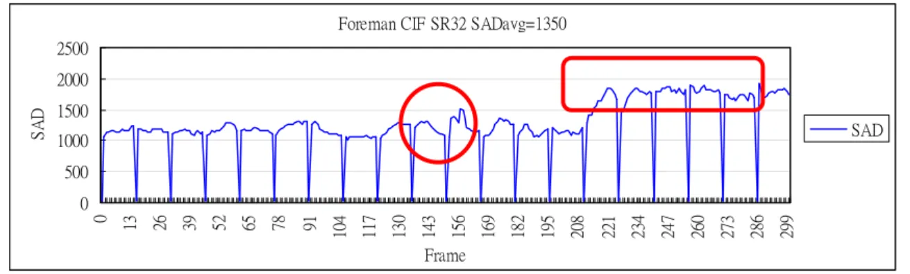
(9) List of Figures Figure 2-1 Motion estimation.................................................................................................. 7 Figure 2-2 Different partition sizes in a macroblock ............................................................ 7 Figure 2-3 Integral frame ........................................................................................................ 9 Figure 2-4 Computation of block sum.................................................................................. 10 Figure 2-5 Diamond search patterns .....................................................................................11 Figure 2-6 Example for search process of Diamond Search .............................................. 12 Figure 3-1 SR and motion activity in foreman QCIF frame by frame.............................. 20 Figure 3-2 SAD of foreman CIF frame by frame ................................................................ 21 Figure 3-3 Current and neighbor blocks (variable block size) .......................................... 22 Figure 3-4 Spiral search in JM 9.4 ....................................................................................... 25 Figure 3-5 Real spiral search pattern................................................................................... 25 Figure 4-1 24th and 25th frame of football CIF sequence .................................................... 36 Figure 4-2 SAD and SR of SDSR frame by frame in Foreman QCIF .............................. 36 Figure 4-3 SAD and SR of SDSR frame by frame in Football CIF................................... 36. vii.

(10) Chapter 1 Introduction 1.1 Motivation Block matching based motion estimation (ME) and compensation is a fundamental process in international video compression standards, such as MPEG-1, MPEG-2, MPEG-4, ITU-T H.263, and H.264, which can efficiently remove temporal redundancy. Since a ME module is usually the most computational intensive part in a typical video encoder (about 50%~90% of the entire system), the efficient ME module is needed. A conventional block-matching algorithm called full search algorithm (FS) exhaustively examines every search point within a search window to find the global optimal matched block in the reference frame. However, FS is too computationally intensive to fit the requirement of real time encoding. Therefore, many fast algorithms have been proposed to alleviate the huge computation of FS. These fast algorithms can be classified into two categories. One is to reduce search points, such as the Three-Step Search (TSS) [1] and Diamond Search (DS) [2]. Another is to simplify the matching operations, such as pixel decimation [3] and SAD-BS measurement [4]. The first category is usually based on the assumption that the MVs are center-biased and the matching error decreases monotonically as the search point moves close to the global minimum position. Since the assumption is often not true in real world videos, these algorithms are often trapped into local minimum. The second category often seriously impairs the accuracy of matching. The algorithms of the two categories suffer for considerable PSNR degradation compared to FS, especially when the motion field is large and complex. Therefore, we would like to propose a new fast algorithm which can avoid local minimum problem and reduce computational cost in matching phase.. 1.2 Related Works In recent years, many fast motion estimation algorithms have been proposed. The Three-Step Search (TSS) [1], New Three-Step Search (NTSS) [4], 2-D Logarithmic Search (2-D LOGS) [6], 1.

(11) Four-Step Search (4SS) [7], Diamond Search (DS) [2], Cross-Diamond Search (CDS) [8] [9] [10], Hexagon-Based Search (HEXBS) [11], Adaptive Rood Pattern Search (ARPS) [12] [13] [14], and Pentagonal Fast Block-Matching Algorithm (PFBMA) [15] are developed to limit the search points to a small subset of all candidate points with certain search pattern. They usually cannot perform well for all kinds of motion activity. Although these algorithms are often trapped into local minimum when motion field is large and complicated, they can considerably reduce the computational cost. Some algorithms like pixel decimation [3] suggest pixel decimation schemes for measuring the block matching based on a set of pixel patterns. SAD-BS [4] partitions a block into sub-blocks and computes the sum of absolute difference (SAD) between the sums of pixel values in the corresponding sub-blocks as the block matching measure. These algorithms determine the tradeoff between accuracy and computational cost in block matching. The Successive Elimination Algorithm (SEA) [16] and Partial Distortion Elimination (PDE) [17] are lossless approaches. The SEA avoids unnecessary SAD calculations by comparing the minimum SAD already found with the absolute difference between the sum of pixel values in current block and the sum of pixel values in candidate block. Due to the advantage of SEA, [18], [19], and [20] are proposed in recent years. The PDE approach uses the partial SAD to eliminate impossible candidates before the complete computation of SAD is performed. The SEA and PDE will perform well when a good candidate point is found at early stage. Because the successive tests will have a tighter distortion bound and may be skipped. Spiral scan order [17] and a good initial MV make more search points be skipped [18]. The Dynamic Search-Window Adjustment (DSWA) [21] adjusts the size of search window in the Three-Step Search (TSS) according to the mean absolute difference (MAD) between current block and candidate block. DSWA compares the first two minimum MADs for each stage of TSS to determine the search direction. The Adaptive Full-Search Block Matching (AFSBM) [22] considers the MAD at the initial search point reflects the degree of motion for a block. Then AFSMB classifies each block into three motion classes by comparing the MAD with thresholds. The two approaches take the block matching error into account for the degree of motion, but there is no 2.

(12) significant correlation between them [23]. The Dynamic Adjustment of Search Window with Variable block size (DASWA) [23] sorts all blocks in a frame according to homogeneity and performs motion estimation for the first block. For the other blocks, the size of search window is set to the magnitude of the MV of adjacent blocks and the search center is set to the position that is pointed to by the MV of adjacent block, which has the largest block similarity. This approach requires the cost of sorting homogeneity and computing similarity. The approach proposed in [24] divides the blocks of a frame into two groups just like chessboard. The blocks in the first groups are motion estimated first. Then the motion estimations for the blocks in second group are performed with dynamic search range depending on the MVs of their neighbor blocks. The Context Adaptive Search (CAS) [25] uses spatial correlation of the motion field and the median predictor. If the median values for both coordinates come from the same macroblock (MB), CAS assumes that motion field is smooth and applies the 3x3 search window. Otherwise, CAS chooses other window size (3x5, 5x3, and 5x5). These approaches only exploit the spatial correlation of motion field. The Window Follower Algorithm (WFA) [26] takes the maximum displacement of MVs in previous frame plus one unit as the size of search window for the current frame. The algorithm fails in the case of sudden motion changes or frames with objects characterized by different motion activities. The modified version of WFA (MWFA) [27] alleviates the problem by exploiting both temporal and spatial correlations in the motion field and adopting the SAD values as a measure of the efficiency of the ME. MWFA needs proper thresholds to measure the accuracy of block matching, however, the thresholds should be determined adaptively by the characteristics of video. The Motion Adaptive Search (MAS) [28] introduces the global motion activity and local motion activity for frame basis and macroblock basis, respectively. Global motion activity uses the mean and variance of the MVs in the previous frame with Chebyshev’s Rule to determine the search range. Then local motion activity adjusts the search range for each MB. In [29], Siou-Shen Lin et al. proposed a motion estimation algorithm with multi-mode by adopting MV variance and SAD threshold. The algorithm changes scheme adaptively according to characteristics of video sequences. 3.

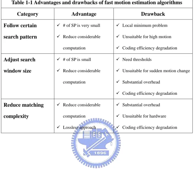
(13) In the previous works, there are some drawbacks such as considerable degradation of PSNR, requirement of appropriate thresholds, substantial overhead, and unsuitable for high motion activity. The drawbacks and advantages of these algorithms are shown in Table 1-1. Because the drawbacks of previous works, we propose the Content-Aware Fast Motion Estimation (CAFME) algorithm to overcome these drawbacks. The CAFME consists of the Simple Dynamic Search Range algorithm (SDSR), Successive Elimination Algorithm with Integral Frame (SEAIF), and Early Termination algorithm (ETA). The SDSR adjusts search range adaptively according to motion activity and performs well regardless of low or high motion. The SEAIF is designed for H.264/AVC visual compression standard and the ETA terminates the search process if the up-to-date block is good enough. Although the CAFME consists of the SDSR, SEAIF, and ETA, these three algorithms can be used independently. The experimental result shows that the proposed SDSR can find a very good search range for each block and maintain almost the same coding efficiency compared with Full Search.. 1.3 Organization The paper is organized as follows. Chapter 2 introduces the related background knowledge, including motion estimation, integral frame, and related algorithms. In Chapter 3, we present how the Content-Aware Fast Motion Estimation Algorithm is designed and developed. Chapter 4 reports the significant experimental results. Finally, the conclusions and future works are given in Chapter 5.. 4.

(14) Table 1-1 Advantages and drawbacks of fast motion estimation algorithms Category. Advantage. Drawback. Follow certain. # of SP is very small. Local minimum problem. search pattern. Reduce considerable. Unsuitable for high motion. computation. Coding efficiency degradation. Adjust search. # of SP is small. Need thresholds. window size. Reduce considerable. Unsuitable for sudden motion change. computation. Substantial overhead Coding efficiency degradation. Reduce matching. Reduce considerable. Substantial overhead. complexity. computation. Unsuitable for hardware. Lossless approach. Coding efficiency degradation. 5.

(15) Chapter 2 Background Knowledge In this chapter, we introduce some background knowledge related to our proposed approaches. At first, we acquaint you with block motion estimation and compensation. Second, matching criterions for motion estimation are described briefly. Next, integral frame is presented. Finally, some fast motion estimation algorithms are presented in detail.. 2.1 Block Motion Estimation and Compensation Motion estimation and compensation techniques are used to remove temporal redundancy of inter frames. An ideal approach is to segment the frame into some objects including moving and stationary objects. However, the segmentation of objects is difficult and impractical. A practical and widely used method of motion compensation is to compensate for movement of blocks of the currents frame. We call this method as block-based motion estimation and compensation. Usually the block is a 16x16-pixel region of a frame, called macroblock (MB). The MB is the basic unit for motion compensated prediction in many of visual coding standards including MPEG-1, MEEG-2, MPEG-4, H.263 and H.264. Motion estimation of a macroblock involves finding a 16x16-pixel block in a reference frame that closely matches the current macroblock. The reference frame may be before or after the current frame in display order. An area in the reference frame centered on the search center is searched and the 16x16-pixel block within the search area that minimizes the matching criterion is chosen as the best-matched block. The height and width of the search area are considered as the size of search window as shown in Figure 2-1.. 6.

(16) Reference frame. Current frame. Best matched block. Current MB MV. Search range Figure 2-1 Motion estimation. The new visual coding standard H.264/AVC introduces the overlapped variable block size to improve coding efficiency. There are seven block sizes, 16x16, 16x8, 8x16, 8x8, 8x4, 4x8, and 4x4, forming the following partitions of a 16x16 macroblock as depicted in Figure 2-2. When P8x8 type is considered, the 8x8, 8x4, 4x8, and 4x4 type must be considered for each of the four individual 8x8 sub-blocks. Note that each partition has its own unique motion vector [30].. 16×16 type. 16×8 type. 8×8 type. 8x4 type. 8×16 type. 4x8 type. P8×8 type. 4x4 type. Different partition sizes for a macroblock subtype in P8×8 mode. Figure 2-2 Different partition sizes in a macroblock. 2.2 Matching Criterion In order to choose the best-matched block, a matching criterion is needed. Mean square 7.

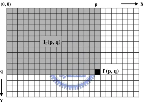
(17) difference (MSD), mean absolute difference (MAD), and sum of absolute difference (SAD) are frequently used criterions. Their definitions can be described by the following equations.. 1 MN. MSD( fc, fr (m, n)) = MAD ( fc, fr (m, n)) =. 1 MN. M −1 N −1. ∑ ∑ ( f (i, j) − f (i + m, j + n) ) c. 2. r. (2.1). i =0 j =0. M −1 N −1. ∑∑. fc(i, j ) − fr (i + m, j + n). (2.2). i =0 j =0. M −1 N −1. SAD( fc, fr (m, n)) = ∑ ∑ fc(i, j ) − fr (i + m, j + n). (2.3). i =0 j =0. M and N is the width and height of the block, respectively. m and n are horizontal and vertical component of motion vector, respectively. fc and fr are the current and reference blocks, respectively. MSD, MAD, and SAD have very high accuracy in block matching. However, SAD does not need any multiplication operations. Therefore, SAD is the most popular criterion used in the international video coding standards. Unlike other video coding standards, H.264 uses the Lagrange multiplier to compute the rate distortion cost for each partition within a macroblock. The best-matched block is selected by minimizing the following Lagrange cost.. J ( MV , λ motion) = SAD ( fc, fr (m, n )) + λ motion ⋅ Rate( MV − MVP ). (2.4). MV = (m, n) is the motion vector, MVP = (mPx, nP) is the prediction for motion vector, andλ motion. is the Lagrange multiplier. The function Rate(MV－MVP) represents the predicted motion. error and is implemented by a look up table [31].. 2.3 Integral Frame In this section, we introduce integral frame technique which is used in our Successive Elimination Algorithm (SEA) to compute the sum of pixel values in a block efficiently. We denote the sum of pixel values in a block as block sum (BS). Viola et al. [31] proposed the integral frame 8.

(18) technique for sum of pixel values within any rectangular area in a frame. Given a video frame f, the value of its integral frame at pixel (p, q) is denoted as If (p, q), as defined in the equation (2.5).. p. q. If ( p, q ) = ∑∑ f (i, j ). (2.5). i = 0 j =0. The integral frame is shown in Figure 2-3. (0, 0). p. X. If (p, q). f (p, q). q. Y. Figure 2-3 Integral frame. The computational cost for an integral frame is described as follows. Let Rf (p, q) be the cumulative row sum of pixel values in frame f. The definitions are:. p. Rf ( p, q) = ∑ f (i, q ). (2.6). i =0. Rf (-1, q ) = 0 If ( p, -1) = 0 Rf ( p, q ) = Rf ( p − 1, q ) + f ( p, q) If ( p, q ) = If ( p, q − 1) + Rf ( p, q ). (2.7) (2.8) (2.9) (2.10) 9.

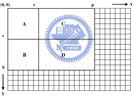
(19) By using equation (2.9) and (2.10) recursively, one can compute the integral frame If in one pass. For a frame with W x H pixels, 2WH additions are required to compute an integral frame. The sum of pixel values in any rectangular block in a frame can be computed by three arithmetic operations. For example, as illustrated in Figure 2-4, the BS of block D can be computed by equation (2.11).. BS ( D) =. p. q. ∑∑. f (i, j ) = If ( p, q) − If (r , q ) − If ( p, s ) + If ( r , s ). (2.11). i = r +1 j = s +1. (0, 0). r. p. A. C. B. D. X. s. q. Y. Figure 2-4 Computation of block sum. 2.4 Fast Motion Estimation Algorithms In this section, we introduce some fast motion estimation algorithms, including Diamond Search [2], Successive Elimination Algorithm [16], Partial Distortion Elimination [17], and modified Window Follower Algorithm [27].. 10.

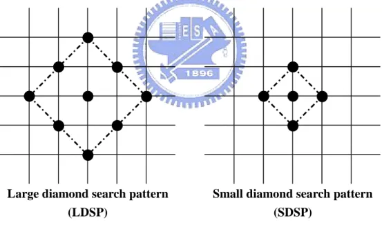
(20) 2.4.1 Diamond Search (DS) Just as other conventional fast motion estimation algorithms, DS [2] is also designed to reduce the number of search points in motion estimation. DS has very good performance compared with the Three-Step Search (TSS), New Three-Step Search (NTSS), and Four-Step Search (4SS). However, DS are still often trapped into local minimum problem. DS employs two search patterns in motion estimation, as illustrated in Figure 2-5. The first pattern called large diamond search pattern (LDSP) is repeatedly used until the step in which the minimum block distortion occurs at the center point. After that, the second pattern called small diamond search pattern (SDSP) is used as the final step. The minimum block distortion point found in SDSP is the final solution of MV, which points to the best -matched block. See Figure 2-6 for example of search process.. Large diamond search pattern. Small diamond search pattern. (LDSP). (SDSP). Figure 2-5 Diamond search patterns. 11.

(21) -6. -5. -4. -3. -2. -1. 0. 1. 2. 3. 4. 5. 6. 7. -6 -5 -4 -3 -2 -1 0 1 2 3 4 5 6. Figure 2-6 Example for search process of Diamond Search. 2.4.2 Successive Elimination Algorithm (SEA) In motion estimation, the SAD of each block in the search window is compared with the current minimum SAD. If the SAD of the current block is smaller than the current minimum SAD, the block is considered as up-to-date best-matched block. In order to reduce the computation of SAD, Successive Elimination Algorithm (SEA) [16] was proposed. The SEA is a lossless fast motion estimation algorithm based on mathematical inequality. The main idea of SEA can be shown in the equation (2.12).. M −1 N −1. SAD( fc, fr (m, n)) = ∑ ∑ fc(i, j ) − fr (i + m, j + n) i =0 j =0. ≥. M −1 N −1. ∑∑ i =0 j =0. M −1 N −1. fc (i, j ) − ∑ ∑ fr (i + m, j + n). (2.12). i =0 j =0. ≡ BSc − BSr (m, n) ≡ sea( fc, fr (m, n)). In equation (2.12), BSc and BSr are the block sums in the current block and candidate block, 12.

(22) respectively. Because SAD(fc, fr(m, n)) is equal to or larger than sea(fc, fr(m, n)), if sea(fc, fr(m, n)) is larger than the current minimum SAD, SAD(fc, fr(m, n)) must be larger than the current minimum SAD. Therefore, computation of SAD(fc, fr(m, n)) can be skipped. To compute sea value is easier than to compute SAD, because BSc has to be calculated only once and BSr(m, n) can be derived from the previous value of BSr(m－1, n). Hence, SEA can reduce the computation of SAD efficiently. Multilevel SEA (MSEA) proposed in [20] is a generalized SEA. MSEA divides a macroblock into sub-blocks and calculates the BS for each sub-block. Then we compute the sum of absolute differences of the corresponding BSs as mesa(fc, fr(m, n)). The mesa(fc, fr(m, n)) is always equal to or larger than sea(fc, fr(m, n)). Consequently, the mesa(fc, fr(m, n)) is a lower bound of SAD. The equation (2.13) describes the idea.. M −1 N −1. SAD( fc, fr (m, n)) = ∑ ∑ fc(i, j ) − fr (i + m, j + n) i =0 j =0. ≥. 22 L −1. ∑. BSck − BSrk (m, n). k =0. ≡ msea ( fc, fr (m, n)). (2.13). ≥ BSc − BSr (m, n) ≡ sea( fc, fr (m, n)). In Equation (2.13), k is the index of sub-block and L is the level of division. For example, when N=16 and M=16, msea with level L=0 is reduced to sea, and msea with level L=4 is the same as SAD. Obviously, the bound is lower when the level is higher; however, the computational cost is higher.. 2.4.3 Partial Distortion Elimination (PDE) The concept of PDE [17] uses the partial sum of difference to eliminate impossible candidates before the complete calculation of SAD. The basic concept is shown in equation (2.14).. 13.

(23) M −1 k −1. SADk ( fc, fr (m, n)) = ∑ ∑ fc (i, j ) − fr (i + m, j + n) ≥ SAD( fc, fr (m, n)). (2.14). i =0 j =0. In the process of computation of SAD, we compute the partial SAD and compare the partial SAD with the current minimum SAD. If the partial SAD is equal to or larger than the current minimum SAD, the calculation of SAD can be terminated and the search point can be skipped. Owing to the overhead of testing inequality, the testing is performed every row. Like SEA, if we can find a smaller SAD early, the more candidates can be skipped.. 2.4.4 Modified Window Follower Algorithm (MWFA) Window follower algorithm (WFA) [26] takes the maximum displacement of MV in previous frame plus one unit as the search range for the current frame. The algorithm is presented as follows.. Window Follower Algorithm [27]. Step 1: For the kth frame, compute the maximum horizontal and vertical displacement from all. MVs in (k－1)th frame. The maximum value D is defined as equation (2.15). The dt represents the maximum displacement of two components of MV of tth block.. D = max[dt ]. (2.15). dt = max ⎢⎣ MVtx, MVty ⎥⎦. (2.16). Step 2: Perform motion estimation for kth frame with search range P=D+1. For the first frame, the. search range P is set to max search range.. 14.

(24) WFA assumes that [26]: (1) The change of motion content between frames is gradual and not sudden. (2) The motion content is constant over a large number of successive frames. However, the characteristics of motion in natural video sequences are various and hardly predictable. The assumptions of WFA may not be true in natural video sequences. MWFA [27] modifies WFA by exploiting both temporal and spatial information and adopting SAD as a measure of accuracy of MV. MWFA algorithm is presented as follows.. Modified Window Follower Algorithm [28]. Step 1: For the kth frame, compute the displacement D as defined in WFA. Step 2: Perform motion estimation for each block in kth frame with search range Pt, for tth block. Pt. is determined by the following mutually exclusive rules. (1) If (SADmint-1 >= TH1). Pt = Pmax, F = 1. (2) If (SADmint-1 <= TH1 and F == 1) Pt = max (D, d t-1) + 1 If (SADmint-1 <= TH1 and F == 0) Pt = D + 1 (3) If (SADmint-1 <= TH2 and F == 1) Pt = max (D, d t-1) If (SADmint-1 <= TH2 and F == 0) Pt = D. SADmint-1 and d t-1 represent the minimum SAD and the maximum MV displacement for the (t －1)th block in the current frame, respectively. The flag F is set to zero at the beginning of each. frame. When the flag F is set to zero, only temporal information is considered; when the flag F is set to one, both temporal and spatial information are taken into account. The threshold TH1 and TH2 are set to 4096 and 2048, respectively, derived from simulations of typical video sequences.. 15.

(25) Chapter 3 Content-Aware Fast Motion Estimation Algorithm In this chapter, we present our proposed Content-Aware Fast Motion Estimation Algorithm (CAFME), which consists of SDSR, SEAIF, and ETA. At first, section 3.1 presents some observations and analyses of search range in motion estimation. Simple dynamic search range algorithm (SDSR) and SEA with integral frame (SEAIF) are presented in section 3.2 and 3.3, respectively. Finally, our early termination algorithm (ETA) is given in section 3.4.. 3.1 Analysis of Search Range In this section, we want to explore the relationships among the parameters in the motion estimation. Because adjustment of search range needs some information, the relationships can help us to develop a good algorithm. We did some experiments to observe and analyze the relationships between search range (SR) and frame rate, frame resolution, motion activity, quantization parameter (QP), and SAD of best-matched block. The experimental environment is as follows. Platform: H.264/AVC reference software JM 9.4 [32] Machine: Athlon XP 1700+ with 512 MB memory Profile: baseline Level: 3.0 Block match algorithm (BMA): full search Group of picture (GOP): 15 Frame structure: IPPP Number of reference frame: 1 Hadamard transform: enable All block size (16x16, 16x8, 8x16, 8x8, 8x4, 4x8, and 4x4): enable Rate-distortion optimized (RDO): enable Fast ME (UMHexagonS) [33]: disable Fast mode selection [34]: disable 16.

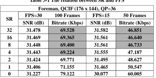
(26) Rate control (RC): disable 16x16 MB observed. 3.1.1 Search Range and Frame Rate Since the frame rate affects the difference of successive frames, so we observe the relationship between SR and frame rate. The test data are foreman sequence with FPS=30 and FPS=15. The temporal distance of sequence with FPS=30 is 1/30 second and the temporal distance of sequence with FPS=15 is 1/15 second. In theory, when the frame rate is higher, the motion estimation needs smaller search range. The Quantization parameter (QP) is mapped into quantization step and affects the bitrate significantly. In our experiments, the QP is fixed and RC is disabled. Therefore, we only need to observe the bitrate field for different search ranges. In Table 3-1, the gray areas represent the bitrates are stable and the search ranges are enough to find true MVs in motion estimation. We can observe that the bitrates are approximately stable when the SR≧4 with FPS=30 and the SR≧8 with FPS=15. Experimental results show a larger search range is required to find the true MV when the frame rate is lower. The experimental results conform to the theory.. Table 3-1 The relation between SR and FPS. SR 32 16 8 4 2 1 0. Foreman, QCIF (176 x 144), QP=36 FPS=30 100 Frames FPS=15 50 Frames SNR (dB) Bitrate (Kbps) SNR (dB) Bitrate (Kbps) 31.478 69.528 31.582 46.851 31.469 69.365 31.561 46.640 31.448 69.400 31.561 46.733 31.443 69.224 31.555 47.187 31.424 69.771 31.495 48.627 31.406 71.155 31.465 50.547 31.227 79.122 30.077 60.005. 3.1.2 Search Range and Frame Resolution We test the coastguard sequence in QCIF and CIF resolution. In Table 3-2, the gray areas in 17.

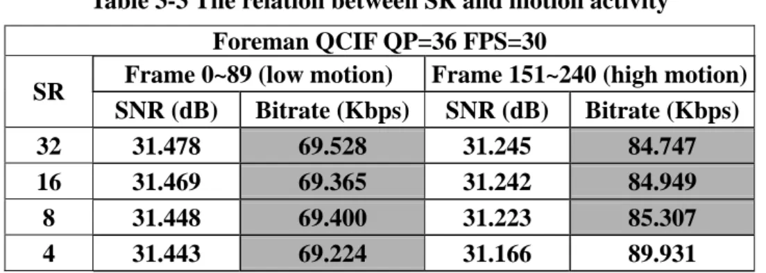
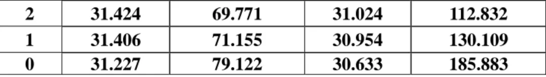
(27) QCIF resolution represent the bitrates change slightly when the SR is from 2 to 32 and the gray areas in CIF resolution represent the bitrates change slightly when the SR is from 4 to 32. These observations present the SR≧2 is large enough to find the true MVs in QCIF resolution and SR≧4 is large enough to find the true MVs in CIF resolution. Therefore we conclude that the search range is required to increase adaptively for the larger resolution.. Table 3-2 The relation between SR and resolution. SR 32 16 8 4 2 1 0. Coastguard, QP=36, FPS=30, Encoded frames=90 QCIF (176 x 144) CIF (352 x 288) SNR (dB) Bitrate (Kbps) SNR (dB) Bitrate (Kbps) 29.178 71.992 29.315 375.003 29.183 72.304 29.312 375.539 29.185 72.325 29.299 374.728 29.168 71.747 29.289 376.667 29.144 72.520 29.271 387.957 29.107 76.120 29.225 420.099 28.799 113.893 28.920 639.923. 3.1.3 Search Range and Motion Activity We divide the foreman sequence into two parts, which represent the low and high motion sequences. The first part consists of first 90 frames and the second part consists of frames from frame 151 to 240. In Table 3-3, we observe that the bitrates are approximately stable when the SR ≧4 in low motion sequence and the SR≧8 in high motion sequence. As we expect, the search. range should be increased adaptively for high motion sequences.. Table 3-3 The relation between SR and motion activity. SR 32 16 8 4. Foreman QCIF QP=36 FPS=30 Frame 0~89 (low motion) Frame 151~240 (high motion) SNR (dB) Bitrate (Kbps) SNR (dB) Bitrate (Kbps) 31.478 69.528 31.245 84.747 31.469 69.365 31.242 84.949 31.448 69.400 31.223 85.307 31.443 69.224 31.166 89.931 18.

(28) 2 1 0. 31.424 31.406 31.227. 69.771 71.155 79.122. 31.024 30.954 30.633. 112.832 130.109 185.883. 3.1.4 Search Range, QP, and SAD of Best-matched Block In block matching, SAD is used as matching criterion. If SR is too small, then the true MV may not be found and the SAD found at the best-matched block will be large. Besides, the QP also affects SAD obviously. Therefore, this experiment considers these factors. In Table 3-4, the field SAD best average means the average of SAD value causes the minimum rate distortion cost in H.264/AVC encoder. The experimental result shows the true MVs can be found as long as SR≧8 regardless of QP while QP only affects the magnitude of SAD. We also show the SAD best average frame by frame in Figure 3-1. In foreman sequence, the motion is higher than the rest of the sequence from frame 150 to 220. Therefore, SR≦4 is not large enough to find the true MVs.. Table 3-4 The relation between SR, QP, and SAD Foreman QCIF 300 Frames FPS=30 SAD best average QP=18 QP=24 QP=30 921.2 1024.0 1221.3 924.7 1027.8 1226.0 942.9 1045.6 1244.6 1068.8 1165.5 1353.8 1252.9 1344.9 1524.4 1413.7 1503.7 1585.9 1831.9 1911.4 2081.7. SR 32 16 8 4 2 1 0. QP=36 1577.5 1584.9 1605.3 1702.9 1860.9 2001.9 2330.1. Foreman QCIF QP36 4000. SR4 SR32. 2000 1000. Frame. 19. 299. 286. 273. 260. 247. 234. 221. 208. 195. 182. 169. 156. 143. 130. 117. 104. 91. 78. 65. 52. 39. 26. 13. 0 0. SAD. 3000.

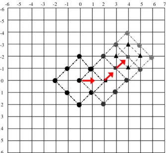
(29) Figure 3-1 SR and motion activity in foreman QCIF frame by frame. In Summary, if we can find a SR for a frame or a block in motion estimation such that the true MVs can be found, the local minimum problem can be avoided and the computational cost of motion estimation can be reduced dramatically. In our experiments, the search range should be changed adaptively according to motion activity of video and parameters of encoder. However, the parameters of encoder should be used by comparing with each other. Hence, we develop SDSR to adjust SR dynamically based on motion activity.. 3.2 Simple Dynamic Search Range (SDSR) In this section, we present our proposed Simple Dynamic Search Range algorithm (SDSR). In order to adjust search range for motion estimation, some approaches have already been implemented in DSWA [21], AFSBM [22], MWFA [27], and MAS [28]. These approaches may be classified into block matching error based and motion vector based. The block matching error is usually measured in MSD, MAD or SAD. The block matching error represents the degree of matching between current block and candidate block. The value of block matching error is determined by many factors including motion activity, texture, and quantization parameter. See Figure 3-2 for example. From frame 220, the values of SAD are much higher than the rest. The reason is the complicated video texture, not the motion activity. However, from frame 150 to 170, the values of SAD are raised sharply due to the sudden motion change instead of video texture. Consequently, the approaches based on block matching error are usually unsuitable to evaluate the motion activity. On the contrary, motion vector represents the motion activity more precisely [28]. For this reason, our proposed approach is based on motion vector information. Due to the wide variations of motion activity in video sequences and different motion activity in various areas within a single frame, we would like to adjust search range on both frame level and block level. The adjustments of SR in frame level and block level are based on temporal correlation and spatial correlation of 20.

(30) motion field, respectively.. Foreman CIF SR32 SADavg=1350 2500. SAD. 2000 1500 SAD. 1000 500 299. 286. 273. 260. 247. 234. 221. 208. 195. 182. 169. 156. 143. 130. 117. 104. 91. 78. 65. 52. 39. 26. 13. 0. 0 Frame. Figure 3-2 SAD of foreman CIF frame by frame. The proposed Simple Dynamic Search Range algorithm is described as follows. Simple Dynamic Search Range Algorithm. Step 1: Determine the search range in frame level. The search range called SR_FRAMEk is. computed by the maximum horizontal and vertical displacement from all MVs in (k－1)th frame plus one unit. The definition is:. SR _ FRAMEk = max[ MVxt , MVyt ] + 1. (3.1). t ∈ {all blocks in (k -1)th frame}. Step 2: Adjust the search range in macroblock level. Let MV_MAXt denote the maximum. displacement of two components of MVs in neighbor blocks of tth block, described as in the following rules. s ∈ ﹛The left, above left, above, above right blocks of tth block﹜ If any of neighbor blocks is not available. MV _ MAXt = max[max[ MVxs, MVys ], SR _ FRAMEk ] Else. 21.

(31) MV _ MAXt = max[ MVxs, MVys ]. Step 3: Determine the final search range for tth block, called SR_BLOCKt by the following rules.. //Adjust SR in block level If ( MV _ MAXt ≥ SR _ FRAMEk ) SR _ BLOCKt = MV _ MAXt + 1 Else SR _ BLOCKt = MV _ MAXt + ( SR _ FRAMEk − MV _ MAXt ) / 2 //SR constraint If ( SR _ BLOCKt ≤ 1) SR _ BLOCKt = 1 Else if ( SR _ BLOCKt ≥ max search range) SR _ BLOCKt = max search range. Because the prediction of MV may not be zero MV in motion estimation, the displacement of MV may be larger than the SR. Hence the SR in frame level may increase more than one unit between frames. The adjustment of SR in block level ensures that the SR is large enough to find the true MV. Note that the neighbor block of current block may not be a complete macroblock (16x16) in H.264/AVC video compression standard, shown in Figure 3-3.. C D (8x4). (16x8). B (8x4). A (8x8). E (16x16). Figure 3-3 Current and neighbor blocks (variable block size). 22.

(32) 3.3 Successive Elimination Algorithm with Integral Frame (SEAIF) The SEA and integral frame technique had been introduced in section 2.4.2 and 2.3. In this section, we integrate them to form a new SEA called SEAIF for H.264/ACV standard. In H.264/AVC standard, rate-distortion optimization (RDO) is recommended for mode selection. The modes include nine intra modes and seven inter modes (see Figure 2-2). In inter-coding, a total of 41 motion estimations is required for a 16x16 macroblock while the RDO is enabled. (One for 16x16, two for 16x8, two for 8x16, four for 8x8, eight for 8x4, eight for 4x8, and sixteen for 4x4) Therefore, the ME cost increases dramatically. In order to reduce the intensive computation caused by RDO. In the H.264/AVC reference software JM 9.4 [32], a Fast Full Pel Search algorithm is implemented by reusing SAD values of the smallest 4x4 block. Before a new macroblock is motion estimated, it computes the SAD values for all 4x4 block at all search points within the search window. After that, it merges the SAD values to get the SAD values of larger blocks. In this way, computation of SAD for a macroblock with all block size enabled is about equal to the computation of SAD with only a 16x16 block. We take the concept of reusing SAD and integrate it into our proposed SEAIF. The main idea of the SEAIF for H.264/AVC is to reuse sea values and SAD values. The following sub-sections present the detail of the design. Section 3.3.1 and 3.3.2 present the techniques of reusing sea and SAD values. Section 3.3.3 presents the spiral search pattern used by SEAIF algorithm. Finally, analysis of complexity for SEAIF is presented in Section 3.3.4.. 3.3.1 Reusing of sea value For each search point, calculate the sea values of sixteen 4x4 blocks of the current macroblock by using integral frame technique. These sea values of 4x4 blocks are the basis for sea values of larger blocks. Then the sea values of larger blocks are derived from these sea values of 4x4 blocks, described as follows.. For 8x4 or 4x8 block, sum up sea values of two 4x4 blocks. 23.

(33) For 8x8 block, sum up sea values of two 8x4 blocks. For 16x8 or 8x16 block, sum up sea values of two 8x8 blocks. For 16x16 block, sum up sea values of two 16x8 blocks.. In this way, we can get all sea values of all blocks. These sea values of larger blocks are always equal to or larger than the sea values computed directly from BS of corresponding blocks. Therefore, the sea values of larger blocks derived from 4x4 block sea values are lower bound of SAD and the more computations of SAD can be skipped.. 3.3.2 Reusing of SAD value In SEAIF, if the sea value is less than the current minimum SAD value, complete calculation of SAD will be preformed. In H.264/AVC, overlapped blocks are used in motion estimation. In order to reduce the computations of SAD, we take the 4x4 block SAD values as the basis of the larger block SAD values. The following is the approach.. Reusing SAD value algorithm. Regardless of block size, Calculation of SAD for the block is: Step1: Find out all 4x4 blocks within the block. Step2: Check the SAD values of these 4x4 blocks. If any SAD value of 4x4 blocks is not available,. compute the SAD value. Step3: Get the SAD value of the target block by adding up SAD values of these 4x4 blocks.. In this way, there is no redundant computation of SAD.. 3.3.3 Spiral Search In JM 9.4, the spiral search for full search is not really spiral shape. Therefore, we modified it. 24.

(34) to the real spiral shape shown in Figure 3-4 and Figure 3-5, respectively. Chapter 4 will show the experimental results for comparisons.. 49 35 37 39 41 43 45 47 …. 25 15 17 19 21 23 26. 27 9 3 5 7 10 28. 29 11 1 0 2 12 30. 31 13 4 6 8 14 32. 33 16 18 20 22 24 34. 49 48 47 46 45 44 43 42. 36 38 40 42 44 46 48. Figure 3-4 Spiral search in JM 9.4. … 25 24 23 22 21 20 41. 26 9 8 7 6 19 40. 27 10 1 0 5 18 39. 28 11 2 3 4 17 38. 29 12 13 14 15 16 37. 30 31 32 33 34 35 36. Figure 3-5 Real spiral search pattern. 3.3.4 Analysis of complexity The reason of adopting SEA is to reduce the computational cost in block matching measurement. The overhead of SEA should be considered and analyzed. The overheads of SEA are mainly the computations of block sum. In SEA [16], Salari et al. proposed a fast algorithm to compute the block sums. We compare three approaches and present the analysis of overhead as follows. Let W denote image width, H image height, M block width, and N block height. Operations required for block sums of all M x N blocks in a reference frame are:. Straightforward approach:. Number of block sum in a frame: (W－M + 1)(H－N + 1) Operations required for a block sum: MN－1 Total cost: (MN－1) (W－M + 1)(H－N + 1) Approximate cost: MNWH. SEA approach in [16]:. Total cost: 4WH－(H－N)(M + 3)－3W(N + 1) 25.

(35) Approximate cost: 4WH. Integral frame approach:. Operations required for an integral frame: 2WH Operations required for all block sum: ≈ 2(W－M + 1)(H－N + 1) 1 Total cost: 2WH + 2(W－M + 1)(H－N + 1) Approximate cost: 4WH. Although integral frame approach and the SEA approach in [16] have approximately the same complexity, there is an advantage in integral frame approach. Integral frame approach is flexible to get block sum of any rectangle block. For example, if we want to use the multilevel SEA for each block size in H.264/AVC, the implementation will be easier with integral frame approach. (Note that our approach uses the tighter lower bound in SEA, not multilevel SEA.) Computing msea value of 16x16 block with level L=0 only needs 5 operations (5 = 3 for get BS + 1 subtraction + 1 absolute). Nevertheless, merging 16 4x4 sea values to get the sea value of 16x16 block with level L=0 needs 15 addition operations while the sea value is tighter lower bound. Trade-off is between the tighter lower bound and computational complexity.. 3.4 Early Termination Algorithm (ETA) In this section, we preset our proposed Early Termination Algorithm (ETA) in detail. In [29], Siou-Shen Lin et al. introduce the variance of motion vectors. They show the probability is about 79% in average when the variance of the current block and neighbor blocks is smaller than 3. They consider that it is high probability that the current block and the neighbor blocks might belong to the same object when the variance of the motion vectors in the neighbor blocks is small. We exploit and modify the variance of motion vectors proposed in [29] to classify the motion. 1. In [4], Viet Anh Nguyen and Yap-Pen Tan proposed a fast approach to calculate block sum by exploiting the adjacent property of the blocks. 26.

(36) activity of current block and neighbor blocks into simple motion and complex motion. The variance of motion vectors is defined in equation (3.3).. MVmean = ( MVa + MVb + MVc + MVd ) / 4. (3.2). MVvar = MVa − MVmean + MVb − MVmean + MVc − MVmean + MVd − MVmean. (3.3). If any of neighbor blocks is not available, MVvar is set to a large value (999999). For accuracy, we compare the MVvar with 5 instead of 3 to classify motion activity, shown in equation (3.4).. If (MVvar ≦ 5) Mactivity = simple_motion. (3.4). Else Mactivity = complex_motion. If motion activity is simple motion, we consider the current block and neighbor blocks are in the same object for simple. On the contrary, the current block and neighbor blocks are considered not in the same block. The SAD values of blocks within the same object should be similar and the SAD values of blocks not in the same object should be different largely. Based on the concept, the lower bound for the condition of termination is determined in equation (3.5).. If (Mactivity == simple_motion) SAD_threshold = SAD_prediction. (3.5). Else SAD_threshold = SAD_prediction – SAD_standard_deviatoin. The SAD_prediction and SAD_standard_deviation represent the prediction of SAD of current block and the standard deviation of SAD of all blocks in the previous frame, respectively. The definitions are defined in equation (3.6) and (3.8):. 27.

(37) SAD_prediction = ( SADa + SADb + SADc + SADd ) / 4. SAD_mean =. (3.6). Number _ MB −1 1 SADt ∑ Number _ MB t =0. (3.7). 1/ 2. ⎛ 1 M −1 2⎞ SAD_standard_deviatoin = ⎜ ( SADt − SAD_mean ) ⎟ ∑ ⎝ M − 1 t =0 ⎠. (3.8). The SADt is the SAD value of tth block in a frame. Number_MB is the total number of MB in a frame. If there is no any neighbor block near the current block, SAD_prediction is set to a small value (-999999). Note that the SAD_prediction and SAD_standard_deviation are calculated for 16x16 macroblock. In H.264/AVC standard, there are seven block sizes used in motion estimation. We determine the SAD_prediction and SAD_standard_deviation for other block size according to the area occupied by the block. The calculations are shown in the following rules. Adjustment of SAD_prediction and SAD_variance for H.264/AVC standard. If (block size == 16x8 or 8x16) SAD_prediction = SAD_prediction / 2 SAD_standard_deviation = SAD_standard_deviation / 2 Else if (block size == 8x8) SAD_prediction = SAD_prediction / 4 SAD_standard_deviation = SAD_standard_deviation / 4 Else if (block size == 8x4 or 4x8) SAD_prediction = SAD_prediction / 8 SAD_standard_deviation = SAD_standard_deviation / 8 Else if (block size == 4x4) SAD_prediction = SAD_prediction / 16 SAD_standard_deviation = SAD_standard_deviation / 16. 28.

(38) Finally, the condition of termination is tested when a new up-to-date best-matched block is found. If the SAD value of the up-to-date block is equal to or smaller than SAD_threshold, the motion estimation is terminated.. 29.

(39) Chapter 4 Experimental Results and Discussions In this chapter, we present the experimental results of the proposed approaches including simple dynamic search range algorithm, successive elimination algorithm with integral frame, and early termination algorithm. Finally, the experimental results of integrated algorithm called Content-Aware Fast Motion Estimation Algorithm (CAFME) are presented. We modify the H.264/AVC reference software JM 9.4 and implement the proposed algorithms on it. In the experiments, we compare the proposed algorithm with Full Search (FS). We observe the number of search points for each block to measure the performance of the proposed algorithms. We also measure the coding efficiency. In order to measure the coding efficiency, we compare the bitrates of encoded sequences with the same quantization parameter and disabling rate control. Besides, we exploit the SAD value as a criterion to measure whether the determined search range is large enough. Finally, we compare the total encoding time to measure the improvement in practical situation.. 4.1 Experimental Environment In this section, we present the experimental environment. The descriptions and snapshots of test video sequences are listed in Table 4-1 and Table 4-2, respectively. Except specifically described parameters, the following parameters are applied to all experiments. Note that the maximum search range is set to 24. Platform: H.264/AVC reference software JM 9.4 [32] Machine: Athlon XP 1700+ with 512 MB memory Profile: baseline Level: 3.0 Block match algorithm (BMA): Full Search Group of picture (GOP): 15 Quantization parameter (QP): 36 30.

(40) Frame rate (FPS): 30 Max search range: 24 Frame structure: IPPP Number of reference frame: 1 Hadamard transform: enable All block size (16x16, 16x8, 8x16, 8x8, 8x4, 4x8, and 4x4): enable Rate-distortion optimized (RDO): enable Fast ME (UMHexagonS) [33]: disable Fast mode selection [34]: disable Rate control (RC): disable. Table 4-1 Descriptions of test video sequences. ID. Name. Resolution. # of Frames. Motion activity. A. Foreman. QCIF. 150. Medium. B. Mobile. QCIF. 150. Slow. C. Coastguard. QCIF. 150. Medium. D. Foreman. CIF. 150. Medium. E. Tempete. CIF. 150. Slow, Zooming. F. Flower. CIF. 90. Slow. G. Stefan. SIF. 150. High. H. Football. CIF. 90. Very High. I. Table tennis. SIF. 90. Medium, Scene change, Zooming. 31.

(41) Table 4-2 Snapshots of test video sequences. Foreman QCIF. Mobile QCIF. Coastguard QCIF. Foreman CIF. Tempete CIF. Flower CIF. Stefan SIF. Football CIF. Table tennis SIF. 4.2 Opponent: Fast Full Pel Search In our experiments, we compare our proposed algorithms with Fast Full Pel Search2. The Fast Full Pel Search is implemented by reusing SAD values of the smallest 4x4 block. Before a new macroblock is motion estimated, it computes the SAD values for all 4x4 block at all search points within the search window. After that, it merges the SAD values to get the SAD values of larger 2. The Fast Full Pel Search is implemented in H.264/AVC Reference Software JM 9.4 32.

(42) blocks. In this way, computation of SAD for a macroblock with all block size enabled is about equal to the computation of SAD with only a 16x16 block. Note that the performances of the Fast Full Pel Search and a conventional Full Search are the same but the Fast Full Pel Search is faster than a conventional Full Search in H.264/AVC. In the following experiments, we denote the Fast Full Pel Search as FS.. 4.3 Simple Dynamic Search Range In this section, we experiment on nine sequences with our proposed Simple Dynamic Search Range (SDSR). The nine test sequences include the various motion activities. In Table 4-3, the proposed SDSR outperforms the Fast Full Pel Search (FS) greatly. For the low and medium motions, SDSR reduces the number of search points about 77% ~ 98%. For the high motion, SDSR reduces the size of search window much less reasonably. For example, the reduced rate is 41% for Football sequence which represents the high motion activity. In Table 4-4, we can observe that the bitrates increases slightly, except Football sequence. In the Table 4-5, the total encoding time is reduced about 40~50%, except Stefan and Football sequences. The motion activity of Stefan and Football sequences are higher than others. The Figure 4-1 presents the two successive frames of Football sequence for illustration. In order to measure whether the search ranges determined by the SDSR is large enough. We depict Figure 4-2 and Figure 4-3 to present the measurement. The Figure 4-2 is the average SAD values frame by frame in Foreman QCIF sequence with SDSR and FS. We can observe the SAD values of SDSR and FS are very similar. This observation shows that SDSR can find true MVs in most of the motion estimations. The Figure 4-3 is the average SAD values frame by frame in Football CIF sequence with SDSR and FS. We can observe the differences between SAD values of SDSR and FFS are larger in some frames because the motion activities are much higher. In average, the number of search points is reduced about 80%, bit rate increases about 0.11%, and total encoding time is reduced about 43%. Hence, we claim the proposed SDSR can keep almost the same coding efficiency.. 33.

(43) Table 4-3 Search Points of FFS and SDSR. Number of Search Points Sequence Name. Improvement Fast Full Pel Search. SDSR. Foreman QCIF. 2401. 144. － 94%. Mobile QCIF. 2401. 52. － 98%. Coastguard QCIF. 2401. 88. － 96%. Foreman CIF. 2401. 365. － 85%. Tempete CIF. 2401. 261. － 89%. Flower CIF. 2401. 563. － 77%. Stefan SIF. 2401. 860. － 64%. Football CIF. 2401. 1411. － 41%. Table tennis SIF. 2401. 497. － 79% － 80%. Average. Table 4-4 Bitrates of FS and SDSR. Bitrates (Kbps) Sequence Name. Improvement Fast Full Pel Search. SDSR. Foreman QCIF. 69.203. 68.858. － 0.5%. Mobile QCIF. 173.016. 173.250. ＋ 0.1%. Coastguard QCIF. 76.134. 76.022. － 0.1%. Foreman CIF. 188.773. 188.490. － 0.1%. Tempete CIF. 425.392. 425.810. ＋ 0.1%. Flower CIF. 669.312. 669.333. ＋ 0.003%. Stefan SIF. 505.450. 505.693. ＋ 0.05%. Football CIF. 413.301. 416.525. ＋ 0.8%. Table tennis SIF. 256.259. 257.925. ＋ 0.65% ＋ 0.11%. Average 34.

(44) Table 4-5 Total Encoding Time of Fast Full Pel Search and SDSR. Total Encoding Time (Second) Sequence Name. Improvement Fast Full Pel Search. SDSR. Foreman QCIF. 156. 74. － 53%. Mobile QCIF. 151. 75. － 50%. Coastguard QCIF. 151. 70. － 54%. Foreman CIF. 602. 319. － 47%. Tempete CIF. 583. 324. － 44%. Flower CIF. 374. 221. － 41%. Stefan SIF. 508. 340. － 33%. Football CIF. 363. 280. － 23%. Table tennis SIF. 298. 169. － 43% － 43%. Average. 35.

(45) Figure 4-1 24th and 25th frame of football CIF sequence. Figure 4-2 SAD and SR of SDSR frame by frame in Foreman QCIF. Figure 4-3 SAD and SR of SDSR frame by frame in Football CIF. 36.

(46) 4.4 Successive Elimination Algorithm with Integral Frame In Table 4-6 and Table 4-7, SEAIF reduces the number of search points about 76%, while the total encoding time increases about 14% in average. The reason is the overlapped block used in H.264/AVC standard. When SEAIF is applied for overlapped blocks, the condition of computing SAD is tested more than once for the same area. Hence, the probability of computing SAD rises, and then the computational cost of calculation of SAD cannot be reduced largely. In addition to the overhead of SEAIF, the encoding time is more slightly. In Table 4-8 and Table 4-9, only 16x16 block size is enabled for motion estimation. There is no overlapped block. Therefore, the performance of SEAIF is better and the encoding time is less.. Table 4-6 Search Points of FS and SEAIF (all block size enabled). Number of Search Points Sequence Name. Improvement Fast Full Pel Search. SEAIF. Foreman QCIF. 2401. 491. － 80%. Mobile QCIF. 2401. 553. － 77%. Tempete CIF. 2401. 584. － 76%. Stefan SIF. 2401. 669. － 72% － 76%. Average. Table 4-7 Total Encoding Time of Fast Full Pel Search and SEAIF (all block size enabled). Total Encoding Time (Second) Sequence Name. Improvement Fast Full Pel Search. SEAIF. Foreman QCIF. 156. 157. ＋ 0.64%. Mobile QCIF. 151. 172. ＋ 14%. Tempete CIF. 583. 690. ＋ 18%. Stefan SIF. 508. 579. ＋ 14%. 37.

(47) ＋ 12%. Average. Table 4-8 Search Points of FS and SEAIF (16x16 block size only). Number of Search Points Sequence Name. Improvement Fast Full Pel Search. SEAIF. Foreman QCIF. 2401. 61. － 97%. Mobile QCIF. 2401. 71. － 97%. Tempete CIF. 2401. 114. － 95%. Stefan SIF. 2401. 193. － 92% － 95%. Average. Table 4-9 Total Encoding Time of Fast Full Pel Search and SEAIF (16x16 block size only). Total Encoding Time (Second) Sequence Name. Improvement Fast Full Pel Search. SEAIF. Foreman QCIF. 112. 77. － 31%. Mobile QCIF. 117. 84. － 28%. Tempete CIF. 458. 332. － 28%. Stefan SIF. 369. 289. － 27% － 29%. Average. In the section 3.3.3, we modified the spiral search pattern in JM 9.4. The experimental result is presented in Table 4-10. Although the search patterns are different, all the search points are examined. The best-matched blocks with the same RD cost may not be the same due to the different search order. Therefore, the results in bitrate field are slightly different. The effects of both patterns are almost the same, so we use the spiral search pattern in JM 9.4 with our proposed SEAIF.. 38.

(48) Table 4-10 SEAIF with different spiral search patterns. Bitrate (Kbps). Total Encoding Time (Sec). Sequence Name JM 9.4. Ours. Improvement. JM 9.4. Ours. Improvement. Foreman QCIF. 69.203. 68.981. ＋0.3%. 157. 155. －1.3%. Mobile QCIF. 173.016. 173.413. ＋0.2%. 172. 167. －2.9%. Tempete CIF. 425.392. 425.678. ＋0.07%. 690. 649. －5.9%. Stefan SIF. 505.450. 505.566. ＋0.02%. 579. 546. －5.7%. ＋0.15%. Average. －3.95%. 4.5 Early Termination Algorithm In Table 4-11, Table 4-12, and Table 4-13, our proposed Early Termination Algorithm (ETA) reduces the number of SP about 44.5% and the bit rate is nearly the same with FS. However, the encoding time is not reduced as we expect. In motion estimation, each search point is estimated in matching criterion, usually SAD. The proposed ETA terminates the searching process early to reduce the computations of SAD. In this experiment, our ETA is used with the Fast Full Pel Search algorithm3 and the algorithm calculates all SAD values in advance. Although our ETA can skip a large number of search points, it can not save the computations of SAD. So the encoding time can not be saved in this experiment. The proposed Early Termination Algorithm should be used with other algorithms instead of the algorithms computing SAD in advance.. Table 4-11 Search Points of FS and ETA. Number of Search Points Sequence Name. 3. Improvement Fast Full Pel Search. ETA. Foreman QCIF. 2401. 1484. － 38%. Mobile QCIF. 2401. 1197. － 50%. The algorithm is proposed in H.264/AVC reference software JM9.4. 39.

(49) Tempete CIF. 2401. 1306. － 46%. Stefan SIF. 2401. 1350. － 44% － 44.5%. Average. Table 4-12 Bitrates of FS and ETA. Bitrates (Kbps) Sequence Name. Improvement Fast Full Pel Search. ETA. Foreman QCIF. 69.203. 69.365. ＋ 0.2%. Mobile QCIF. 173.016. 173.366. ＋ 0.2%. Tempete CIF. 425.392. 424.898. － 0.1%. Stefan SIF. 505.450. 505.987. ＋ 0.1% ＋ 0.1%. Average. Table 4-13 Total Encoding Time of Fast Full Pel Search and ETA. Total Encoding Time (Second) Sequence Name. Improvement Fast Full Pel Search. ETA. Foreman QCIF. 156. 140. － 10.3%. Mobile QCIF. 151. 152. ＋ 0.7%. Tempete CIF. 583. 594. ＋ 1.9%. Stefan SIF. 508. 498. － 2.0% － 2.4%. Average. 4.6 Content-Aware Fast Motion Estimation Algorithm (CAFME) In this section, we integrate the simple dynamic search range (SDSR), successive elimination algorithm with integral frame (SEAIF), and early termination algorithm (ETA) to form the Content-Aware Fast Motion Estimation Algorithm (CAFME). In the Table 4-14, Table 4-15, and Table 4-16, the number of search points can be reduced. 40.

(50) more than 90% in most of the sequences. Especially, for the slow and median motion, the reduced rates of search points are about 99%. For high motion, the reduced rates of search points should be lower. The reduced rate of search points is 73.8% for football sequence. In average, the increment of bit rate in CAFME is very small, about 0.26%. The total encoding time is reduced about 41.9%, and the number of SP is reduced about 93.1%.. Table 4-14 Search Points of FS and CAFME. Number of Search Points Sequence Name. Improvement Fast Full Pel Search. CAFME. Foreman QCIF. 2401. 37. － 98.5%. Mobile QCIF. 2401. 12. － 99.5%. Coastguard QCIF. 2401. 29. － 98.8%. Foreman CIF. 2401. 100. － 95.8%. Tempete CIF. 2401. 69. － 97.1%. Flower CIF. 2401. 199. － 91.7%. Stefan SIF. 2401. 184. － 92.3%. Football CIF. 2401. 628. － 73.8%. Table tennis SIF. 2401. 224. － 90.7% － 93.1%. Average. Table 4-15 Bitrates of FS and CAFME. Bitrates (Kbps) Sequence Name. Improvement Fast Full Pel Search. CAFME. Foreman QCIF. 69.203. 69.118. － 0.12%. Mobile QCIF. 173.016. 173.285. ＋ 0.16%. Coastguard QCIF. 76.134. 75.862. － 0.36%. Foreman CIF. 188.773. 188.784. ＋ 0.005%. 41.

(51) Tempete CIF. 425.392. 425.955. ＋ 0.13%. Flower CIF. 669.312. 670.211. ＋ 0.13%. Stefan SIF. 505.450. 504.782. － 0.13%. Football CIF. 413.301. 419.357. ＋ 1.5%. Table tennis SIF. 256.259. 258.939. ＋ 1.04% ＋ 0.26%. Average. Table 4-16 Total Encoding Time of Fast Full Pel Search and CAFME. Total Encoding Time (Second) Sequence Name. Improvement Fast Full Pel Search. CAFME. Foreman QCIF. 156. 69. － 56%. Mobile QCIF. 151. 77. － 49%. Coastguard QCIF. 151. 68. － 55%. Foreman CIF. 602. 314. － 48%. Tempete CIF. 583. 318. － 45%. Flower CIF. 374. 224. － 40%. Stefan SIF. 508. 324. － 36%. Football CIF. 363. 325. － 10%. Table tennis SIF. 298. 184. － 38% － 41.9%. Average. 4.7 Summary The proposed Simple Dynamic Search Range (SDSR) can reduce the number of search points about 80% while sustaining the coding efficiency (bitrate increases 0.11% in average). We also integrate the Successive Elimination Algorithm with Integral Frame (SEAIF) and the Early Termination Algorithm (ETA) with SDSR to form the Content-Aware Fast Motion Estimation Algorithm (CAFME). The CAFME improves the SDSR and the number of search points is reduced. 42.

(52) to 93.1% while the bit rate increases just a little (0.26%). The overall encoding time is reduced about 41.9% in our implementation.. 43.

(53) Chapter 5 Conclusions and Future Works The motion estimation plays an important role in the video compression. However, motion estimation module is usually the most computational intensive part in a typical video encoder. Hence, the efficient motion estimation algorithm is needed. We proposed a fast algorithm called Content-Aware Fast Motion Estimation Algorithm (CAFME). CAFME consists of the Simple Dynamic Search Range (SDSR), Successive Elimination Algorithm with Integral Frame (SEAIF), and Early Termination Algorithm (ETA). The SDSR adjusts the search range for every block adaptively. The SEAIF reduces the number of computation of SAD without loss. The ETA terminates the search process early when finding a good candidate block. The SDSR need not predefined any threshold predefined and perform well for all the test sequences. The SEAIF is designed for overlapped variable block size and applies reusing techniques. The performance of ETA is good and stable for all kinds of motion activity. The experimental results show that CAFME can reduce the number of search point about 93.1% and the bitrate only increases 0.26% while sustaining the same PSNR. We modify H.264/AVC reference software JM 9.4 and implement our proposed algorithms on it. The total encoding time reduces about 41.9%. The motion search algorithm currently used in CAFME is full search (FS). However it may be replaced by any fast motion estimation algorithm like TSS and DS, etc. The future works may be to develop a fast motion estimation algorithm suitable for dynamic search range, alleviate the overhead in implementation, and so on.. 44.

(54) Bibliography [1]. T. Koga, K. Iinuma, A. Hirano, Y. Iijima, and T. Ishiguro, “Motion Compensated Interframe Coding for Video Conferencing” Proc. Nat. Telecommun. Conf., pp. G5.3.1–5.3.5, New Orleans, LA, Nov. 29–Dec. 3 1981.. [2]. S. Zhu and K.-K. Ma, “A New Diamond Search Algorithm for Fast Block-Matching Motion Estimation”, IEEE Trans. on Image Processing, Volume 9, Issue 2, pp. 287–290, Feb. 2000.. [3]. B. Liu and A. Zaccarin, “New Fast Algorithms for the Estimation of Block Motion Vectors”, IEEE Trans. on Circuits System Video Technology, Volume 3, pp. 148–157, Apr. 1993.. [4]. V.-A. Nguyen and Y.-P. Tan, “Fast Block-Based Motion Estimation Using Integral Frames”, IEEE Signal Processing Letters, Volume 11, Issue 9, pp. 744–747, Sep. 2004.. [5]. R. Li, B. Zeng, and M.-L. Liou, “A New Three-Step Search Algorithm for Block Motion Estimation”, IEEE Trans. on Circuits and Systems for Video Technology, Volume 4, Issue 4, pp. 438–442, Aug. 1994.. [6]. J. Jain and A. Jain, “Displacement Measurement and Its Application in Interframe Image Coding” IEEE Trans. on Communications, Volume COMM-29, pp. 1799–1808, Dec. 1981.. [7]. L.-M. Po and W.-C. Ma, “A Novel Four-Step Search Algorithm for Fast Block Motion Estimation” IEEE Trans. on Circuits and Systems for Video Technology, Volume 6, Issue 3, pp. 313–317, Jun. 1996.. [8]. C.-H. Cheung and L.-M. Po, “A Novel Cross-Diamond Search Algorithm for Fast Block Motion Estimation” IEEE Trans. on Circuits and Systems for Video Technology, Volume 12, Issue 12, pp. 1168–1177, Dec. 2002.. [9]. C.-W. Lam, L.-M. Po, and C.-H. Cheung, “A New Cross-Diamond Search Algorithm for Fast Block Matching Motion Estimation” 2003 International Conf. on Neural Networks and Signal Processing, Volume 2, pp. 1262-1265, Dec. 14-17 2003.. [10] H. Jia and L. Zhang, ”A New Cross Diamond Search Algorithm for Block Motion Estimation” Proc. of IEEE International Conf. on Acoustics, Speech, and Signal Processing, Volume 3, pp. iii-357-60, May 17-21 2004. 45.

(55) [11] C. Zhu, X. Lin, L. Chau, and L.-M. Po, “Enhanced Hexagonal Search for Fast Block Motion Estimation” IEEE Trans. on Circuits and Systems for Video Technology, Volume 14, Issue 10, pp. 1210–1214, Oct. 2004. [12] Y. Nie and K.-K. Ma, “Adaptive Rood Pattern Search for Fast Block-matching motion estimation” IEEE Trans. on Image Processing, Volume 11, Issue 12, pp. 1442–1449, Dec. 2002. [13] K.-K. Ma and G. Qiu, “Unequal-Arm Adaptive Rood Pattern Search for Fast Block-Matching Motion Estimation in the JVT/H.26L” 2003 International Conf. on Image Processing, Volume 1, pp. I-901-4, Sep. 14-17 2003. [14] K.-K. Ma and G. Qiu, “An Improved Adaptive Rood Pattern Search for Fast Block-Matching Motion Estimation in JVT/H.26L” Proc. of the 2003 International Symposium on Circuits and Systems, Volume 2, pp. II-708 - II-711, 25-28 May 2003. [15] Y.-C. Lim, K.-Y. Min, and J.-W. Chong, “A Pentagonal Fast Block Matching Algorithm for Motion Estimation Using Adaptive Search Range” IEEE International Conf. on Acoustics, Speech, and Signal Processing, Volume 3, pp. III - 669-72, Apr. 6-10 2003. [16] W. Li and E. Salari, “Successive Elimination Algorithm for Motion Estimation” IEEE Trans. on Image Processing, Volume 4, Issue 1, pp. 105–107, Jan. 1995. [17] Digital Video Coding Group, ITU-T Recommendation H.263 Software Implementation, Telenor R&D, 1995. [18] M. Yang, H. Cui, and K. Tang, “Efficient Tree Structured Motion Estimation Using Successive Elimination” IEE Proc. on Vision, Image and Signal Processing, Volume 151, Issue 5, pp. 369–377, Oct. 30 2004. [19] Yu-Wen Huang, Shao-Yi Chien, Bing-Yu Hsieh, and Liang-Gee Chen, “Global Elimination Algorithm and Architecture Design for Fast Block Matching Motion Estimation” IEEE Trans. on Circuits and Systems for Video Technology, Volume 14, Issue 6, pp. 898–907, Jun. 2004. [20] X.Q. Gao, C.J. Duanmu, and C.R. Zou, “A Multilevel Successive Elimination Algorithm for Block Matching Motion Estimation” IEEE Trans. on Image Processing, Volume 9, Issue 3, pp. 501–504, Mar. 2000. 46.