類別結構的亂度因素、刺激向度個數對分類學習行為的影響 - 政大學術集成

全文

(1)國立政治大學心理學系研究所碩士學位論文. 指導教授楊立行博士. 立. 政治大. ‧ 國. 學. 類別結構的亂度因素、刺激向度個數對分類學習行為的影響. ‧. category learning. n. al. er. io. sit. y. Nat. Categorical entropy, number of stimulus dimensions, and. Ch. engchi. i n U. 研究生林家源撰. 101 年 6 月. v.

(2) Contents 中文摘要.................................................................................................................................... 1 Abstract ...................................................................................................................................... 2 Literature Reviews ..................................................................................................................... 3 Past theories of categorization ........................................................................................... 4 Learning condition of categorization ............................................................................... 12 Category structures .......................................................................................................... 13 Sloutsky’s dual systems theory ........................................................................................ 15 Statistical density ............................................................................................................. 18 Incongruent evidence with Sloustky’s dual systems theory ............................................ 22 Methods.................................................................................................................................... 28 Experiment 1 .................................................................................................................... 28 Apparatus ................................................................................................................. 28 Participants ............................................................................................................... 29 Stimulus ................................................................................................................... 29 Procedure ................................................................................................................. 33 Results ...................................................................................................................... 34 Experiment 2 .................................................................................................................... 37 Participants ............................................................................................................... 37 Stimulus ................................................................................................................... 38 Procedure ................................................................................................................. 41 Results ...................................................................................................................... 41. 立. 政治大. ‧. ‧ 國. 學. n. er. io. sit. y. Nat. al. i n U. v. Experiment 3 .................................................................................................................... 44 Participants ............................................................................................................... 45 Stimulus ................................................................................................................... 45 Procedure ................................................................................................................. 47 Results ...................................................................................................................... 47 General Discussions ................................................................................................................. 52 Study Restrictions ............................................................................................................ 53 Statistical Density ............................................................................................................ 56 Multiple Systems for Category Learning ......................................................................... 57 Dimensionality of Materials ............................................................................................ 59 Base rate of categories ..................................................................................................... 61 Conclusion ............................................................................................................................... 62 Reference ................................................................................................................................. 63 Appendix .................................................................................................................................. 70 Examples of calculating statistical density ...................................................................... 70. Ch. engchi.

(3) Running head: Materials dimensionality and category learning. 中文摘要 Sloutsky (2010; Kloos 與 Sloutsky, 2008) 操弄不同的類別結構亂度 (categorical entropy) 進行類別學習作業，藉此提出了雙系統理論，認為人們會啟動不同的系統，濃縮式系統 (compression-based system)或選擇式系統 (selection-based system)，以適應不同的類別結構組成之刺激材料。本研究回顧了 Sloutsky 的研究證據與過去類別學習領域的相關文獻，認為此雙系統理論可能只適用在向度數目較多的情境之下，因此設計了三個實驗，使用. 政治大. 和 Kloos 與 Sloutsky (2008) 相同的實驗派典，欲說明刺激材料的向度個數確實會影響到. 立. 人們的類別學習行為。實驗一發現，Sloutsky 所預測的類別結構與學習方式之交互作用. ‧ 國. 學. 只出現在向度個數較多的情境，向度個數少時則無此交互作用。實驗二得到與實驗一相. ‧. 同的結果，並排除了刺激材料本身特性（幾何圖形或類自然類別材料）此一混淆變項。. y. Nat. al. er. io. sit. 實驗三採用特別設計的依變項，直接觀察受試者採用相似性(similarity)或規則(rule)的方. v. n. 式進行分類判斷，集群分析的結果顯示在向度數目少的情境時，不管何種類別結構受試. Ch. engchi. i n U. 者均傾向使用以規則為基礎的選擇式系統學習。因此，綜合以上發現，本研究認為 Sloutsky 的雙系統理論必須考慮到向度數目此一變項，才能更廣泛的應用於各種類別學習情境之中。. 1.

(4) Running head: Materials dimensionality and category learning. Abstract The goal of this research is to point out that the dimensions of experimental materials can influence human category learning, which is neglected by traditional models of category learning. Three experiments in this research examined the effect of stimuli dimensionality by following the paradigms of Kloos and Sloutsky (2008). In Experiment 1, the prediction of Sloutsky’s theory (2010) on the interaction effect between category structures and learning conditions succeeds only at high dimensionality of materials, but fails in the low. 政治大 dimensionality condition. Experiment 2 was conducted by the same experimental setting as 立. ‧ 國. 學. Experiment 1, but the natural-like stimuli were replaced by well-defined artificial geometrics. The result of Experiment 2 is the same as Experiment 1, suggesting that the dimensionality of. ‧. sit. y. Nat. materials plays a critical role in category learning no matter what kind of stimuli are used.. n. al. er. io. Experiment 3 found that various materials dimensionality had distinct effects on human. Ch. i n U. v. category representations. Namely, when experimental stimuli are relatively complex, people. engchi. would use the corresponding category learning system to represent stimuli to learn dense categories or sparse ones. In contrast, when the stimuli are relatively simple, participants would represent the stimuli in a rule-based manner both in dense and sparse category structures.. 2.

(5) Running head: Materials dimensionality and category learning. Literature Reviews Categorization plays a crucial role in cognitive psychology, and numerous researches focus on how category learning performance is influenced by various category structures and learning conditions (Alfonso-Reese, Ashby, and Brainard, 2002; Ashby, Maddox, and Bohil, 2002; Ashby, Queller, and Berretty, 1999; Colreavy & Lewandowsky, 2008; Kruschke, 1993; Love, 2002; Shepard, Hovland, and Jenkins, 1961). Specifically, researchers focus on. 政治大. developing models to account for the type of mental representations and the process for. 立. categorization, which people use/generate in category learning (Ashby & Gott, 1988; Ashby,. ‧ 國. 學. Alfonso-Reese, Turken, & Waldron, 1998; Erickson & Kruschke, 1998; Kruschke, 1992;. ‧. Medin & Smith, 1981; Nosofsky, 1986). For instance, the generalized context model (GCM). y. Nat. al. er. io. sit. is developed by the idea of storing every exemplar into mental memory space (Nosofsky,. v. n. 1986), whereas the general recognition theory assumes that classification behaviors are. Ch. engchi. i n U. determined by learning decision boundaries (Ashby & Gott, 1988). In contrast to single system theories, Sloutsky (2010) proposed a dual systems theory which posits that two systems, the selection-based system and the compression-based system are employed for learning categories of different “statistical density”. The index “statistical density” was developed in Sloutsky’s studies (Kloos & Sloutsky, 2008; Sloutsky, 2010) in order to represent the characteristics of category structure. A category structure composed of multi-dimensional exemplars can be simply described by the calculation of statistical density 3.

(6) Running head: Materials dimensionality and category learning. as simple figures ranging from 0 to 1. In addition, the statistical density indicates the regularity of category structure. Namely, a high level of density represents the category structure in high regularity. However, category structures maybe oversimplified by this index, for instance, some researchers suggest that the dimensionality of materials could influence participants’ learning strategies and category perceptions (Livingstion, Andrews, and Harnad, 1998; Minda & Smith, 2001; Nosofsky, Stanton, and Zaki, 2005; Verguts, Ameel, and Storms,. 政治大. 2004). Therefore, the present study suggests that Sloutsky’s dual systems theory should be. 立. re-organized with assessing the effects of materials dimensionality. This thesis is organized in. ‧ 國. 學. the order of reviewing relevant categorization theories, re-examining Sloutsky’s theory,. Nat. y. ‧. showing the experiment results, and providing general discussions.. er. io. sit. Past theories of categorization. The classic theory of Aristotle is known as the oldest theory of categorization. This. n. al. Ch. engchi. i n U. v. theory assumes that an exemplar would belong to a specific category only if it has all features required by this category. For example, a square is defined as a closure figure which has four equal sides and four vertical angles. Therefore, a closure figure is a square if it has all features mentioned above (Smith & Medin, 1981). The closure figure with four equal sides and four vertical angles is definitely a square. This is so-called a “well-defined” stimulus where there is a condition of sufficient and necessary relation between item features and the concept of a category (Martin & Caramazza, 1980). 4.

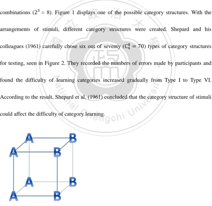
(7) Running head: Materials dimensionality and category learning. However, learning a category is more than learning the sufficient and necessary relations between the stimulus feature and the concept of category. Shepard, Hovland and Jenkins (1961) revealed that the human learning performance is influenced a lot by category structure. In their study, each stimulus could be defined by its size, shape, and color. For each dimension, there were two levels (e.g., the figure could be either triangle or square, either black or white, and either big or small). Therefore, there would be eight stimuli for all the. 政治大. combinations (23 = 8). Figure 1 displays one of the possible category structures. With the. 立. arrangements of stimuli, different category structures were created. Shepard and his. ‧ 國. 學. ‧. colleagues (1961) carefully chose six out of seventy (C48 = 70) types of category structures. for testing, seen in Figure 2. They recorded the numbers of errors made by participants and. Nat. io. sit. y. found the difficulty of learning categories increased gradually from Type I to Type VI.. n. al. er. According to the result, Shepard et al. (1961) concluded that the category structure of stimuli. Ch. engchi. could affect the difficulty of category learning.. i n U. v. Figure 1. Example of category structure. Two categories are labeled as “A” and “B”. 5.

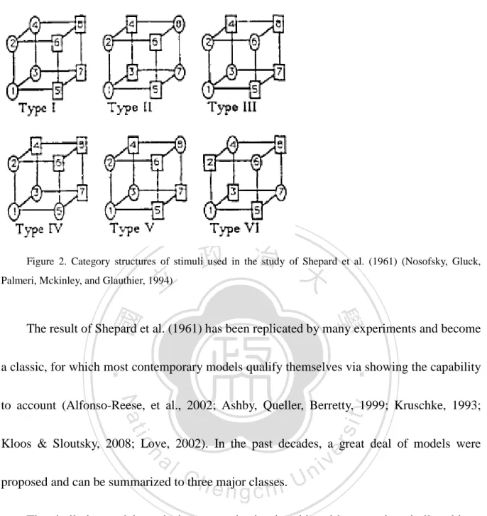
(8) Running head: Materials dimensionality and category learning. 政治大. Figure 2. Category structures of stimuli used in the study of Shepard et al. (1961) (Nosofsky, Gluck,. 立. Palmeri, Mckinley, and Glauthier, 1994). ‧ 國. 學. The result of Shepard et al. (1961) has been replicated by many experiments and become. ‧. a classic, for which most contemporary models qualify themselves via showing the capability. Nat. io. sit. y. to account (Alfonso-Reese, et al., 2002; Ashby, Queller, Berretty, 1999; Kruschke, 1993;. n. al. er. Kloos & Sloutsky, 2008; Love, 2002). In the past decades, a great deal of models were. Ch. engchi. proposed and can be summarized to three major classes.. i n U. v. The similarity models posit that categorization is achieved by grouping similar objects together and by separating apart those dissimilar ones. Both the prototype and exemplar-based models are belonged to this class. Different from the classic theory of Aristotle, the main idea of prototype theory comes from the attempt to address categorization of natural objects instead of artificial items. It indicates that there are “natural prototypes” of concepts (Rosch, 1973). For example, when referring to a bird, the first idea comes to our 6.

(9) Running head: Materials dimensionality and category learning. mind may be a sparrow, but not a chicken nor a penguin. It suggests that a sparrow is more typical than a chicken when the concept of birds is mentioned. In this way, the relation between the features of exemplars and the concepts of a category is not sufficient and necessary. In other words, a bird may have some typical features like wings, feathers, being able to fly in the sky, and so on, but not every creature is categorized as a “bird” which has all features above. These kinds of stimuli are called ‘ill-defined’, which means the boundary of a. 政治大. concept cannot be clearly described (McCloskey & Glucksberg, 1978). There are. 立. idiosyncratic features in some exemplars (like penguin is a bird which cannot fly), while the. ‧ 國. 學. core features of a concept are the mostly appeared (like every bird has feathers). Therefore,. ‧. an exemplar with core features was the prototype of concept (Homa & Chambliss, 1975). In. Nat. io. sit. y. other words, the prototype is always the most typical exemplar of a category. This is unlike. n. al. er. the classic theory, which assumes the representatives of each exemplar to a category concept are all the same.. Ch. engchi. i n U. v. The prototype model claims that people would compare a new stimulus to the most typical exemplars of a category, the prototype, when they need to do classification. The new stimulus would be classified as the same category if it is similar to the prototype, otherwise it would be classified as a different category. Similar to the prototype model, the exemplar-based model posits that people would compare to a new stimulus to every exemplar, not the prototype only, in the categories and 7.

(10) Running head: Materials dimensionality and category learning. classify it as the category with a relatively high similarity (e.g., context model; Medin & Schaffer, 1978; GCM (generalized context model); Nosofsky, 1984, 1986, 1987). Following the influential exemplar-based model, GCM, the similarity is derived from the negative exponential transformation of the distance between items in the psychological space. The probability of classifying Stimulus i to Category CJ can be illustrated by P�R J �Si� = ∑m. 𝑏J ∑j∈CJ ηij. K=1(𝑏K ∑k∈CK ηik ). Equation 1-1. 政治大. where 𝑏J represents the bias for making response R J and the index “j ∈ CJ ” means that. 立. ‧ 國. 學. similarity between Si and each Sj belonging to CJ should be calculated. The ηij which is. y. Equation 1-2. sit. io. ηij = f(dij ), and. Nat. and Stimulus Sj :. ‧. adjusted by selective attention, w, representing the distance/similarity between Stimulus Si. 𝑟 1� 𝑟. er. dij = c[∑N k=1 𝑤k �𝑥ik − 𝑥jk � ]. al. Equation 1-3. n. v i n where the parameter c represents C thehoverall discriminability e n g c h i U in the psychological space. Equation 1-3 shows that the less the psychological distance between two items, the more similar they are. Moreover, GCM assumes that the dimension would be attended more when it is more critical for correct categorization and less otherwise. That is, the psychological dimensions can be stretched or shrunk by multiplying the distance on dimension with an attention weight (0 ≤ 𝑤k ≤ 1) (Figure 3) and all attention weights are assumed to sum to 1.. 8.

(11) Running head: Materials dimensionality and category learning. ALCOVE (Attention Learning Covering Map) was proposed by Kruschke (1992), which is a 3-layered neural network model learning categories in an exemplar-based fashion. The nodes in the input layer correspond to the stimulus dimensions and the nodes in the hidden layer correspond to the exemplars, which would be activated to the extent of how similar they are to the current input stimulus. The nodes in the output layer correspond to the category labels. ALCOVE adopts an error-driven learning, in that the associative weights between the. 政治大. output and hidden nodes as well as the attention weights for all dimensions are adjusted for. 立. the aim to correctly assign exemplars to their corresponding categories. More than GCM as a. ‧ 國. 學. static model, ALCOVE can trace the participants’ learning performance trial by trial with the. ‧. dynamic characteristic of neural network. Therefore, ALCOVE can account for those. Nat. io. sit. y. phenomena for which GCM can account, even including the learning difficulty gradient. n. al. er. among category structures reported by Shepard, et al. (1961) (Nosofsky, Gluck, Palmeri, McKinley & Glauthier, 1994). Ch. engchi. 9. i n U. v.

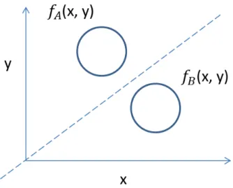
(12) Running head: Materials dimensionality and category learning. Figure 3. Mental representation structures transformed by different attentional weights on features. For. 政治大. example, there are total eight items defined by three dimensions, shape, size, and color. In this case, it is easier. 立. to differentiate two categories by color in structure of 3B than 3A.. ‧ 國. 學. The rule-based model, on the contrary, posits that to learn categories is to learn the rule. ‧. for defining categories. For instance, in Taiwan, a student’s studying performance can be. Nat. io. sit. y. regarded as two classes, pass and fail, depending on whether he/she gets a score larger than or. er. equal to 60. Although broadly speaking, rule can be of any format, this thesis focuses on the. al. n. v i n C h (GRT; Ashby &UGott, 1988) as the generic form of models of the general recognition theory engchi. the rule-based models. According to the GRT, each item is a percept in the psychological space and different categories correspond to different regions in this space separated by a decision boundary, namely a rule, as in Figure 4. Thus, if an item’s percept locates in the region corresponding to Category A, it will be classified to Category A. Accordingly, for the GRT, category learning is achieved when people form the decision bound(s) in the category learning task. 10.

(13) Running head: Materials dimensionality and category learning. Figure 4. Mental category representation divided by a decision bound. (Ashby & Gott, 1988). 治政 Although the rule-based and the similarity-based models 大 are quite different, they both 立 ‧ 國. 學. can predict human categorization behaviors very well (Maddox & Ashby, 1993, 1998; McKinley & Nosofsky, 1995, 1996). Thus, it is legitimate to posit that both types of. ‧. representations people would use. This idea was supported empirically by Rouder and. sit. y. Nat. io. n. al. er. Ratcliff (2004). These authors revealed that the exemplar-based model outperformed the. i n U. v. rule-based model when there were only few stimuli, whereas the rule-based model did when. Ch. engchi. there were a lot of exemplars. This finding is explained as when there are only few stimuli, people can remember all the exemplars in the category, hence, it is reasonable to compare a new stimulus to every exemplar in the original category before giving a categorical label, whereas people would tend to learn categorical bounds when too many exemplars to remember. Therefore, more and more models adopt the multiple representations view and these models are called multi-system model in this thesis. Besides, due to the rapidly progress in 11.

(14) Running head: Materials dimensionality and category learning. neural imaging techniques, some researchers suggests a multi-system theory not only in category learning (Ashby et al., 1998; Erikson & Kruschke, 1998; Nomura et al., 2007) but also other cognitive abilities or behaviors (Anderson & Lebiere, 1998; Sloman, 1996). Erickson and Kruschke (1998) presented a connectionist model called ATRIUM. This hybrid model consists of both the rule- and exemplar-based representation. The authors claim that participants learn categories by a mechanism incorporating these two kinds of modules. 政治大. for achieving the best performance and displays that ATRIUM can account for empirical data. 立. of categorization better than a single system model. COVIS (The Competition between verbal. ‧ 國. 學. and implicit systems) model is another famous multi-systems theory (Ashby et al, 1998).. ‧. COVIS model suggests that there are two independent subsystems of category learning: the. Nat. io. sit. y. rule-based subsystem (explicit system) and the procedural learning-based subsystem (implicit. er. system). The two subsystems would compete with each other and it has to be only one. al. n. v i n C hlearning. It wouldUnot be addressed here, as the issue subsystem to function during category engchi. of this present study is far from the main concern of the COVIS model. Before introducing the Sloutsky’s theory, which this study would address, two characteristics of category learning are discussed first.. Learning condition of categorization The studies mentioned above, from the research of Shepard et al. (1961) to the debate between similarity-based theory and rule-based theory (Maddox & Ashby, 1993, 1998; 12.

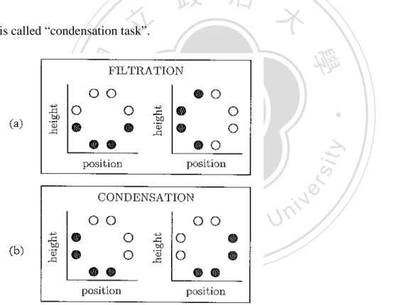
(15) Running head: Materials dimensionality and category learning. McKinley & Nosofsky, 1995, 1996; Nosofsky, Stanton, & Zaki, 2005; Stanton & Nosofsky, 2007), are mostly established by the evidences from supervised learning tasks. In a typical supervised learning task, participants would get a feedback or an instruction from each response. The feedback can be a visual message, like words of correct or wrong, or an auditory tone, like a high or low frequency beep. After receiving the feedbacks, participants can modify their learning strategies to approach the correct answers. Moreover, participants. 政治大. usually have little information at the beginning of task and learn the category rules through. 立. trial and error. Thus, it is reasonable that there are often many trials in a supervised learning. ‧ 國. 學. task. Besides supervised learning, unsupervised learning is another kind of conditions in the. ‧. experiments of category learning. In the unsupervised learning task, there is no any feedback. Nat. io. sit. y. from responses. Past studies showed that participants had different performances under. er. different conditions of learning (Ashby, Queller, & Berretty, 1999; Colreavy & Lewandowsky;. al. n. v i n C&hBohil, 2002). Actually, 2008; Love, 2002; Ashby, Maddox, e n g c h i U the unsupervised learning is much more similar to the ways we learn categories in our daily life.. Category structures As mentioned in the earlier paragraph, the category structure plays an important role on category learning (Shepard et al., 1961). Kruschke (1993) also found that “relevant dimensions” could influence participants’ performances. To explain further, assume there are two categories of the experiment materials (denoted as white and black circle in Figure 5), 13.

(16) Running head: Materials dimensionality and category learning. and each material could be represented by two dimensions of features, height and position, like Figure 5a and 5b. In the condition of Figure 5a, participants could differentiate materials in two categories by concentrating on only one dimension, either height (left) or position (right). This was named as “filtration task” because participants needed to filter out non-relevant dimensions and identify the relevant one for categorization. In the condition of Figure 5b, participants had to consider height and position dimensions simultaneously. Due to. 政治大. the fact that participants must condense multi-dimensions to one decision bound of category,. 立. this is called “condensation task”.. ‧. ‧ 國. 學. n. er. io. sit. y. Nat. al. Ch. engchi. i n U. v. Figure 5. Category structures of stimuli used in Kruschke’s study (1993).. The behavioral data showed that participants performed better on a filtration task than on a condensation task. Therefore, Kruschke (1993) concluded that the category learning task became harder when there were more relevant dimensions to be taken into account. The implications of Kruschke’s results are twofold. First, the category structure is more 14.

(17) Running head: Materials dimensionality and category learning. complicated in a condensation task than a filtration task. That is, participants need to consider both dimensions at the same time and it results in worse performances. Second, since Kruschke’s research was also based on the supervised learning, Kloos and Sloutsky (2008; see also in Sloutsky, 2010) argued that an immediate feedback could make an attentional shift more easily, which benefited the subjects’ performances by enhancing the cognitive processing of locating and focusing on a specific relevant dimension. It, however, became an. 政治大. obstacle when subjects needed to spread their attention on all dimensions at the same time,. 立. e.g., in a condensation task.. ‧ 國. 學. To sum up, not only the learning paradigm but also the category structure can influence. ‧. participants’ performances. Furthermore, some researches of developmental psychology. Nat. io. sit. y. suggest that children have different ways from adults to learn categorization, which may be. er. caused by the immaturity of brain area (Sowell, Thompson, Holmes, Batth, Jernigan, & Toga,. al. n. v i n 1999). Therefore, Sloutsky (2010) C develops systems theory of category learning, and h e na gdual chi U. tries to illustrate the relations among category structures, learning conditions, and categorical behaviors.. Sloutsky’s dual systems theory Sloutsky (2010) proposed a theory addressing the relationships among category representations, category structures, and learning conditions. This theory is one of the multi-system theories, as it assumes that the compression-based system and the 15.

(18) Running head: Materials dimensionality and category learning. selection-based system According to his theory, the manners people represent items are decided by category structures. In addition, these effects are detectable on the accuracy rates of various learning conditions. Like COVIS model (Ashby et al., 1998), Sloutsky also tries to connect the explicit and implicit memory systems to category learning mechanisms. He assumes that there are two subsystems, compression-based systems and selection-based systems, corresponding to the. 政治大. similarity-based system and the rule-based system respectively. During learning categories,. 立. which one of the two systems will function depends on category structure as well as learning. ‧ 國. 學. paradigm (e.g., supervised learning or unsupervised learning) (Sloutsky, 2010). In addition,. ‧. Sloutsky’s theory also has corresponding neural bases. The compression-based system is. Nat. io. sit. y. mainly related to the visual loop, which begins from the inferior temporal area through the. er. tail of caudate in the striatum (Segar & Cincotta, 2002), with many cortex neurons merged. al. n. v i n C h(Bar-Gad, Morris, U into a never bundle of caudate nucleus e n g c h i & Bergman, 2003). Since the visual. loop is in charge of recording visual information by reducing or compressing the visual input, the compression-based system is assumed to learn categories by recording the often appeared features (see Figure 6). Thus, the common features of highly similar exemplars, after being repeatedly presented, would be recorded by the compression-based system with little or even no attention. On the other hand, the selection-based system is assumed to be relevant to the cognitive loop, which goes through the prefrontal lobe and the head of caudate, and is 16.

(19) Running head: Materials dimensionality and category learning. activated during category learning process in a rule-based manner (Segar, 2008). The cognitive loop is related to the dorsolateral prefrontal cortex and the anterior cingulated cortex. Past studies found that this brain area is related to selective attention, working memory, and executive function (Cohen et al., 1997; Cohen, Botvinick, & Carter, 2000; D’Esposito, Postle, Ballard, & Lease, 1999). The manner of the selection-based system to learn categories is to select and focus on particular dimension(s) while ignoring the others.. 政治大. Therefore, it is suitable for learning the stimuli which can be classified by considering feature. 立. dimensions (Figure 7).. ‧ 國. 學. The coordination between the compression-based system and the selection-based system. ‧. follows “the winner takes all” rule, in that only one system would be executed in learning a. Nat. io. sit. y. category structure. The “default system” of these two systems is adjusted by the learning. er. condition and the category structure in adults. In contrast, past researches showed that. al. n. v i n Ch children do not develop the selection-based until four or five year-old (Kloos & e n gsystem chi U Sloutsky, 2008; Sloutsky, 2010). Therefore, the rule-based subsystem is apparently not the default learning system for children.. 17.

(20) Running head: Materials dimensionality and category learning. Figure 6. The learning progress of compression-based system (Sloutsky, 2010). This system records the most frequently occurring features.. 立. 政治大. ‧. ‧ 國. 學 sit. y. Nat. io. n. al. er. Figure 7. The learning progress of selection-based system (Sloutsky, 2010). This system is good at shift. attention to focus on specific dimension(s) and ignore others.. Ch. engchi. i n U. v. Statistical density Sloutsky’s dual systems theory posits that people use different learning systems depending on “what materials look like”, i.e., the category structure (Kloos & Sloustky, 2008; Sloutsky, 2010). That is, whether people would use the selection-based system or the compression-based system to learn the category task can be predicted by considering the composition of materials, specifically the category structure. In order to make different 18.

(21) Running head: Materials dimensionality and category learning. category structures comparable, Kloos and Sloutsky (2008) proposed an index named the statistical density. The calculation of statistical density is based on “entropy” in the information theory (Shannon, 1948). The entropy in Sloutsky’s dual system theory represents the extent of randomness, while the statistical density represents the regularity of stimuli. The relation between entropy and statistical density can be described as D=1−. Hwithin. Hbetween. ,. Equation 2. 政治大. where D denotes the density and H denotes the entropy. When Hbetween remains constant,. 立. the larger the within-category entropy is, the lower the density becomes. On the other hand, if. ‧ 國. 學. ‧. Hwithin stays constant, the larger the between-category entropy is, the higher the density. becomes. According to Sloutsky, the compression-based system would be used when D is. Nat. io. sit. y. large, whereas the selection-based system would be activated when D is small. The. er. within-category entropy, Hwithin , is the variability of items within the target category, while. al. n. v i n C h , is acquired by U Hbetween e n g c h i considering the variability between. the between-category entropy,. the target category and the contrasting category. The within-category entropy is the sum of the dimensional and relational entropy within a category and the between-category entropy is the sum of the dimensional and relational entropy between categories, which are respectively computed as dim rel Hwithin = Hwithin + Hwithin and dim rel Hbetween = Hbetween + Hbetween .. Equation 3-1 Equation 3-2 19.

(22) Running head: Materials dimensionality and category learning. In addition, Hwithin would not be bigger than Hbetween because the within-category. variability is also considered in the calculation of Hbetween . Thus, the density is a number. between 0 and 1.. The dimensional entropy within category and between categories are computed as dim Hwithin = − ∑M i=1 wi [∑j=0,1 within(pj log 2 pj )] and. Equation 4-1. dim Hbetween = − ∑M i=1 wi [∑j=0,1 between(pj log 2 pj )]. Equation 4-2. 政治大. where, for the within-category case, pj is the percentage of feature j on one dimension within. 立. a category, whereas, for the between-category case, pj is the percentage of feature j on one. ‧ 國. 學. dimension across categories. For instance, if the stimuli of the target category are all black. ‧. and the contrasting category are all white, then pj=1 = 1 (j=1 for black and j=0 for white) on. Nat. y. sit. io. color dimension in the within-category case, whereas pj=1 = 0.5 in the between-category. n. al. er. case. The dimensional entropy is the sum of the material variability on m dimensions, each of. Ch. engchi. which is weighted by an attention weight, w.. i n U. v. Different from the dimensional entropy, the relational entropy concerns the extent of variability between every pair of dimensions, which is computed for the within-category case as well as the between-category cases as rel = − ∑O Hwithin i=1 wk [∑m=0,1 within(pmn log 2 pmn )] and n=0,1. rel Hbetween = − ∑O i=1 wk [∑m=0,1 between(pmn log 2 pmn )] with. O = C2M =. M! . (M−2)!∗2!. n=0,1. Equation 5-1 Equation 5-2 Equation 6. 20.

(23) Running head: Materials dimensionality and category learning. For M dimensions, there would be O = C2M pairs. As the dimensions are dyadic, there. would be four combinations of the feature values for each pair. Accordingly, pmn is the. probability of one of the combinations between “feature m” and “feature n”. The variability information of different pair is differently weighted by the attention weight, wk . For instance, if the target category members are all black squares while the contrasting category members. are all white circles, the within-category variability of the color-shape pair for all four value. 政治大. combinations is 1, 0, 0, and 0 in the order of black-square, black-circle, white-square, and. 立. black-square, black-circle, white-square, and white-circle.. 學. ‧ 國. white-circle. However, the between-category variability is 0.5, 0, 0.5, and 0 in the order of. ‧. Kloos and Sloutsky (2008) conducted a series of experiments and reviewed past. Nat. io. sit. y. literature to estimate the salience of varying dimensions. They led into a conclusion that the. al. er. attentional weight of a particular dimension (wi ) was twice as large the dyadic relation. n. v i n Ci . hIn order to compute wk = 2 w e n g c h i U density in. between dimensions wk ,. 1. an easier way, the. dimensional attention weight, wi , is set as 1 and the relational weight, wk , is set as 0.5 in the current study.. Statistical density is a convenient index to represent category structures. To illustrate this index in detail, two examples showing the calculation of density are included in the Appendix.. 21.

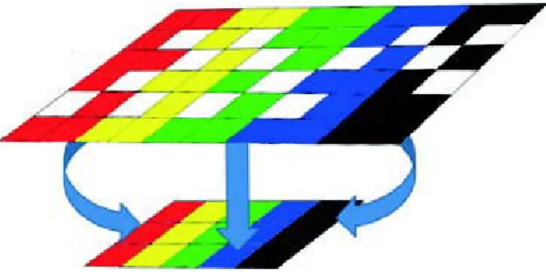
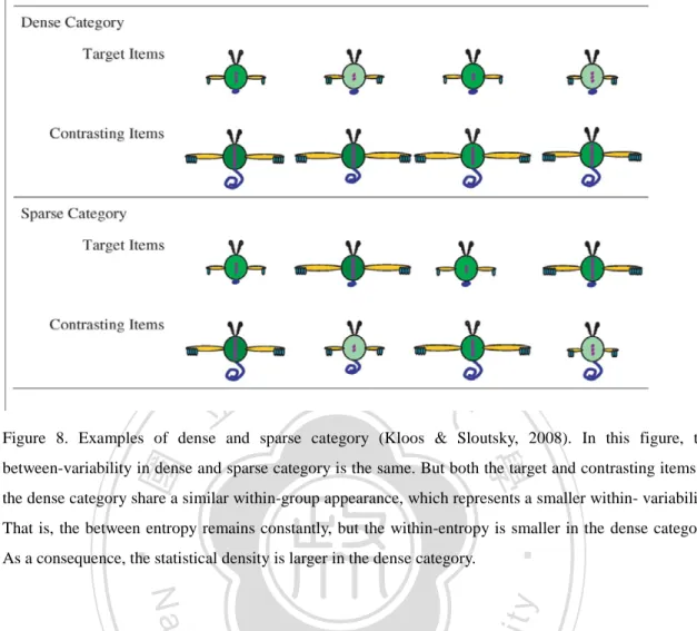
(24) Running head: Materials dimensionality and category learning. Incongruent evidence with Sloustky’s dual systems theory The main idea of Sloutsky’s dual systems theory is to describe the relationship between category structures (in terms of density), conditions of learning, and category representations (Sloutsky, 2010). Because of the characteristics of the compression-based system and the selection-based system, Sloutsky predicts an interaction effect between learning conditions and category structures. Namely, the selection-based system would function during learning a low density category and improve the performance on the supervised learning condition,. 政治大 whereas the compression-based system would function during learning a high density 立. ‧ 國. 學. category and improve the performance on the unsupervised learning condition. Kloos and Sloustky (2008) found that when learning categorization in the condition of dense category. ‧. sit. y. Nat. (high density, displayed in the upper part of Figure 8), participants performed better under the. n. al. er. io. unsupervised learning condition than under the supervised learning condition. On the contrary,. i n U. v. participants performed better under the supervised learning conditions than under the. Ch. engchi. supervised learning in the condition of sparse category, when learning the low-density category structures (shown in the lower part of Figure 8). From now on, the high-density category structure is called the dense category and the low-density category structure is called the sparse category.. 22.

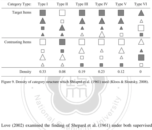
(25) Running head: Materials dimensionality and category learning. 立. 政治大. Figure 8. Examples of dense and sparse category (Kloos & Sloutsky, 2008). In this figure, the. ‧ 國. 學. between-variability in dense and sparse category is the same. But both the target and contrasting items in the dense category share a similar within-group appearance, which represents a smaller within- variability.. As a consequence, the statistical density is larger in the dense category.. Nat. io. sit. y. ‧. That is, the between entropy remains constantly, but the within-entropy is smaller in the dense category.. er. However, Sloutsky’s dual systems theory has difficulty accounting for the learning. al. n. v i n C h reported by Shepard difficulty gradient over category structure e n g c h i U et al. (1961). Figure 9 shows. those category structures as well as their statistical densities. Shepard and his colleagues (1961) conducted their experiments in the condition of supervised learning. According to Sloutsky’s (2010) opinion, the supervised learning condition would trigger the selection-based subsystem, which is suitable to learn the sparse categories rather than the dense ones. Therefore, type VI category structure (density = 0; sparse category) should be learned better in the supervised learning condition, while type I (density = 0.33; dense 23.

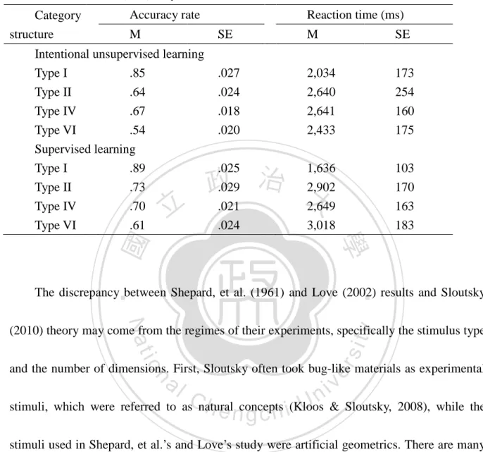
(26) Running head: Materials dimensionality and category learning. category) should be learned worse. However, Shepard et al. (1961), conversely, found that Type I was learned better than Type VI in the supervised learning condition.. 立. 政治大. ‧ 國. 學 ‧. Figure 9. Density of category structure which Sheaprd et al. (1961) used (Kloos & Sloutsky, 2008).. er. io. sit. y. Nat. al. n. v i n C h of Shepard et al.U(1961) under both supervised and Love (2002) examined the finding engchi unsupervised learning conditions and found that participants performed better on Type I and worse on Type VI in no matter which learning condition, see in Table 1. This result challenges the Sloutsky’s dual systems theory which predicts an interaction effect between the density and the learning condition.. 24.

(27) Running head: Materials dimensionality and category learning. Table 1. Results of Love’s (2002) study. Category structure. Accuracy rate M. Intentional unsupervised learning Type I .85 Type II .64 Type IV .67 Type VI .54 Supervised learning Type I .89 Type II .73 .70 Type IV Type VI .61. 立. Reaction time (ms) SE. M. SE. .027 .024 .018 .020. 2,034 2,640 2,641 2,433. 173 254 160 175. 1,636 治政 2,902 大 2,649. 103 170 163 183. .025 .029 .021 .024. 3,018. ‧. ‧ 國. 學. The discrepancy between Shepard, et al. (1961) and Love (2002) results and Sloutsky. y. Nat. er. io. sit. (2010) theory may come from the regimes of their experiments, specifically the stimulus type and the number of dimensions. First, Sloutsky often took bug-like materials as experimental. al. n. v i n C h concepts (Kloos stimuli, which were referred to as natural e n g c h i U & Sloutsky, 2008), while the stimuli used in Shepard, et al.’s and Love’s study were artificial geometrics. There are many. studies showing the performance of participants could be influenced by the kinds of stimuli used (Love, 2003; Markman & Makin, 1998; Markman & Ross, 2003). Second, the stimuli in Kloos and Sloutsky’s (2008) experiment had six, eight or ten dimensions (e.g. length of wings, color of body, number of fingers, etc.; as shown in Figure 8). In contrast, the materials had only three dimensions in Shepard’s study, and four in Love’s, which were substantially 25.

(28) Running head: Materials dimensionality and category learning. simpler in the respect of visual perception. The past research revealed that the learning strategy of participants could be influenced by the dimensionality of materials (Minda & Smith, 2001). In addition, Livingston, Andrews, and Harnad (1998) found that the dimensions of stimuli could mediate different effects in category perception. Namely, the distances between each member of the same category become closer after category training, the within-compression effects, were only observed when stimuli varied in two dimensions,. 政治大. but did not appear in one dimension. This result indicates that people perceive the category. 立. concepts differently when the number of stimulus dimensions is in different level.. ‧ 國. 學. As a consequence, the aim of this study is to illustrate the reasons making inconsistent. ‧. results among Sloutsky’s theory (2010; see also in Kloos & Sloutsky, 2008) and the past. Nat. io. sit. y. researches (Shepard et al, 1961; Love, 2002). Through the literature reviews and the direct. er. comparison of the experimental settings of these researches, this study focuses on two. al. n. v i n C hof stimuli and theUkinds of stimuli used. According to possible factors, the overall dimensions engchi Sloutsky’s theory, human learn categories. by either selection-based system or. compression-based system which depends on the statistical density, i.e., category structure. Thus, an interaction between category structure and representation is predicted. Besides, the characteristics of supervised and unsupervised learning condition make different effects during the learning of different subsystems, which indicates that an interaction between learning condition and category structure in terms of learning performance is also predicted. 26.

(29) Running head: Materials dimensionality and category learning. However, if the predicted interactions are not displayed under the manipulations of different stimuli used or overall dimensions of stimuli, which means that the Sloutsky’s dual systems theory needs to be modified under certain circumstances.. 立. 政治大. ‧. ‧ 國. 學. n. er. io. sit. y. Nat. al. Ch. engchi. 27. i n U. v.

(30) Running head: Materials dimensionality and category learning. Methods Experiment 1 According to Sloutsky’s theory, the unsupervised learning condition would trigger the compression-based system, which suits the dense category structure, whereas the supervised learning condition would trigger the selection-based system, which suits the sparse category structure. Also, the dimensionality of material has nothing to do with the correspondence between category structure and learning condition. In order to examine this idea, two groups. 政治大 of participants were recruited, each for learning one type of category structure (dense or 立. ‧ 國. 學. sparse). Each participant was asked to learn the assigned category structure with two types of dimensionality (eight vs. four dimensions) in two learning conditions (supervised learning vs.. ‧. sit. y. Nat. unsupervised learning). If there is no difference on the interaction effect (category structure x. n. al. er. io. learning condition) with either material dimensionality, Sloutsky’s theory is supported. Same. i n U. v. as in the first and second experiment of Kloos and Sloutsky (2008), the artificial bug-like. Ch. engchi. materials were used in this experiment (see Figure 10 and Figure 11).. Apparatus The experiment was conducted in a quiet testing booth and the procedure and data collection were done by a Matlab program with the aid of Psychtoolbox version 2.5.4 (Brainard, 1997; Pelli, 1997) on an IBM compatible PC.. 28.

(31) Running head: Materials dimensionality and category learning. Participants Ninety-eight undergraduate and graduate college students took part in the task voluntarily and were reimbursed with a small amount of money for their traffic expense. Participants were assigned equally to the conditions of dense or sparse categories. The age of these participants ranged from 18 to mid 30s. All participants’ visions were reported normal or corrected to normal.. 立. Stimulus. 政治大. ‧ 國. 學. In the condition of low dimensionality, the stimuli were composed of four binary dimensions, the shading of antennas (dark or light colour), the number of fingers (many or. ‧. y. sit. n. al. er. io. (Figure 10).. Nat. few), the length of wings (long or short), and the shading of the body (dark or light colour). Ch. engchi. i n U. v. Figure 10. Examples of low dimensionality (4 dimensions) stimuli used in Experiment 1. The left figure has dark antennas, many fingers, dark body color, and short wings. The right one has light antennas, few fingers, light body, and long wings.. 29.

(32) Running head: Materials dimensionality and category learning. In the condition of high dimensionality, the stimuli varied along eight dimensions. In addition to the four dimensions used in the low dimensionality condition, the other four dimensions were: the length of fingers (long or short), the length of the tail (long or short), the number of buttons (many or few), and the shading of buttons (dark or light) (Figure 11). These eight dimensions were just same as Kloos and Sloutsky (2008) used in their fourth experiment.. 立. 政治大. ‧. ‧ 國. 學 sit. y. Nat. al. er. io. Figure 11. Examples of high dimensionality (8 dimensions) stimuli used in Experiment 1. The right figure has. v. n. dark antennas, many and long fingers, dark body color, long tail, many and dark color buttons, and long wings.. Ch. i n U. The left one has light antennas, few and short fingers, light body, few and light color buttons, and long wings.. engchi. Stimuli were generated as either in the statistically dense category or in the statistically sparse category. The statistical density of the dense category was 0.50 in the high dimensionality condition, and the sparse category was 0.13. In the condition of low dimensionality, the density of the dense category was 0.36, while the sparse category was 0.10. The dense category represented a category structure which had high similarity of target items, but looked quite different between target category and contrasting category (see Figure 30.

(33) Running head: Materials dimensionality and category learning. 8). Because the items could not be categorized by only few features, the better way to classify would be consider the overall appearance of stimuli. In contrast, in the sparse category structure, the members in the target category were less similar to each other. Thus, categorization became easier with only few specific features. These specific features were named as “arbitrary rules” in the sparse category condition, because the participants could decide to which category a stimulus belonged by these features only. Table 2 and 3 showed. 政治大. the category structure used in this experiment.. 立. The target items of the dense category in the low dimensionality condition (i.e., four. ‧ 國. 學. dimensions) were set to have short wings, light color of antennas, light color of body, and few. ‧. fingers, while the contrasting items had long wings, dark color of antennas, dark color of. Nat. io. sit. y. body, and many fingers. On the other hand, in the high dimensionality condition, the target. n. al. er. items of the dense category had short wings, light colour of antennas, light color of body, few. Ch. engchi. fingers, short fingers, short tails, few buttons, and. iv n light U colour. of buttons, while the. contrasting items had long wings, dark color of antennas, dark color of body, many fingers, long fingers, long tails, many buttons, and dark colour of buttons. In addition, the four features, length of wings, shading of antennas, shading of body, and number of fingers were equally likely to be chosen as the arbitrary rule in sparse category, in order to prevent the feature specific effect on learning the rule.. 31.

(34) Running head: Materials dimensionality and category learning. Table 2. Category Structure of Stimuli Used in 4 dimensions in Experiment 1. Dense category. Dimension length of wings Shading of antennas Shading of body Number of fingers. Sparse category. Target item Contrast item. Target item. Contrast item. 0 0 0 0. 0 … … …. 1 … … …. 1 1 1 1. Note. The numbers 0 and 1 refer to the values of each dimension (e.g., 0 is light color, while 1 is dark color). The “…” represents the varied randomly features.. 政治大立Dense category. Table 3. Category Structure of Stimuli Used in 8 dimensions in Experiment 1. y. 0 … … … … … … …. er. io. al. 1 1 1 1 1 1 1 1. ‧. 0 0 0 0 0 0 0 0. Nat. Length of wings Shading of antennas Length of tails Length of fingers Number of buttons Shading of buttons Shading of body Number of fingers. Target item. 學. ‧ 國. Target item Contrast item. Sparse category. sit. Dimension. Contrast item 1 … … … … … … …. n. v i n Note. The numbers 0 and 1 refer to the values C hof each dimension (e.g.,U0 is light color, while 1 is dark color). The “…” engchi represents the varied randomly features.. For the reason of testing the vigilance of participants, eight new items were added into the testing phase, which consisted of new features such as that they had a multi-colour body in a hexagonal shape, no finger, and no tail (Figure 12). Because these pictures had dissimilar appearances and different values of features, it was expected that the participants could reject those items accurately. 32.

(35) Running head: Materials dimensionality and category learning. Figure 12. Examples of vigilance pictures used in Experiment 1. These pictures are supposed to be rejected in the testing phase.. 立. Procedure. 政治大. ‧ 國. 學. Each participant took in turn four sessions to learn stimuli of two complexities using two. ‧. types of learning. The sequence of the four sessions was generated from a Latin square design.. Nat. sit er. io. testing phase.. y. In each session, there were four blocks, each of which contained a training phase with and a. al. n. v i n C hwere asked to learnUthe target category called “Ziblet” In the training phase, participants engchi in a self-pace manner. The participants were given the information about the target item in verbal sentences (supervised learning) or in graphical figures (unsupervised learning). In the supervised learning condition, the verbal rules were listed on screen directly, while in the unsupervised learning condition, sixteen pictures of target items were displayed in a random sequence. Participants were told to remember the verbal rules and the pictures as possible as they could in the training phase. In addition, there was no any feedback in this section.. 33.

(36) Running head: Materials dimensionality and category learning. In order to make sure that the participants understood the name of every feature, the computer program would firstly show the feature and its corresponding name simultaneously in the beginning of every training phase. For instance, the picture of fingers and the name “finger” were both showed together on the screen. In the testing phase, the participants were asked to answer whether or not the present pictures belonged to the target category. Sixteen pictures belonging to target category and. 政治大. sixteen pictures belonging to contrasting category were used in the testing phase. An. 立. additional eight vigilance pictures were added to examine whether the participants. ‧ 國. 學. concentrated properly in the experiment. If more than three vigilance pictures were not. ‧. rejected correctly in a block, the data of the participant would be excluded from further. Nat. n. al. er. io. sit. y. analyses. Therefore, a total of 40 pictures were used in the testing phase.. Results. Ch. engchi. i n U. v. Twenty subjects were excluded (10 out of 49 in the sparse category condition, and 10 out of 49 in the dense category condition) from data analyses, due to their failures to reject the pictures of vigilance testing (data was excluded if there was any condition that participant did not correctly reject at least 5 of 8 vigilance pictures). The accuracy rates of 32 items in the testing phases (without the eight vigilance pictures) of each participant were computed to examine the learning of the target category. A 2 (Density) × 2 (Dimensionality) × 2 34.

(37) Running head: Materials dimensionality and category learning. (Learning Condition) mixed-design ANOVA revealed that the 3-way interaction was not significant (F(1, 76) = 0.44, MSe = 0.09, p = .51, η2 = 0.01). The 2-way interaction was significant only between Learning condition × Density (F(1, 76) = 6.61, MSe = 0.09, p < .05, η2 =0.08), but not significant either between Learning condition × Dimensionality (F(1, 76) = 1.57, MSe = 0.09, p = .22, η2 = 0.02) or Density × Dimensionality (F(1, 76) = 0.01, MSe = 0.08, p = .91, η2 = 0.00). The main effects of Density (F(1, 76) = 56.91, MSe =. 政治大. 0.18, p < .01, η2 = 0.43) and Dimensionality (F(1, 76) = 5.08, MSe = 0.07, p < .05, η2 =0.06). 立. were significant, but Learning condition (F(1, 76) = 0.01, MSe = 0.09, p = .92, η2 = 0.00) was. ‧ 國. 學. not. Slousky’s theory predicts an interaction between Density and Learning condition with no. ‧. matter how complex the stimulus is. However, as discussed about Love’s (2002) results in the. Nat. io. sit. y. previous section, the interaction effect between Density and Learning condition may. er. disappear when the dimensionality of materials is low. Visual inspection on Figure 13 implies. al. n. v i n C hLearning conditionUonly when the Density and engchi. an interaction between. material is more. complex (i.e., 8 dimensions). This observation was supported by the analysis for the interaction effects, that the interaction effect between Density and Learning condition was significant for high dimensionality materials (F(1, 76) = 4.97, p < .05, MSe = 0.2, η2 =0.06), but not significant for low dimensionality materials (F(1, 76) = 2.00, MSe = 0.17, p = .16, η2 =0.02).. 35.

(38) Running head: Materials dimensionality and category learning. Therefore, the result of this experiment reveals that dimensionality does influence category learning, which also means Sloutsky’s theory should be modified by taking into consideration the dimensionality of materials.. 8-dimensions. 4-dimensions. 1. 1. 0.95. 0.95. 0.9. 0.9. 0.85. 0.85. 政治大 0.8. 0.75. Hits. Hits. 0.8. 立. 0.7. Dense. 0.6 0.55 0.5. Sparse. Dense. Category Structure. sit. y. Nat. Category Structure. ‧. 0.55. 0.7 0.65. ‧ 國. 0.6. 0.75. 學. 0.65. 0.5. Unsupervised learning Supervised learning. n. al. er. io. Figure 13. Mean accuracy scores by category type and learning condition in Experiment 1.. Ch. engchi. 36. i n U. v. Sparse.

(39) Running head: Materials dimensionality and category learning. Experiment 2 The previous experiment reveals that the dimensionality of materials in terms of the number of dimensions would moderate the learning performance. In addition to the dimensionality of materials, the type of stimulus may also result in the different findings of Love (2002) and Shepard et al. (1961) from Sloutsky’s. In Kloos and Sloutsky’s study (2008), they mainly used natural-like stimuli which were composed of natural-like features such as wings, tails, antennas, etc. However, the stimuli used in the studies of Shepard et al. (1961). 政治大 and Love (2002) were artificial geometrics, such as a dark large circle, etc. Therefore, 立. ‧ 國. 學. Experiment 2 was designed to examine the effect by using artificial geometrics. For a parallel comparison with Experiment 1, Experiment 2 adopted the experimental design of Experiment. ‧. sit. y. Nat. 1, manipulating Density (between-subject variable), Dimensionality (within-subject variable),. n. al. er. io. and Learning condition (within-subject variable), but using the artificial geometrics as stimuli.. Ch. engchi. i n U. v. Participants Eighty-five college students were recruited with traffic reimbursement of one-hundred NT dollars per hour for their expense of time and money. For the density category condition, there were thirty-six participants and forty-nine for the sparse category condition. The age of these participants ranged from 18 to mid 30s. All participants reported that his/her vision was normal or corrected to normal. 37.

(40) Running head: Materials dimensionality and category learning. Stimulus The dense and sparse categories were defined by the same way used in Experiment 1. Also, same as in Experiment 1, the extent of material dimensionality was defined by the number of features (4 vs. 8). The low-dimensionality material consisted of four binary features: the shape of figure (square vs. rectangle), the color of figure (blue vs. purple), the color of frame (red vs. yellow), and whether there was a dot in the circle (Figure 14). The high-dimensionality material consisted of the four features of the low-dimensionality material. 政治大 and the other four features: the number of frame lines (1 vs. 2), the size of figure (big vs. 立 ‧. ‧ 國. (Figure 15).. 學. small), whether the figure was open or closure, and whether there was a diagonal line or not. n. er. io. sit. y. Nat. al. Ch. engchi. i n U. v. Figure 14. Examples of stimuli in low dimensionality used in Experiment 2. The left geometric is a rectangle with red frame line, purple body, and a dot in the middle, while the right one is a square with yellow frame line, blue body, and there is no dot in it.. The target items of the dense category in low dimensionality were purple squares with red frame line, while the contrasting items were blue rectangles with yellow frame line and a dot in the middle. The target items of the dense category in high dimensionality were small, 38.

(41) Running head: Materials dimensionality and category learning. 立. 政治大. 學. ‧ 國. Figure 15. Examples of stimuli in high dimensionality used in Experiment 2. The left geometric is a big, open square with one yellow frame line, and there is no dot or diagonal line. The right figure is a small, closure rectangle with two red frame lines, a dot in the middle, and a diagonal line.. ‧. purple, and closure squares with one frame line in red color, while the contrasting items were. Nat. a diagonal line inside the figure (Table 4 and Table 5).. n. al. Ch. engchi. er. io. sit. y. big, blue, and open rectangles with two frame lines in yellow color, and there were a dot and. i n U. v. Figure 16. Examples of vigilance pictures used in Experiment 2. These pictures are supposed to be rejected.. 39.

(42) Running head: Materials dimensionality and category learning Table 4. Category Structure of Stimuli Used in 4 dimensions in Experiment 2. Dense category. Dimension. Sparse category. Target item. Contrast item. Target item. Contrast item. 0 0 0 0. 1 1 1 1. 0 … … …. 1 … … …. Shape of figure Color of frame line Color of figure A dot in the middle. Note. The numbers 0 and 1 refer to the values of each dimension. The “…” represents the varied randomly features.. Table 5. Category Structure of Stimuli Used in 8 dimensions in Experiment 2. Dense category Target item. 立. Contrast item 1 …. 1. …. …. 0 0 0 0 0. 1 1 1 1 1. … … … … …. … … … … …. y. Nat. 0. ‧. ‧ 國. 0 0. Contrast item Target item 政1 治大 0 1 …. 學. Shape of figure Color of frame line Number of frame line Color of figure Size of figure Open or Closure A dot in the middle Diagonal line. Sparse category. io. sit. Dimension. al. n. features.. er. Note. The numbers 0 and 1 refer to the values of each dimension. The “…” represents the varied randomly. Ch. engchi. i n U. v. Same as in Experiment 1, the figure shape, the figure color, the color of frame line, and the presence of dot, had a same probability to make up the arbitrary rule in the sparse category. Also, there were eight vigilance pictures added in the testing phase (Figure 16). The statistical density of the dense category was as same as Experiment 1, 0.50 in the high dimensionality condition, and the sparse category was 0.13. In the condition of low dimensionality, the density of the dense category was 0.36, while the sparse category was 0.10.. 40.

(43) Running head: Materials dimensionality and category learning. Procedure Except for the stimuli replaced by artificial geometrics, the experimental procedure was exactly as same as Experiment 1. Participants were asked to learn the “Ziblet” category in the training phase, and they needed to judge whether the each figure appearing in the testing phase belonged to the “Ziblet” category or not.. Results. 政治大 Thirteen subjects were excluded from data analyses, due to their failure to reject the 立. ‧ 國. 學. pictures for vigilance testing. A 2 (Density) × 2 (Dimensionality) × 2 (Learning condition) mixed-design ANOVA revealed that the 3-way interaction is not significant (F(1, 70) = 3.02,. ‧. sit. y. Nat. MSe = 0.03, p = .09, η2 = 0.04). The 2-way interaction was found significant between. n. al. er. io. Learning condition and Density (F(1, 70) = 14.42, MSe = 0.04, p < .01, η2 =0.17), but not. i n U. v. significant either between Learning condition × Dimensionality (F(1, 70) = 0.00, MSe =. Ch. engchi. 0.03, p = .97, η = 0.00), or Denisty × Dimensionality (F(1, 70) = 0.16, MSe = 0.04, p = .69, 2. η2 = 0.02). Significant main effects of Density (F(1, 70) = 29.49, MSe = 0.06, p < .01, η2 = 0.30), Learning condition (F(1, 70) = 5.12, MSe = 0.04, p < .05, η2 = 0.07) and Dimensionality (F(1, 70) = 5.52, MSe = 0.04, p < .05, η2 =0.07) were found.. 41.

(44) Running head: Materials dimensionality and category learning. The interaction effect of Density × Learning condition was significant when the. material dimensionality was high (F(1, 70) = 19.16, MSe = 0.06, p < .01, η2 =0.22), but not significant when the material dimensionality was low (F(1, 70) = 2.66, MSe = 0.08, p = .11) (See Figure 17).. 8-dimensions. 4-dimensions. 1. 1. 0.95. 0.95. 政治大. 0.9. 0.9. 0.85. 0.85. 立. Hits. ‧ 國. 0.65. Dense. 0.6. Nat. 0.55. 0.65. ‧. 0.6. 0.7. 0.55 0.5. Sparse. io. Dense. Sparse. Category Structure. n. al. er. Category Structure. y. 0.7. 0.75. sit. 0.75. 0.8. 學. Hits. 0.8. 0.5. Unsupervised learning Supervised learning. Ch. i n U. v. Figure 17. Mean accuracy scores by category type and learning condition in Experiment 2.. engchi. Same as found in Experiment 1, the interaction between Density and Learning condition appeared only when the material dimensionality was high. This result strengthens the challenge to Sloutsky’s theory with a different type of stimuli. Also, the categories were ill defined in Kloos and Sloutsky (2008) as “Most Ziblets have long wings and dark antennas”, whereas the categories in this experiment as well as in the studies of Shepard et al. (1961) and Love (2002) were well defined, as there was no exception to the definition of categories. 42.

(45) Running head: Materials dimensionality and category learning. Therefore, this result shows that whether the categories were ill defined or well defined is not the cause for the discrepancy in the past research results. Considering the results of both Experiment 1 and Experiment 2, the dimensionality of material plays a crucial rule in category learning, which is not considered in Sloutsky’s theory.. 立. 政治大. ‧. ‧ 國. 學. n. er. io. sit. y. Nat. al. Ch. engchi. 43. i n U. v.

(46) Running head: Materials dimensionality and category learning. Experiment 3 Both Experiment 1 and Experiment 2 consistently indicate the dimensionality of materials can influence the category learning performance that is not predicted by Sloutsky’s theory. That is, the expected interaction effect between the density of category structure and the learning manner only occurs for high dimensionality materials. Since the interaction effect is assumed to result from that the dense and sparse category structures respectively. 政治大. triggers the compression-based system and the selection-based system, it is worth examining. 立. the learning system on which the participants rely to learn different category structures,. ‧ 國. 學. specifically when the stimulus materials are of different complexities.. ‧. Following the fourth experiment of Kloos and Sloutsky (2008), this experiment added. y. Nat. er. io. sit. diagnostic items in the test phase in order to examine which learning system was activated. The diagnostic items could be separated to two classes. One looked dissimilar to the target. n. al. Ch. engchi. i n U. v. item but shared with the target item the arbitrary rule feature (i.e., the defining feature of the rule). The other looked similar to the target item but did not have the rule feature of the target item. If the dissimilar-appearance diagnostic item was classified to the target category, then it was indicated that the selection-based system was activated and. On the other hand, when the compression-based system was activated, participants should classify the similar-appearance diagnostic items to the target category.. 44.

(47) Running head: Materials dimensionality and category learning. Participants Ninety-one participants were recruited in this experiment with traffic reimbursement of one-hundred NT dollars per hour for their expense of time and money. The participants were randomly assigned to one of four conditions (learning the dense vs. sparse category under low vs. high dimensionality). The age of these participants ranged from 18 to mid 30s. All participants reported that his/her vision was normal or corrected to normal.. Stimulus. 政治大 The stimuli in this experiment were the same as in Experiment 1, except that two types 立. ‧ 國. 學. of the diagnostic items were added. Each stimulus was composed of two types of features: the rule feature and the appearance feature. The rule feature was the one that could predict the. ‧. sit. y. Nat. target category 100% correct, whereas the appearance feature could not. The diagnostic item. n. al. er. io. ACRT looked dissimilar to the target item (i.e., the appearance features had values of the. i n U. v. contrasting category) but had the same value of the rule feature as the target item did. On the. Ch. engchi. contrary, the diagnostic item ATRC looked similar to the target item (i.e., the appearance features had values of the target category) but had a different value of the rule feature as the target item did. The same naming principle could be applied to the other two types of items (ACRC and ATRT). For the low dimensionality materials, the feature of the number of fingers was set as the arbitrary rule. For the high dimensionality materials, the arbitrary rule was defined by the relation between the length of fingers and the shading of body. Table 6 and Table 7 all four types of items in the low and high dimensionality condition respectively. 45.

(48) Running head: Materials dimensionality and category learning Table 6. Examples of Stimuli Used in the Low Dimensionality Condition of Experiment 3 Presented in Abstract Notation. Feature Appearance Length of wings Shading of antennas Shading of body Rule Number of fingers. AT R T. AT R C. AC R T. AC R C. 0 1 0. 0 1 0. 1 0 1. 1 0 1. 0. 1. 0. 1. Note. The numbers 0 and 1 refer to the values of each dimension.. The statistical density of the dense category was 0.38 in the high dimensionality. 治政大 of low dimensionality, the condition, and the sparse category was 0.01. In the condition 立 ‧. ‧ 國. 學. density of the dense category was 0.36, while the sparse category was 0.1.. al. Ex 1. Ch. Length of tail Length of wings. 0 0. 0 0. Shading of antennas Number of fingers Shading of buttons. 1 0 0. 1 0 0. 1 0 0. Number of buttons Rule. 1. 1. Length of fingers Shading of body. 1 0. 0 1. Ex 2. 0. 0. Ex1. AC R T. sit. Ex 2. AT R C. Ex 2. er. Ex 1. n. Appearance. AT R T. io. Feature. Nat. notation.. y. Table 7. Examples of stimuli used in the high dimensionality condition of Experiment 1 presented in abstract. i n 1 U. v. Ex 1. AC R C. Ex 2. 1. 1 1. 1 1. 1 1. 1 0 0. 0 1 1. 0 1 1. 0 1 1. 0 1 1. 1. 1. 0. 0. 0. 0. 1 1. 0 0. 1 0. 0 1. 1 1. 0 0. e 0n g c h0 i. Note. There are two examples of each type of items (Ex1 and Ex2). The number 0 and 1 refer to the values of each dimension.. 46.

(49) Running head: Materials dimensionality and category learning. Procedure In the beginning of the training phase, the experimenter firstly introduced all the features (the number of features depend on the experimental condition) to the participants. And then both verbal and graphic information of the target items were provided on the computer screen. The verbal rules were showed first, and then the graphs of the target stimuli were presented in a random sequence (eight pictures were also chosen randomly). Participants were told that they would receive the information of target category only in the training phase and. 政治大 instructed to learn both the verbal and graphical messages in a self-pace manner. After the 立. ‧ 國. 學. training phase, the participants were given a recognition task incidentally. In this task, the participants were asked to recognize whether the present stimulus was seen in the training. ‧. sit. y. Nat. phase. Sixteen stimuli including eight ATRT pictures (which were showed in the training. n. al. er. io. phase) and eight ACRC pictures were presented in a random sequence. The data of the. i n U. v. participant who could answer correctly at least eleven out of sixteen trials in the recognition. Ch. engchi. task were included in further data analyses.. In the testing phase, the participants were asked to judge for every single stimulus whether or not it belonged to the target category. The stimuli used in the testing phase were eight ATRC pictures and eight ACRT pictures presented in a random sequence. Results Twelve participants were excluded from data analyses due to failure to meet the criterion of the recognition task. The proportion of the diagnostic items classified to the target category 47.

(50) Running head: Materials dimensionality and category learning. is shown in Figure 18. Apparently, the participants rely on the selection-based system to make classification for the low dimensionality materials (the right panel), regardless of the density of category structure, as a large amount of the ACRT items are classified to the target category and so are a small amount of the ATRC items. However, for the high dimensionality materials, only when learning the sparse category structure, there are more ACRT items than ATRC ones classified to the target category (the left panel).. 立. 政治大. ‧. ‧ 國. 學. n. er. io. sit. y. Nat. al. Ch. engchi. i n U. v. Figure 18. Mean accuracy scores by category type and learning condition in Experiment 3.. A 2 (Dimensionality) × 2 (Density) × 2 (Foil type: ATRC and ACRT) mixed-design. ANOVA was conducted. The 3-way interaction was not significant (F(1, 75) = 1.75, MSe = 4.34, p = .19, η2 = 0.02). There were significant main effects on Density (F(1, 75) = 10.54, 48.

(51) Running head: Materials dimensionality and category learning. MSe = 2.20, p < .01, η2 = 0.12) and Foil type (F(1, 75) = 126.16, MSe = 4.34, p < .01, η2 =0.63), but not on Dimensionality (F(1, 75) = 1.60, MSe = 2.20, p = .21, η2 = 0.02). The interaction effects were significant for Foil type × Density (F(1, 75) = 8.71, MSe = 4.34, p. < .01, η2 =0.10) and Foil type × Dimensionality (F(1, 75) = 48.44, MSe = 4.34, p < .01 , η2. = 0.39), but not significant between Density × Dimensionality (F(1, 75) = 0.99, MSe = 2.20, p = .32 , η2 = 0.01).. 政治大. The interaction under different complexities was examined for understanding how the. 立. dimensionality of materials would influence which category learning system was activated.. ‧ 國. 學. The interaction effects were significant for Foil type × Density in the high dimensionality. ‧. condition (F(1, 75) = 7.54, MSe = 8.68, p < .01, η2 =0.09), but not significant in the low. Nat. io. sit. y. dimensionality condition (F(1, 75) = 1.11, MSe = 8.68, p = .30). However, the difference on. er. the proportion of target category was not significant for ACRT and ATRC (F(1, 75) = 0.02,. al. n. v i n Cnot MSe = 2.20, p = .88). This result is the fourth experiment of Kloos and h econgruent i U n g c hwith Sloutstky (2008). In order to understand whether this result is reliable at the individual level, a K-means cluster analysis was conducted to classify the participants to the similarity-based group (classifying the ACRT items as target category) or the rule-based group (classifying the ATRC items as target category), according to the distance of their testing response to each typical response of the groups. 49.