Factors Affecting Undergraduates’ Starting
Salaries in the United States
Author(s): Jeremy Jar-Yuan Shu, Pin Hsing Lai, Shao-Min Yang, Tung-Yueh Yang, Wei-Chung Li
Class: 2nd year of SJSU-FCU 2+2 Bachelor's Program in Business
Analytics
Student ID: D0565931, D0565808, D0565961, D0565927, D0565957 Course: Introduction to Data Analytics
Instructor: Dr. Cathy W. S. Chen
Department: International School of Technolog y and Management Academic Year: Semester 1, 2017-2018
Feng Chia University
Abstract
The purpose of this study is to explore what university-related factors affect undergraduate students’ starting salaries after their graduation in the United States. This study uses data of 102 U.S. universities retrieved from Kaggle.com and U.S. News & World Report. These sources provide information about eleven university-related factors: each school’s classification, year founded, average student-faculty ratio, tuition, total number of students enrolled, endowments received, location, acceptance rate, system of academic term, funding type (e.g., private/public), and ranking. The collected data is used to identify which factors have a significant correlation with undergraduates’ starting salaries. Multiple regression analysis, model selection, diagnostic checks, and tests for assumptions are applied to analyze the relationships between these 11 university-related factors (explanatory variables) and undergraduates’ starting salaries (response variable). The results demonstrate that 5 variables (classification, location, acceptance rate, funding type, and ranking of university) have a significant correlation with undergraduates’ starting salaries, while the other 6 variables do not. The study further finds that undergraduate students who graduate from private, top-ranked universities in the western region of the U.S. that primarily focus on engineering and have a low acceptance rate generally have higher starting salaries than students who graduate from other universities. This study identifies several factors for prospective undergraduates to consider when choosing U.S. universities that can yield higher salaries after graduation.
Keywords: undergraduate starting salaries, USA, multiple regression analysis, model
Table of Contents INTRODUCTION ... 3 METHODS ... 4 Data Sources ... 4 Data Description ... 5 Data Analysis ... 7 RESULTS ... 9
Relationship Between Each University-Related Factor and Starting Median Salary . 9 Relationship Among Variables ... 13
Summary Statistics for Each Variable ... 16
Relationship Between the Eleven University-Related Factors and Starting Median Salary ... 16
Five Variables as the Best Model ... 19
Diagnostic Checks and Tests for Assumptions ... 22
Summary of Results ... 26
DISCUSSION ... 26
Significant Factors for Choosing U.S. Universities ... 26
Merits of San Jose State University ... 27
Limitations of the Study ... 29
CONCLUSION ... 30
REFERENCES ... 31
Introduction
Prospective students who will study in the United States to obtain a bachelor’s degree may be concerned about their future salaries after graduating from the university. While choosing U.S. universities, prospective undergraduates need to identify which school attributes may affect their starting salaries. The rationale for undertaking this study is thus to explore what university-related factors explain undergraduates’ starting salaries in the United States, in order to provide practical information for prospective undergraduates choosing U.S. universities that can yield higher salaries after graduation.
Because the authors of this paper study in the SJS U-FC U Dual-Degree Bachelor ’s Program, the present study tends to compare, from international students’ perspective, San Jose State University (SJ SU) with other U.S. universities in terms of undergraduates’ starting salaries. For example, according to Kaggle (2017), the average annual starting salary for students who graduated from San Jose State University was $53,500, whereas the annual starting salary for students who graduated from California Institute of Technology was $75,500. While comparing the statistical values of undergraduates’ starting salaries from different universities is simple and straightforward, such a study may be more useful if it investigates the various factors that can explain such differences in starting salaries. The focus and objective of this study is thus to use multiple regression analysis to find out which factors have a significant relationship with starting salaries.
The organization of this paper is as follows. Section 2 describes the methods that are applied in this study. Section 3 illustrates the analytic results of the study using descriptions, figures, graphs, and tables. Section 4 discusses the meanings and implications of the analytic results. The last section provides concluding remarks of this study.
Methods Data Sources
The sample in this study consists of 102 universities in the United States. The data about undergraduates’ starting salaries and related attributes of each university was retrieved from Kaggle.com (Kaggle, 2017) and U.S. News & World Report (2017).
Kaggle.com is an online platform owned by Google where statisticians and users who are interested in data science can retrieve datasets provided by companies or other users. The dataset for this study is based on the cross-sectional dataset entitled “Where It Pays to Attend College-Salaries by College, Region and Academic Major” which was retrieved from Kaggle.com on December 23, 2017. The provider of this dataset has acknowledged that “all data [contained in this dataset] was obtained from the Wall Street Journal based on data from PayScale (2017).” One portion of this dataset describes each college by college name and college type, as well as by its undergraduates’ starting median salary, mid-career median salary and percentiles of mid-career salary after graduation. The present study uses the data about college name, college type, and its undergraduates’ starting median salary.
One limitation of the dataset from Kaggle (2017) is that it only describes one university-related factor (school type) as an explanatory variable. To investigate other factors that can explain the starting salaries, data retrieved from statistics gathered by U.S. News & World Report (2017) was inputted and compiled manually via Excel into the original dataset as 10 additional explanatory variables in this study. These additional 10 university-related factors include its year founded, average student-faculty ratio, tuition, total number of students enrolled, endowments provided, location, acceptance rate, system of academic term, funding type (i.e., public/private), and ranking. In total, the finalized dataset used in this
study includes 1 response variable (starting median salary) and 11 explanatory variables (university-related factors) with 102 universities in the United States. (see Appendix A: Dataset for the Study).
The specific meaning of each variable is defined as follows:
Data Description
Response variable. The starting median salary (in U.S. Dollars) for university
undergraduates in the United States is used as 1 response variable (Y) in this study.
Explanatory variables. Eleven university-related factors are used as explanatory
variables (X) in this study. Those factors are:
1. Classification ( ). This is a dummy variable that Kaggle (2017) originally classified
into 4 college types. The dummy variable is equal to “1” if the university belongs to the
Ivy League, “2” if the university is primarily known as an engineering school, “3” if the university is a public school, and “4” if the university is a “party school.” The definition of “party school” is based on ratings and quotes from real students about Greek life, studying, alcohol, and drugs (Kaggle, 2017).
2. Year Founded ( ). This variable gives the year in which the university was
founded.
3. Student-Faculty Ratio ( ). This variable indicates the average student-faculty ratio
of a university. Numbers in this variable imply number of students per instructor.
4. Tuition ( ). This variable indicates the cost of tuition of attending a
university/college. Out-of-state tuition of public universities is used in this study because this study is conducted from the perspective of international students, who will pay out-of-state tuition to attend public universities.
5. Enrollment ( ). The variable gives the total number of students enrolled in a
university in 2016.
6. Endowment ( ). The variable gives the funds (in billions of U.S. Dollars) with
which a university/college is provided.
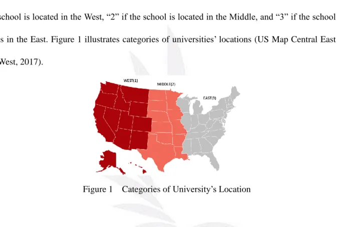
7. Location ( ). This is a dummy variable which tells the location in which the
university is situated in the United States. The dummy variable is equal to “1” if the
school is located in the West, “2” if the school is located in the Middle, and “3” if the school is in the East. Figure 1 illustrates categories of universities’ locations (US Map Central East West, 2017).
Figure 1 Categories of University’s Location
8. Selectivity ( ). This variable gives the acceptance rate (as a percentage) of the
university in 2016.
9. Calendar System ( ). This is a dummy variable which tells which academic term
the university follows. The dummy variable is equal to “0” if the school follows a quarter
system, and “1” if the school follows a semester system.
10. Funding Type ( ). This is a dummy variable which indicates whether the
school is private, and “1” if the school is public.
11. Ranking ( ). This is a dummy variable based on the university’s 2016 national
ranking from U.S. News & World Report (2017). The dummy variable is equal to “1” if
the university is ranked 1st -25th, “2” if the university is ranked 26th-50th, “3” if the university
is ranked 51st-75th, “4” if the university is ranked 76th-100th, “5” if the university is ranked
101st-200th, “6” if the university is ranked 201st-300th, and “7” if that the university is not in
the list of national ranking.
Data Analysis
The methodology of performing data analysis on factors affecting undergraduates’ starting salary is to apply SAS and R, and to fit the regression model based on the dataset that has been compiled. Techniques of the multiple regression analysis used in this study include creating scatter plots, displaying a correlation plot and matrix, generating a summary statistics table, and fitting multiple regression models. Then, model selection procedures are adopted to choose the best multiple regression models. Lastly, diagnostic checking and tests for assumptions are used to evaluate the best multiple regression model.
Specific procedures during the multiple regression analysis are described as follows:
1. Scatter plots: Eleven scatter plots are drawn to demonstrate the general relationship
between each explanatory variable and response variable. Data points that appear to deviate from the general pattern are pointed out and discussed.
2. Correlation plot and matrix: A correlation plot and a correlation matrix are drawn
and are designed to show the relationship among variables.
3. Summary statistics: Summary statistics, including number of observation, mean,
4. Full regression model: A full regression model with all 11 explanatory variables is
prepared. The regression model is shown in Equation 1 (Freund, Wilson, & Sa, 2006, p.74). The assumptions underlying this regression model include: (1) the mean of is 0; (2) the variance of is constant for all values of x; (3) the values of are independent; and (4) the error term follows a normal distribution (Anderson, Sweeney, Williams, Camm, &
Cochran, 2015, p.645). Adjusted , F test, and individual t tests are also stated and
discussed.
5. Model selection: According to Freund, Wilson, and Sa (2006), model selection based
on backward elimination, forward selection, stepwise regression, adjusted , Mallow’s ,
and Akaike information criterion (AIC, Akaike 1974) is performed: Backward elimination begins by considering all explanatory variables and eliminating the variable that contributes least to the model, then continues eliminating variables until all the remaining variables exceed the specified p-value and are all significant; forward selection begins with the best variable in the model and continues adding new variables in the model until no additional variables can sufficiently reduce the error mean square by the specified p-value; stepwise regression functions like forward selection at the beginning but allows elimination of one
variable before a new variable is added; the adjusted method lists all combinations of
regression models and regards as the best model the one that has the highest adjusted ;
similarly, the Mallow’s and AIC methods each lists all combinations of regression
models and regards as the best model the one that has the lowest and AIC value. The
0.15; the selection criterion for adjusted is 0.10; and the selection criteria for Mallow’s , and AIC are 0.20.
6. Refit best model: This procedure refits the model based on the selected variables from
the previous model selection procedure and checks whether or not the adjusted has
increased.
7. Diagnostic checks and tests for assumptions: According to Freund, Wilson, and Sa
(2006), three diagnostic checks should be performed to check for any outliers, leverage points, or influential observations. The first check is for outliers. The method of checking for outliers used in this study involves quantifying the studentized residual. Observations with residual values exceeding the criterion of 3 should be examined as possible outliers. The next check is for leverage points. The method of checking for leverage points used in this study involves searching for large leverage values. A leverage value is usually regarded as large if it is more than twice as large as the mean leverage value. The last check is for influential observations. The method of checking for influential observations used in this study involves calculating the Cook’s distance statistic. If Cook’s distance statistic is greater than 0.5, the data point may be influential. If Cook’s distance statistic is greater than 1, it is highly possible that the data point is influential. In addition to these three diagnostic checks, various tests were conducted to verify that the regression model follows Gaussian assumptions and that error terms are
independently, identically distributed, or .
Results
Relationship Between Each University-Related Factor and Starting Median Salary
Eleven scatter plots were drawn as shown below to demonstrate the general relationship between each explanatory variable and each response variable. This study tends to compare
San Jose State University with other U.S universities, because the author of this paper studies in the San Jose State University-FCU Dual-Degree Bachelor’s Program and seeks to provide information about this school that is useful to international students who may matriculate there. Consequently, observation 45 pertaining to San Jose State University (SJSU) is highlighted in the following scatter plots.
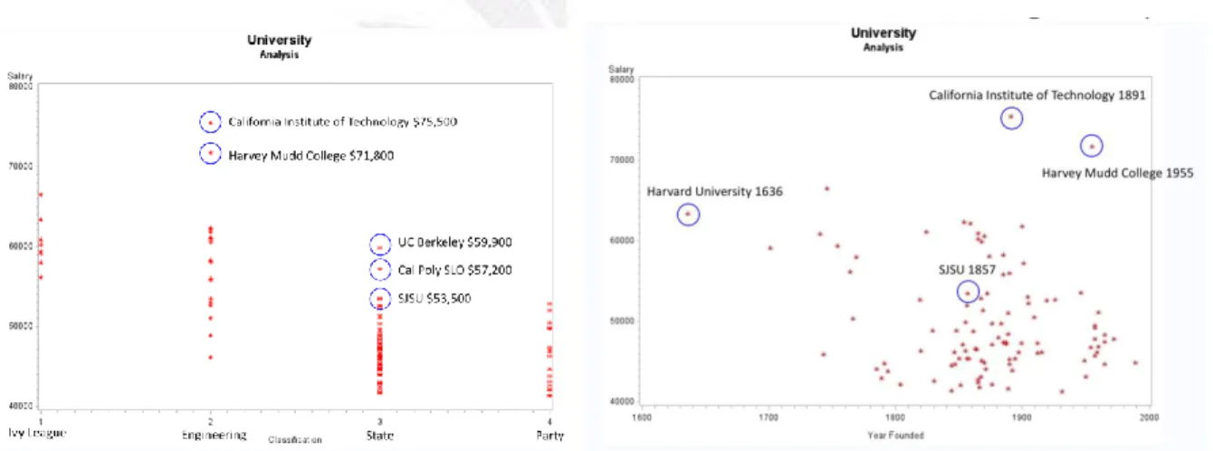
The left graph in Figure 2 presents the scatter plot of University Classification vs. Median Starting Salary. There appears to be significant grouping of data points for each school type depicted on the graph, indicating that the different types of school classified by Kaggle (2017) generally do have different starting salaries for their undergraduate students. The undergraduates from Ivy League schools generally have the highest salaries, followed by engineering schools, public schools (e.g. San Jose State University), and party schools, in that order. The right graph in Figure 2 presents the scatter plot of Year Founded vs. Median Starting Salary. This graph does not seem to have a significant, observable trend or pattern.
Figure 2 Classification & Year Founded vs. Median Starting Salary
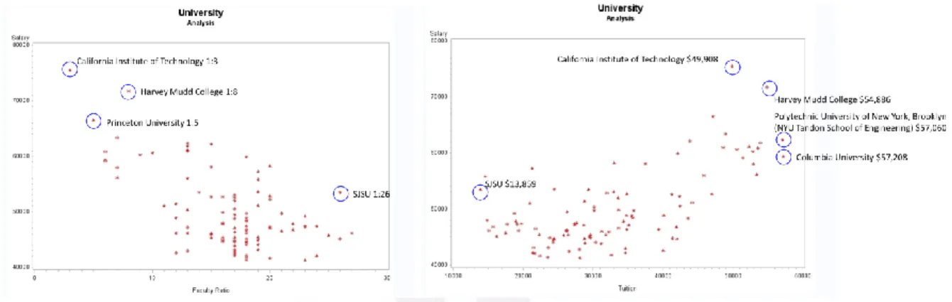
The left graph in Figure 3 presents the scatter plot of Student-Faculty Ratio vs. Median Starting Salary. There appears to be a downward trend which suggests that lower
student-faculty ratios at a university generally translate into higher starting salaries for that school’s undergraduates. The right graph in Figure 3 presents the scatter plot of Tuition vs. Median Starting Salary. There appears to be an upward trend in this graph, which suggests that undergraduates from universities that charge higher tuition obtain higher starting salaries than their counterparts from cheaper schools.
Figure 3 Student-Faculty Ratio & Tuition vs. Median Starting Salary
The left graph in Figure 4 presents the scatter plot of Enrollment vs. Median Starting Salary and the right graph in Figure 4 presents the scatter plot of Endowment vs. Median Starting Salary. There does not seem to be a significant, observable pattern or trend in either of these scatter plots.
Figure 4 Enrollment & Endowment vs. Median Starting Salary
Salary. It demonstrates that the two schools that have the highest starting salaries for undergraduates are located in the western region of the United States. The right graph in Figure 5 presents the scatter plot of Selectivity vs. Median Starting Salary. There appears to be a downward trend which indicates that universities with lower acceptance rates generally have higher starting salaries for their undergraduates.
Figure 5 Location & Selectivity vs. Median Starting Salary
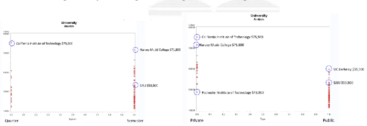
The left graph in Figure 6 presents the scatter plot of Calendar System vs. Median Starting Salary. No specific pattern is recognizable. However, the universities that follow the semester system appear to outnumber the universities that follow quarter system in this dataset. The right graph in Figure 6, Funding Type vs. Median Starting Salary, shows that private schools generally have higher starting salaries than public schools.
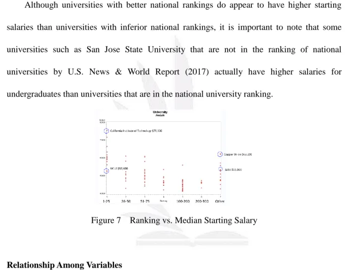
Figure 7 presents the scatter plot of Ranking vs. Median Starting Salary. It appears to have a downward trend, suggesting that a relationship exists between a school’s national rank according to U.S. News & World Report (2017) and the starting salaries of that university’s undergraduates. That is, the higher the university is ranked, the higher starting salaries its undergraduates can earn.
Although universities with better national rankings do appear to have higher starting salaries than universities with inferior national rankings, it is important to note that some universities such as San Jose State University that are not in the ranking of national universities by U.S. News & World Report (2017) actually have higher salaries for undergraduates than universities that are in the national university ranking.
Figure 7 Ranking vs. Median Starting Salary
Relationship Among Variables
Both the correlation plot and the correlation matrix are designed to demonstrate the correlation among variables and to verify the observed relationships in the scatter plots.
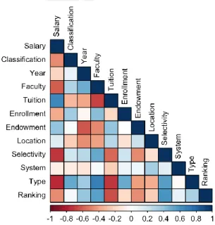
Figure 8 presents the correlation plot of the relationships among variables. The color of blue indicates that the variables have positive correlation, while the color of red indicates that the variables have negative correlation. The darker the color is, the stronger the correlation
that exists between the two variables. The first column of the plot is especially important, as it reveals the magnitude of correlation between explanatory variables and response variable. The explanatory variable Tuition and response variable Salary have strong positive correlation, while the explanatory variables Endowment and Location have weak positive correlation with the response variable Salary. By contrast, the explanatory variables Student-Faculty Ratio (Faculty), Selectivity, and Funding Type have strong negative correlation with the response variable Salary, and the explanatory variables Classification, Year Founded (Year), Enrollment, and Ranking have medium negative correlation with the response variable Salary. The explanatory variable System has barely any correlation with the response variable Salary.
In addition, other findings can be observed from the correlation plot, including a strong positive correlation between Funding Type and Student-Faculty Ratio as well as strong negative correlation between Funding Type and Tuition. These findings indicate that private schools usually are associated with high tuition and low student-faculty ratio.
Figure 8 Relationship among Variables
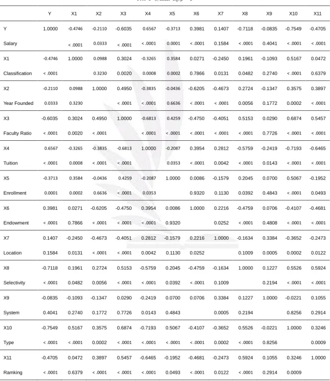
correlation matrix (shown in Table 1) gives the exact correlation coefficients and p-values for
testing whether . The results from the correlation matrix are same as the results
from correlation plot.
Table 1 Correlation Matrix among Variables
Pearson Correlation Coefficients, N=102 Prob |r| under Y X1 X2 X3 X4 X5 X6 X7 X8 X9 X10 X11 Y Salary 1.0000 -0.4746 < .0001 -0.2110 0.0333 -0.6035 < .0001 0.6567 < .0001 -0.3713 0.0001 0.3981 < .0001 0.1407 0.1584 -0.7118 < .0001 -0.0835 0.4041 -0.7549 < .0001 -0.4705 < .0001 X1 Classification -0.4746 < .0001 1.0000 0.0988 0.3230 0.3024 0.0020 -0.3265 0.0008 0.3584 0.0002 0.0271 0.7866 -0.2450 0.0131 0.1961 0.0482 -0.1093 0.2740 0.5167 < .0001 0.0472 0.6379 X2 Year Founded -0.2110 0.0333 0.0988 0.3230 1.0000 0.4950 < .0001 -0.3835 < .0001 -0.0436 0.6636 -0.6205 < .0001 -0.4673 < .0001 0.2724 0.0056 -0.1347 0.1772 0.3575 0.0002 0.3897 < .0001 X3 Faculty Ratio -0.6035 < .0001 0.3024 0.0020 0.4950 < .0001 1.0000 -0.6813 < .0001 0.4259 < .0001 -0.4750 < .0001 -0.4051 < .0001 0.5153 < .0001 0.0290 0.7726 0.6874 < .0001 0.5457 < .0001 X4 Tuition 0.6567 < .0001 -0.3265 0.0008 -0.3835 < .0001 -0.6813 < .0001 1.0000 -0.2087 0.0353 0.3954 < .0001 0.2812 0.0042 -0.5759 < .0001 -0.2419 0.0143 -0.7193 < .0001 -0.6465 < .0001 X5 Enrollment -0.3713 0.0001 0.3584 0.0002 -0.0436 0.6636 0.4259 < .0001 -0.2087 0.0353 1.0000 0.0086 0.9320 -0.1579 0.1130 0.2045 0.0392 0.0700 0.4843 0.5067 < .0001 -0.1952 0.0493 X6 Endowment 0.3981 < .0001 0.0271 0.7866 -0.6205 < .0001 -0.4750 < .0001 0.3954 < .0001 0.0086 0.9320 1.0000 0.2216 0.0252 -0.4759 < .0001 0.0706 0.4808 -0.4107 < .0001 -0.4681 < .0001 X7 Location 0.1407 0.1584 -0.2450 0.0131 -0.4673 < .0001 -0.4051 < .0001 0.2812 0.0042 -0.1579 0.1130 0.2216 0.0252 1.0000 -0.1634 0.1009 0.3384 0.0005 -0.3652 0.0002 -0.2473 0.0122 X8 Selectivity -0.7118 < .0001 0.1961 0.0482 0.2724 0.0056 0.5153 < .0001 -0.5759 < .0001 0.2045 0.0392 -0.4759 < .0001 -0.1634 0.1009 1.0000 0.1227 0.2194 0.5526 < .0001 0.5924 < .0001 X9 System -0.0835 0.4041 -0.1093 0.2740 -0.1347 0.1772 0.0290 0.7726 -0.2419 0.0143 0.0700 0.4843 0.0706 0.3384 0.0005 0.1227 0.2194 1.0000 -0.0221 0.8256 0.1055 0.2914 X10 Type -0.7549 < .0001 0.5167 < .0001 0.3575 0.0002 0.6874 < .0001 -0.7193 < .0001 0.5067 < .0001 -0.4107 < .0001 -0.3652 0.0002 0.5526 < .0001 -0.0221 0.8256 1.0000 0.3246 0.0009 X11 Ramking -0.4705 < .0001 0.0472 0.6379 0.3897 < .0001 0.5457 < .0001 -0.6465 < .0001 -0.1952 0.0493 -0.4681 < .0001 -0.2473 0.0122 0.5924 < .0001 0.1055 0.2914 0.3246 0.0009 1.0000
Summary Statistics for Each Variable
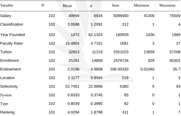
Table 2 illustrates the mean, standard deviation, sum, minimum value, and maximum value of each variable among the 102 universities in 2016. For example, the average value (i.e., mean) of each variable among the 102 universities in 2016 can be found in Table 2 as follows:
The average undergraduates’ starting median salary is $49,994; the average student-faculty ratio is about 1:16.5; the average tuition is $32,853; the average enrollment is 25291 students; the average endowment is 2.01964 billion U.S. Dollars, and the average acceptance rate is about 52.75% .
Table 2 Summary Statistics for Each Variable
Variable N Sum Minimum Maximum Salary 102 49994 6934 5099400 41300 75500 Classification 102 3.0588 1.2091 312 1 4 Year Founded 102 1872 62.1325 190929 1636 1989 Faculty Ratio 102 16.4804 4.7151 1681 3 27 Tuition 102 32853 11219 3351023 13859 57208 Enrollment 102 25291 14809 2579726 829 65302 Endowment 102 2.0196 4.9808 206.00330 0.01040 35.7 Location 102 2.1177 0.8594 216 1 3 Selectivity 102 52.7451 22.9898 5380 5 93 System 102 0.8333 0.3745 85 0 1 Type 102 0.8039 0.3990 82 0 1 Ranking 102 4.0294 1.8798 411 1 7
Relationship Between Eleven University-Related Factors and Starting Median Salary
The result of the full regression model is shown in Table 3 and Table 4.
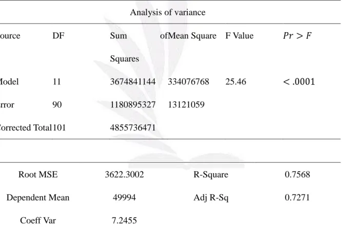
Table 3 shows that the adjusted is 0.7271 in the regression model. This means that
72.71% of the variability in undergraduates’ starting median salary can be explained by the linear relationship between the 11 explanatory variables and the starting median salary. Next, the p-value from the F test is smaller than 0.0001, suggesting that, overall, there is a significant relationship between the 11 explanatory variables and the starting median salary.
Table 3 Analysis of Variance in Full Regression Model Analysis of variance
Source DF Sum of
Squares
Mean Square F Value
Model 11 3674841144 334076768 25.46
Error 90 1180895327 13121059
Corrected Total 101 4855736471
Root MSE 3622.3002 R-Square 0.7568
Dependent Mean 49994 Adj R-Sq 0.7271
Coeff Var 7.2455
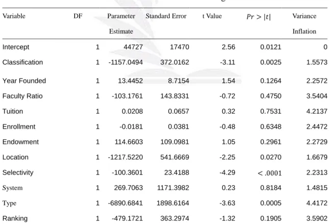
While the F test shows that the multiple regression relationship is significant, the t-test on individual parameters in Table 4 shows that the variables Year Founded, Student-Faculty Ratio, Tuition, Enrollment, Endowment, Calendar System, and Ranking have their respective
Thus, the variables Year Founded, Student-Faculty Ratio, Tuition, Enrollment, Endowment, System, and Ranking do not have a significant relationship with the response variable (Starting Median Salary) in this full regression model. For the reamining parameters (Classification, Location, Selectivity, Funding Type), their p-values are all less than based on their individual t-test and thus the parameters are significant in this model.
According to Freund, Wilson, and Sa (2006), multicollinearity exists whenever there are strong correlations among explanatory variables in the regression model. If it exists, it can distort the analytic results. To diagnose multicollinearity, the value of variance inflation factor (VIF) is considered. Since the largest value of VIF in the full regression model is 4.21366 (as shown in Table 4) and is smaller than the criterion of 10, there is no multicollinearity in the full model.
Table 4 Parameter Estimates of Full Regression Model
Variable DF Parameter Estimate
Standard Error t Value Variance Inflation Intercept 1 44727 17470 2.56 0.0121 0 Classification 1 -1157.0494 372.0162 -3.11 0.0025 1.5573 Year Founded 1 13.4452 8.7154 1.54 0.1264 2.2572 Faculty Ratio 1 -103.1761 143.8331 -0.72 0.4750 3.5404 Tuition 1 0.0208 0.0657 0.32 0.7531 4.2137 Enrollment 1 -0.0181 0.0381 -0.48 0.6348 2.4472 Endowment 1 114.6603 109.0981 1.05 0.2961 2.2729 Location 1 -1217.5220 541.6669 -2.25 0.0270 1.6679 Selectivity 1 -100.3601 23.4188 -4.29 2.2313 System 1 269.7063 1171.3982 0.23 0.8184 1.4815 Type 1 -6890.6841 1898.6164 -3.63 0.0005 4.4172 Ranking 1 -479.1721 363.2974 -1.32 0.1905 3.5902
Five Variables as the Best Model
The criteria for model selection in this study include backward elimination, forward
selection, stepwise regression, adjusted , Mallow’s , and AIC. Table 5 shows the results
of variable selection based on 6 different criteria. All criteria except adjusted select
variables Classification, Location, Selectivity, Type, and Ranking as the best model. Only the
adjusted criterion indicates that the best model includes Classification, Year Founded,
Faculty Ratio, Endowment, Location, Selectivity, Type, and Ranking. Table 5 Model Selection Summary
Selection
procedures
Classification Year Founded Faculty Ratio Tuition Enrollment Endowment Location Selectivity System Type Ranking Selection
Criteria Backward Elimination ✓ ✓ ✓ ✓ ✓ 0.15 Forward Selection ✓ ✓ ✓ ✓ ✓ 0.15 Stepwise Regression ✓ ✓ ✓ ✓ ✓ 0.15 Adjusted R-Square ✓ ✓ ✓ ✓ ✓ ✓ ✓ ✓ 0.10 Mallow’s Cp ✓ ✓ ✓ ✓ ✓ 0.20 AIC ✓ ✓ ✓ ✓ ✓ 0.20
Since backward elimination, forward selection, stepwise regression, Mallow’s , and
AIC all select variables Classification, Location, Selectivity, Type, and Ranking as the best model, these five variables will be used to refit the best regression model (see Equation 2).
,where (2)
The analysis of variance and parameter estimates of the best regression model is shown in Table 6 and Table 7. Comparing the new regression model with the full model, the adjusted slightly increases from 0.7271 to 0.7330. Table 6 shows that, in new model, 73.31% of the variability in undergraduate starting median salary can be explained by the linear
relationship between the selected 5 explanatory variables and the starting median salary. The p-value from the F test is still smaller than 0.0001, suggesting there is an overall significant relationship between the starting median salary and the 5 explanatory variables. Furthermore, the t-test on the individual parameters shows that all five explanatory variables have their
p-values less than . Thus, the individual t-tests also indicate that the five parameters
are significant in this new regression model.
Table 6 Analysis of Variance of Best Regression Model Analysis of variance
Source DF Sum of
Squares
Mean Square F Value
Model 5 3623257146 724651429 56.44
Error 96 1232479325 12838326
Corrected Total 101 4855736471
Root MSE 3583.0610 R-Square 0.7462
Dependent Mean 49994 Adj R-Sq 0.7330
Coeff Var 7.1670
Table 7 demonstrates that five parameter estimates are negative, indicating that the explanatory variables Classification, Location, Selectivity, Funding Type, and Ranking have a negative relationship with the starting median salary. For the variable Classification, the coefficient is -1118.1977, meaning that for each increase in value of this dummy variable, the starting median salary for undergraduates decreases $1118.1977. Ivy League schools, labeled
as 1 in this dummy variable, generally have the highest starting median salaries for undergraduates, followed by engineering schools (labeled as 2 in the dummy variable) and public schools (labeled as 3 in the dummy variable). As the value of the dummy increases, the salary decreases at a rate of 1118.1977, with “party schools” having the lowest starting median salaries for their undergraduates. For the variable Location, the coefficient is -1396.4231, meaning that undergraduates from universities in the western region of the United States have, on average, a median starting salary this is $1396.4231 higher than the median starting salary for undergraduates from universities in the eastern region of the United States. For the variable Selectivity, the coefficient is -107.8531, meaning that, for a one percent decrease in acceptance rate, the starting median salary increases $107.8531. For the variable Funding Type, the coefficient is -8252.6270, meaning that undergraduates from private schools have, on average, a median starting salary that is $8252.6270 higher than the amount received by their public school counterparts. Finally, for the variable Ranking, the coefficient is -509.4506, meaning that the starting median salary for undergraduates increases $509.4506 for every decrease in value of the dummy variable. For example, universities that
are ranked in tier 1 (1st-25th place) typically have $509.4506 higher starting median salary
than universities that are ranked in tier 2 (25th-50th place).
In addition, since the largest value of VIF in the best regression model is 2.0643 and is smaller than 10 (shown in Table 7), there is no multicollinearity in the best model.
Table 7 Parameter Estimates of Best Regression Model
Variable DF Parameter Estimate
Standard Error t Value Variance Inflation Intercept 1 70748 1848.6802 38.27 0 Classification 1 -1118.1977 350.1866 -3.19 0.0019 1.4103 Location 1 -1396.4231 457.3798 -3.05 0.0029 1.2154 Selectivity 1 -107.8531 22.1141 -4.88 2.0334 Type 1 -8252.6270 1283.8648 -6.43 2.0643 Ranking 1 -509.4506 241.9765 -2.11 0.0379 1.6278
Diagnostic Checks and Tests for Assumptions
Three diagnostic checks and various tests for assumptions were used to evaluate the best multiple regression model. The search for outliers was the first diagnostic check. Table 8 shows that the largest studentized residual (in absolute value) is 3.0175 from observation 46, which slightly exceeds the criterion of 3. Observation 46, which represents South Dakota School of Mines and Technology, is the only outlier in the dataset. As a school with one of the highest starting salaries for undergraduates in the central part of the United States (see the left graph in Figure 5 Location & Selectivity vs. Median Starting Salary), South Dakota School of Mines and Technology is an outlier since the observation pertaining to it deviates from the trend in the scatter plot of Selectivity vs. Starting Median Salary (see the right graph in Figure 5). Although the school has a high acceptance rate of 85%, it also has a relatively high starting median salary of $55,800 for its undergraduates.
Table 8 Diagnostic Checking on Observation 46
Observation Residual RStudent Hat Diag H Cov
Ratio
DEFITS DFBETAS
Intercept X1 X7 X8 X10 X11
The second diagnostic check sought out influential observations. Because none of the observations had a Cook’s Distance greater than 0.5 (observation 6 had a Cook’s D of 0.165, the largest in the dataset), this study determined that the dataset does not contain any influential observations.
The third and final diagnostic check determined if any leverage points exist. By
checking leverage values (Criterion: ), the study
determined that there are a total of 11 leverage points among the 102 observations: (i) Observation 5 (California Polytechnic State University-San Luis Obispo), (ii) Observation 6 (California Institute of Technology), (iii) Observation 10 (California State University, Long Beach), (iv) Observation 14 (Colorado School of Mines), (v) Observation 16 (Cooper Union), (vi) Observation 19 (Embry-Riddle Aeronautical University), (vii) Observation 22 (Georgia Institute of Technology), (viii) Observation 24 (Harvey Mudd College), (ix) Observation 30 (New Mexico Institute of Mining and Technology), (x) Observation 36 (Polytechnic University of New York, Brooklyn), and (xi) Observation 99 (Wentworth Institute of Technology).
To evaluate the best multiple regression model, various tests for 4 assumptions were performed as follows:
Assumption 1. This study tested whether , the test for location. Table 9 indicates that, since the p-value for Student’s t is 0.9736 and is greater than α=0.05, the test statistic fails to reject the null hypothesis of µ=0. Thus, the regression model satisfies the
Table 9 Tests for Location
Tests for Location: =0
Test Statistic p Value
Student’s t t 0.0332 Pr > |t| 0.9736
Sign M -2 Pr >= |M| 0.7666
Signed Rank S -61.5 Pr >= |S| 0.8385
Assumption 2. The next analysis tests whether . Anderson, Sweeney, Williams, Camm, and Cochran (2015) point out that the residual versus predicted value plot is used to check that the variance of the error term is constant for all values of x, and that the residual plot should look like a horizontal band on points with no specific pattern if the assumption is satisfied. From the residual plot in Figure 9, there does not seem to be a specific pattern, verifying the assumption that the variance of ε is the same for all values of x.
Hence, the regression model satisfies the assumption .
Assumption 3. This study also tested the assumption . Montgomery, Peck, and Vining (2012) mentioned that the Durbin-Watson Statistics tests whether autocorrelation exists and whether the residuals from the multiple regression are independent. Two hypotheses are:
The Durbin-Watson Statistics indicate the p-vales are 0.1448 and 0.8552 and are both
greater than α=0.05. Thus, the test statistic fails to reject the null hypothesis of .
Hence, the regression model satisfies the assumption .
Assumption 4. Four separate tests are used for the assumption , the test for normality. The Shapiro-Wilk test, Kolmogorov-Smirnov test, Cramer-von Mises test, and Anderson-Darling test are used to test whether the error term follows a normal distribution. The results of normality tests in Table 10 reveal that, while all the tests have p-values exceeding α=0.05 (the smallest p-value among 4 tests is 0.1500), the test statistics fail to reject the null hypothesis that the distribution is normal. As a result, the regression model
satisfies the assumption .
Table 10 Tests for Normality Tests for Normality
Test Statistic p Value
Shapiro-Wilk W 0.9921 Pr < W 0.8175
Kolmogorov-Smirnov D 0.0537 Pr > D >0.1500
Cramer-von Mises W-Sq 0.0461 Pr > W-Sq >0.2500
Summary of Results
This study aims to explore what university-related factors affect undergraduate students’ starting salaries after their graduation in the United States. Eleven factors drawn from 102 U.S. universities were analyzed throughout this study, including each school’s classification, year founded, average student-faculty ratio, tuition, total number of students enrolled, endowments provided, location, acceptance rate, system of academic term, funding type (e.g., private/public), and ranking.
Results of the study indicate that not all of the 11 university-related factors can be used to explain the starting median salaries for undergraduates from different universities in the United States. Five of the university-related factors (classification, location, acceptance rate, funding type, and ranking) have a significant relationship with undergraduates’ starting median salaries, while the other 6 university-related factors (year founded, student-faculty ratio, tuition, enrollment, endowment, and type of academic term) do not. Results of the study further show that undergraduate students who graduate from private, top-ranked universities in the western region of the United States that primarily focus on engineering schools and have a low acceptance rate generally have higher starting salaries than students who graduate from other universities in the United States.
Discussion Significant Factors for Choosing U.S. Universities
While universities have many attributes that may affect their undergraduate students’ starting salaries, the results of this study provide a broad survey of several university-related factors that have a statistically significant impact on starting salaries, and may serve as a reference for prospective undergraduates. If prospective undergraduates who plan to attend a
U.S. university are concerned about their future salaries, they can check the classification, location, acceptance rate, funding type, and ranking each university they are considering and refer to the results of this study.
According to the results of this study, undergraduate students who graduate from private, top-ranked universities in the western region of the U.S. that primarily focus on engineering and have a low acceptance rate generally have higher starting salaries than students who graduate from other universities. For example, undergraduates from universities in the western region of the United States have a starting median starting salary that, on average, is $1396.42313 higher than the starting median salary received by undergraduates from universities in the eastern region of the United States. Moreover, recent graduates from universities ranked in the top 25 nationally typically have a median starting salary that is $509.45058 higher than the median starting salary of recent graduates from universities that
ranked in 25th-50th place.
According to the 2018-2018 College Salary Report published by PayScale (2017), the universities whose undergraduates obtain the highest starting salaries after graduation are mostly located in the state of California. The results of the Payscale study agree with the analytic result of this study, which finds that the location of a university affects its undergraduates’ starting salaries. Undergraduates from universities in the western part of the United States typically have higher starting salaries than undergraduates from universities in the east. Universities in the state of California in the western United States have high starting salaries for their undergraduates.
Merits of San Jose State University
study (Ranking vs. Median Starting Salary), which shows that, even though San Jose State University is not ranked among the national universities, its undergraduates actually have higher starting salaries than their counterparts from universities that are in the national university ranking. As this study has indicated, a school’s ranking is not the only university-related factor that affects its undergraduates’ future salary. Prospective students should concurrently consider other factors when they seek to choose universities that can bring more wealth to them.
Further comparison of the sample average (mean) data in Table 2 (Summary Statistics for Each Variable) with the statistics of San Jose State University shows that San Jose State University is actually a school with a high return of investment (ROI). Table 11 gives the comparison between San Jose State University (SJSU) and a national sample mean of the dataset used in this study. While San Jose State University’s tuition of $13,859 is significantly cheaper than the sample’s average of $32,853, the starting median salary for San Jose State University’s undergraduates is $53,500 and is well above the national sample average of $49,994. This result implies that students who study at San Jose State University “invest” little to get a high potential return from salary. For prospective students who will study at San Jose State University, this study reinforces the merits of the university based on its affordability and high return on investment.
Table 11 Comparison between SJSU and National Sample Average
Variables National Sample Average San Jose State University
Tuition $32,853 $13,859
Student-Faculty Ratio 1:16.4804 1:26
Enrollment 25,291 34,618
Endowment (in billions) $2.0196 $0.1256
Selectivity 52.7451% 53%
Mean Starting Salary $49,994 $53,500
Limitations of the Study
Although the results of the regression model in this study describe the general relationship between variables, it is important to note the limitations of this study. First,
because the adjusted is 0.7330, the regression model can only explain about 73% of the
observations’ variability. There are still certain observations that cannot be explained by the estimated regression line. Next, while there are 5 significant explanatory variables (factors) in the best model, there are other variables that can possibly explain undergraduates starting median salaries. These variables that are not identified in this study can influence the estimated regression line. Also, because only 102 universities across the United States are included within the sample used in this study, the sample results may deviate from the results that would be obtained had the study assessed the entire population. Lastly, the response variable in this study is based on undergraduates’ starting median salary. However, in reality, different students who graduate and receive bachelor degrees from the same university can still have varying salaries based on their majors. For example, it has been observed in this
study that students who graduate from schools that emphasize engineering have higher starting salaries than others. So, students who graduate from an engineering program of a university typically can earn higher salaries than students who graduate from other programs of the same university. In this case, the regression model in this study cannot indicate such variations.
Conclusion
The purpose of this study is to investigate what university-related factors can determine undergraduate students’ starting salaries in the United States. What has been learned in this study is that certain university-related factors (classification, location, acceptance rate, funding type, and ranking) affect undergraduates’ starting salaries. In addition, choosing a private, top-ranked university in the western part of the United States that primarily focuses on engineering and has a low acceptance rate increases undergraduates’ chances of getting high a starting salary after graduation. For prospective students who will study in the United States for bachelor’s degree, this study offers them practical information about what university-related factors can be used to estimate their starting salaries after graduation. This study also helps them choose universities that can potentially yield higher salaries in the future.
References
Akaike, H. (1974), A new look at the statistical model identification", IEEE Transactions on Automatic Control, 19, 716–723.
Anderson, D. R., Sweeney, D. J., Williams, T. A., Camm, J. D., & Cochran, J. J. (2015).
Statistics for business and economics. Singapore: Cengage Learning
Freund, R. J., Wilson, W. J., & Sa, P. (2006). Regression analysis: Statistical modeling of a
response variable. Singapore: Elsevier
Kaggle (2017, December 23). Where it pays to attend college. Retrieved from https://www.Kaggle(2017).com/wsj/college-salaries
Montgomery, D. C., Peck, E. A., & Vining, G. G. (2012). Introduction to linear regression
analysis. Retrieved from https://books.google.com.tw/
PayScale (2017, December 23). 2017-2018 College Salary Report. Retrieved from https://www.PayScale(2017).com/college-salary-report
US Map Central East West (2017, December 23). Retrieved from http://thempfa.org/us-map- central-east-west/us-map-central-east-west-1200px-us-west-map/
U.S. News & World Report (2017, December 23). National university rankings. Retrieved from https://www.usnews.com/best-colleges/rankings/national-universities
Appendix A
Dataset for the Study
School Name Salary Classification Year Faculty Tuition Enrollment Endowment Location Selectivity System Type Ranking
Arizona State University (ASU) 47400 2 1885 23 27372 51869 0.4839 1 83 1 1 5
Auburn University 45400 4 1856 19 29640 28290 0.6576 2 81 1 1 5
Binghamton University 53600 4 1946 19 24403 17292 0.0934 3 41 1 1 4
Brown University 56200 3 1764 7 53419 9781 3 3 9 1 0 1
Cal Poly San Luis Obispo 57200 4 1901 19 21312 21306 0.1904 1 29 0 1 7
California Institute of Technology (CIT) 75500 1 1891 3 49908 2240 2.2 1 8 0 0 1
California State University (CSU), Chico 47400 4 1887 24 19779 17557 0.0493 1 67 1 1 7
California State University, East Bay (CSUEB) 49200 4 1957 23 18714 15855 0.017 1 70 0 1 7
California State University, Fullerton (CSUF) 45700 4 1957 25 17460 40235 0.0589 1 48 1 1 6
California State University, Long Beach (CSULB) 45100 4 1949 26 16196 37776 0.0566 1 32 1 1 7
California State University, Sacramento (CSUS) 47800 4 1957 22 18918 9762 0.0104 1 74 1 1 7
Carnegie Mellon University (CMU) 61800 1 1900 13 53910 13961 1.3 3 22 1 0 1
Clemson University 48400 4 1889 18 35654 23406 0.6213 3 51 1 1 3
Colorado School of Mines 58100 1 1874 15 37436 5876 0.2123 1 40 1 1 3
Columbia University 59400 3 1754 6 57208 25084 9 3 6 1 0 1
Cooper Union 62200 1 1859 15 43850 964 0.738 3 13 1 0 7
Cornell University 60300 3 1865 9 52853 22319 5.8 3 14 1 0 1
Dartmouth College 58000 3 1769 7 52950 6409 4.5 3 11 0 0 1
Embry-Riddle Aeronautical University (ERAU) 52700 1 1926 16 34822 6011 0.074 3 71 1 0 7
Florida State University (FSU) 42100 2 1851 24 21673 41368 0.5845 3 58 1 1 4
George Mason University 47800 4 1972 16 34370 34904 0.0716 3 81 1 1 5
Georgia Institute of Technology 58300 1 1885 20 33014 26839 1.8 3 26 1 1 2
Harvard University 63400 3 1636 7 48949 20324 35.7 3 5 1 0 1
Harvey Mudd College 71800 1 1955 8 54886 829 0.276 1 13 1 0 1
Illinois Institute of Technology (IIT) 56000 1 1890 13 45864 7730 0.2242 2 57 1 0 5
Indiana University (IU), Bloomington 46300 2 1820 17 34845 49695 0.9911 2 79 1 1 4
Iowa State University 45400 4 1858 19 22256 36350 0.6994 2 87 1 1 5
Louisiana State University (LSU) 46900 2 1960 18 15708 3277 0.0162 2 31 1 1 5
Michigan State University (MSU) 46300 4 1855 17 39405 50344 2.6 2 66 1 1 4
(New Mexico Tech)
North Carolina State University (NCSU) 47200 4 1887 13 27406 33755 0.9986 3 46 1 1 4
Ohio State University (OSU) 44900 4 1870 19 29659 59482 3.7 2 54 1 1 3
Ohio University 42200 2 1804 18 21360 29712 0.4848 2 75 1 1 5
Oregon State University (OSU) 45100 4 1868 18 29457 30354 0.5628 1 77 0 1 5
Pennsylvania State University (PSU) 49900 2 1855 16 33664 47789 1.8 3 56 1 1 3
Polytechnic University of New York, Brooklyn 62400 1 1854 13 57060 5212 0.121 3 35 1 0 7
Princeton University 66500 3 1746 5 47140 8181 21.7 3 7 1 0 1
Purdue University 51400 4 1869 12 28804 40451 2.2 2 56 1 1 3
Randolph-Macon College 42600 2 1830 12 40000 1446 0.1434 3 61 0 1 7
Rensselaer Polytechnic Institute (RPI) 61100 1 1824 13 52305 7442 0.632 3 44 1 0 2
Rochester Institute of Technology (RIT) 48900 1 1829 12 40068 15353 0.7509 3 55 1 0 4
Rutgers University 50300 4 1766 13 30203 50146 0.8659 3 57 1 1 3
San Diego State University (SDSU) 46200 4 1897 27 19340 34688 0.2232 1 35 1 1 5
San Francisco State University (SFSU) 47300 4 1899 23 19134 29045 0.0468 1 68 1 1 6
San Jose State University (SJSU) 53500 4 1857 26 13859 34618 0.1256 1 53 1 1 7
South Dakota School of Mines & Technology 55800 1 1885 19 14580 2859 0.0537 2 85 1 1 7
State University of New York (SUNY) at Albany 44500 4 1844 18 24358 17373 0.0593 3 54 1 1 5
State University of New York (SUNY) at Buffalo 46200 4 1846 13 26270 30183 0.601 3 59 1 1 4
State University of New York (SUNY) at
Farmingdale
47300 4 1912 20 17726 9235 0.052 3 58 1 1 7
Stevens Institute of Technology 60600 1 1870 10 50554 6523 0.166 3 39 1 0 3
Stony Brook University 49500 4 1957 17 26297 25734 0.2197 3 41 1 1 4
Tennessee Technological University 46200 1 1915 18 26190 10492 0.0529 2 67 1 1 6
Texas A&M University 49700 4 1876 21 30208 65302 9.9 2 66 1 1 3
University of Alabama at Huntsville (UAH) 43100 4 1950 17 21480 8468 0.0751 2 76 1 1 6
University of Alabama, Tuscaloosa 41300 2 1931 23 28100 37663 0.6832 2 53 1 1 5
University of Arkansas 44100 4 1871 19 24308 27194 0.8989 2 63 1 1 5
University of California at Los Angeles (UCLA) 52600 4 1919 17 41270 44947 3.9 1 18 0 1 1
University of California, Berkeley 59900 4 1868 18 42112 40174 4.1 1 16 1 1 1
University of California, Davis 52300 4 1905 20 42396 36441 1.1 1 42 0 1 2
University of California, Irvine (UCI) 48300 4 1965 18 43530 32754 0.6259 1 41 0 1 2
University of California, Riverside (UCR) 46800 4 1954 22 41931 22921 0.2949 1 66 0 1 5
University of California, Santa Barbara (UCSB) 50500 2 1909 17 42423 24346 0.4292 1 36 0 1 2
University of California, Santa Cruz (UCSC) 44700 4 1965 18 42042 18783 0.2444 1 59 0 1 4
University of Colorado - Boulder (UCB) 47100 4 1876 17 35079 33771 0.5142 1 77 1 1 4
University of Colorado - Denver 46100 4 1912 15 31209 23960 0.4287 1 61 1 1 6
University of Connecticut (UConn) 48000 4 1881 16 14880 27721 0.3586 3 49 1 1 3
University of Delaware 45900 4 1743 15 32250 22168 1.3 3 65 0 1 4
University of Florida (UF) 47100 2 1853 20 28658 52367 1.5 3 46 1 1 2
University of Georgia (UGA) 44100 4 1785 18 30392 36574 1 3 54 1 1 3
University of Idaho 44900 4 1989 16 23812 11780 0.2375 1 76 1 1 5
University of Illinois at Chicago 47500 4 1965 18 27672 29120 0.3183 2 74 1 1 5
University of Illinois at Urbana-Champaign
(UIUC)
52900 2 1867 20 31988 46951 1.6 2 60 1 1 3
University of Iowa (UI) 44700 2 1847 16 28813 32011 1.3 2 84 1 1 4
University of Kansas 42400 4 1865 17 26592 27565 1.5 2 93 1 1 5
University of Kentucky (UK) 42800 4 1865 17 28046 29781 1.2 2 91 1 1 5
University of Maryland, College Park 52000 2 1856 17 33606 39083 0.4933 3 48 1 1 3
University of Massachusetts (UMass) - Amherst 46600 4 1863 18 33662 30037 0.2872 3 60 1 1 3
University of Massachusetts (UMass) - Lowell 45400 4 1894 17 31865 17854 0.0731 3 60 1 1 5
University of Minnesota 46200 4 1959 12 15092 1771 0.0128 2 58 1 1 3
University of Mississippi 41400 2 1844 18 23554 23610 0.6029 2 78 1 1 5
University of Nevada, Reno (UNR) 46500 4 1864 21 21787 21363 0.2852 1 83 1 1 6
University of New Hampshire (UNH) 41800 4 1866 18 32637 15236 0.3301 3 76 1 1 5
University of New Mexico (UNM) 41600 4 1889 20 22412 27060 0.3932 1 47 1 1 5
University of North Carolina at Chapel Hill
(UNCH)
42900 4 1789 13 34588 29469 2.9 3 27 1 1 2
University of Oklahoma 44700 4 1890 17 24443 31176 1 2 71 1 1 4
University of Oregon 42200 4 1876 17 34611 23546 0.7587 1 78 0 1 5
University of Pennsylvania 60900 3 1740 6 53534 21826 10.7 3 9 1 0 1
University of Rhode Island (URI) 43900 4 1892 17 28874 17834 0.1368 3 71 1 1 5
University of Tennessee 43800 2 1794 17 31160 28052 0.6546 2 77 1 1 5
University of Texas (UT) - Austin 49700 2 1883 18 35766 51331 3.4 2 40 1 1 3
University of Utah 45400 4 1850 16 26408 31860 0.958 1 76 1 1 5
University of Vermont (UVM) 44800 4 1791 17 41356 13105 0.4089 3 69 1 1 4
University of Washington (UW) 48800 4 1861 17 35538 45591 3 1 45 0 1 3
University of Wisconsin (UW) - Madison 48900 4 1848 18 34782 43336 3.1 2 53 1 1 2
Virginia Polytechnic Institute and State University
(Virginia Tech)
53500 1 1872 14 29371 33170 0.8358 3 71 1 1 3
Washington State University (WSU) 45300 4 1890 15 25817 30142 0.9078 1 72 1 1 5
Wentworth Institute of Technology 53000 1 1904 17 32954 4186 0.0841 3 71 1 0 7
West Virginia University (WVU) 43100 2 1867 19 23616 28488 0.5787 3 76 1 1 5
Worcester Polytechnic Institute (WPI) 61000 1 1865 13 48628 6642 0.4663 3 48 0 0 3