考慮內生性與樣本選擇之生產邊界估計方法—關聯結構法與共同邊界法之應用 - 政大學術集成

全文

(1)國立政治大學商學院金融學系博士論文 Department of Money and Banking College of Commerce. National Chengchi University Doctoral Dissertation. 考慮內生性與樣本選擇之生產邊界估計方法— 政治. 大. 立關聯結構法與共同邊界法之應用. ‧ 國. 學. An Estimation of Production Frontiers Taking Account of. ‧. Endogeneity and Selection under the Framework of. n. al. er. io. sit. y. Nat. Copula Methods and Metafrontier Models. Ch. engchi. i n U. v. 指導教授：黃台心博士研究生：謝子雄撰. 中華民國一○二年七月 July, 2013.

(2) 立. 政治大. ‧. ‧ 國. 學. n. er. io. sit. y. Nat. al. Ch. engchi. i n U. v.

(3) An Estimation of Production Frontiers Taking Account of Endogeneity and Selection under the Framework of Copula Methods and Metafrontier Models. National Chengchi University. 學 ‧. ‧ 國. 治政 Department of Money and大 Banking 立. n. al. er. io. sit. y. Nat. By. Zixiong Xie. Ch. engchi. i n U. v. July 1, 2013. Advising Professor: Dr. Tai-Hsin Huang.




(7) 謝辭為了等寫謝辭的這一天，我花了整整七年的時間，這箇中滋味，唯有自知。在這過程中，受許多師長幫忙。其中，我最要感謝黃台心老師的論文指導，引領我進入學術研究的大門。感謝口試委員 (王泓仁老師、胡均立老師、陳坤銘老師及林建秀老師) 的意見讓我的論文更加完善。沈中華老師的提攜與陳仕偉老師的鼓勵是讓我前行的動力。另外，我要特別感謝徐士勛老師對我的照顧與經濟上的支持，讓我在求學的過程中無後顧之憂。班上同學的陪伴，也讓漫長且苦悶的日子添加一些快樂。. 政治大為了求取博士學位，我花了七年時間。而我未來的老婆—莊佳樺，則花了整立. 整十五年只為了等我完成學業。家人則等了我三十三年，我才能開始為家裡付出. ‧ 國. 學. 一些心力。家人的陪伴與支持，是我最大的後盾與力量。最後，我將此論文獻給我最為思念的父親。. ‧. n. er. io. sit. y. Nat. al. Ch. engchi. i n U. v.


(9) Abstract Plants in Taiwan’s manufacturing are characterized as small- and medium-size with frequent exit and entry and the scale of survivors varies considerably with business cycles. Plants’ choices on whether to exit or to stay and continuing plants’ options on input quantities count on both technical efficiency and productivity. This entails a selection and a simultaneity problems in the estimation of production frontiers. This dissertation proposes a new approach to solve both issues under the. 政治大 and Petrin’s (2003) approaches. framework of the stochastic frontier approach. More specific, we extend Olley and Pakes’ (1996) and Levinsohn. 立. to a stochastic. production frontier and use copula methods to deal with simultaneity and selection at. ‧ 國. 學. the same time. Based on the proposed method, we further conduct a metafrontier analysis to compare the technical efficiency and technology gap ratio between exit. ‧. and continuing firms, which are operating under different technologies and subject to. Nat. sit. y. simultaneity and selection. The data of Taiwan’s electronic and food products. al. er. io. industries are arbitrarily chosen to illustrate our empirics. Some results are obtained in. v i n C h that exists in ordinary selectivity in the production function e n g c h i U least square estimation; n. this dissertation: first, the proposed model solves the problems of simultaneity and. second, there is a serious downward bias in technical efficiency when the conventional stochastic frontier approach ignores simultaneity or sample selection. problem; third, the results of metafrontier analysis find that, there is little difference in technology gap ratio between exit and continuing firms. The primary determinant on whether a firm can keep operating in the industry is its managerial ability, rather than its adoption of technology..


(11) Table of Contents 1.. Introduction .................................................................................................. 1. 2.. Simultaneity and Selectivity in a Production Frontier ................................... 5 2.1. 3.. OP/LP Approach ........................................................................................... 7 Stochastic Frontier Model with Simultaneity and Selectivity ..................... 11. 3.1. Controlling for Simultaneity and Selectivity .............................................. 12. 3.2. Estimation Procedure Using Copula Methods............................................ 14. 4.. 政治大. Switching Production Function and Metafrontier Analysis ......................... 17 4.1 4.2. Switching Production Frontiers .................................................................. 18 Metafrontier Analysis ................................................................................. 18. 立. Data Description .......................................................................................... 23. 6.. Empirical Results of the SFSS Model ......................................................... 27. ‧ 國. ‧. 6.1. 學. 5.. Productivity and Technical Efficiency ........................................................ 31 Empirical Results of the Metafrontier Models............................................. 33. 8.. Conclusion ................................................................................................... 37. er. io. sit. y. Nat. 7.. Appendix A. Deriving the Likelihood Function of the SFSS Model ........................... 38. al. n. v i n Fh(Q) ..................................................................... Appendix B. The Derivation of C 41 engchi U Reference ..................................................................................................................... 43. I.

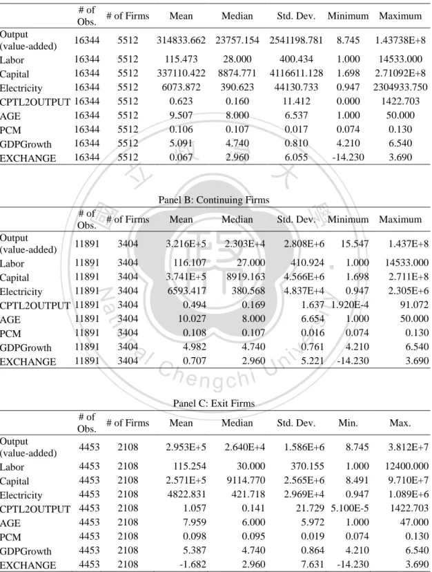
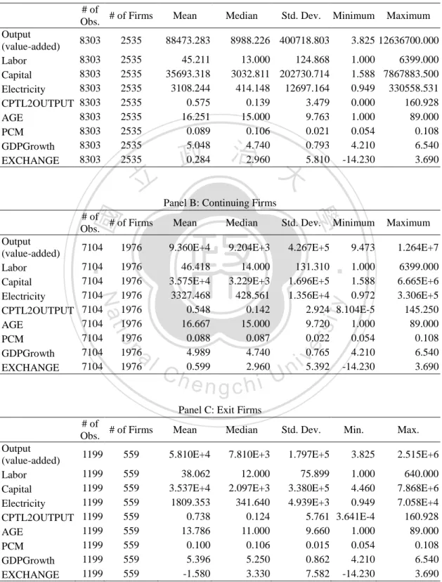
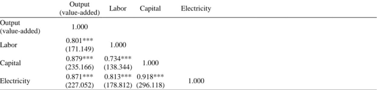
(12) List of Tables Table 1: Descriptive Statistics, Electronics Industry ................................................... 51 Table 2: Descriptive Statistics, Food Products Industry .............................................. 52 Table 3: Correlation Coefficient of Variables, Electronics Industry ............................ 53 Table 4: Correlation Coefficient of Variables, Food Products Industry ....................... 54 Table 5: Parameter Estimates of the Electronics Industry ........................................... 55. 政治大 Table 7: Average Firm-specific 立 Productivity Growth, Electronics Industry................ 57 Table 6: Parameter Estimates of the Food Products Industry ...................................... 56. ‧ 國. 學. Table 8: Average Firm-specific Productivity Growth, Food Products Industry .......... 57 Table 9: Descriptive Statistics of Technical Efficiency, Electronics Industry ............. 58. ‧. Table 10: Descriptive Statistics of Technical Efficiency, Food Products Industry ...... 58. sit. y. Nat. Table 11: The Group-specific Stochastic Frontier Estimates ....................................... 59. n. al. er. io. Table 12: The Estimates of the Industry’s Metafrontier .............................................. 60. v. Table 13: Summary Statistics of Industry Efficiency Measures .................................. 61. Ch. engchi. II. i n U.

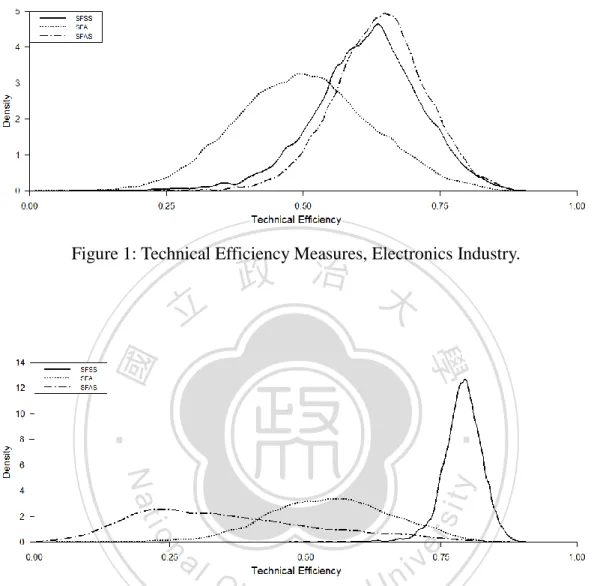
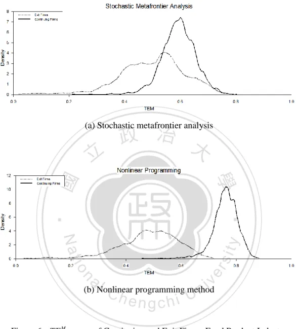
(13) List of Figure Figure 1: Technical Efficiency Measures, Electronics Industry .................................. 46 Figure 2: Technical Efficiency Measures, Food Products Industry ............................. 46 Figure 3: TGR of Continuing and Exit Firms, Electronics Industry............................ 47 Figure 4: TGR of Continuing and Exit Firms, Food Products Industry ...................... 48 Figure 5: TE M Score of Continuing and Exit Firms, Electronics Industry ............... 49. 政治大. Figure 6: TE M Score of Continuing and Exit Firms, Food Products Industry .......... 50. 立. ‧. ‧ 國. 學. n. er. io. sit. y. Nat. al. Ch. engchi. III. i n U. v.

(14) 立. 政治大. ‧. ‧ 國. 學. n. er. io. sit. y. Nat. al. Ch. engchi. IV. i n U. v.

(15) 1. Introduction Production function is a function that specifies the output of a firm for all combinations of inputs. Rather than just representing the result of economic choices, the link between output and inputs implicitly show firm’s technology, decision making, managerial ability, external shocks, and so forth. More precise estimates of production function become more relevant when we are going to investigate the firm’s characteristics.. 立. 政治大. The conventional ordinary least squares (OLS) is a useful tool to estimate the. ‧ 國. 學. parameters of a production function. Two shortcomings of the OLS are worth mentioning. The first is that it overlooks possible contemporaneous correlation. ‧. between input choices and the unobserved firm-specific productivity (Marschak and. y. Nat. Andrews (1944) and Olley and Pakes (1996) (henceforth, OP)). This simultaneity. sit. problem causes the OLS estimates to be upwardly biased when inputs are positively. n. al. er. io. correlated with productivity that has serial correlation.1 The second is that it ignores. i n U. v. the selection problem induced by endogenous exit decision. This selectivity bias. Ch. engchi. entails a downward bias in capital coefficient when a firm’s decision of exit in the next year is affected by current productivity level. This arises from the fact that the conditional expectation of productivity on current inputs and available information is decreasing in capital, as claimed by OP. Overall, the OLS procedure would overestimate labor coefficient and underestimate capital coefficient, leading to a misled measure of returns to scale. Levinsohn and Petrin (2000) note that the productivity changes are often over-predicted when adopting OLS method and the direction of productivity movement cannot be accurately captured.. 1. OP expect that the more variable the inputs, the more highly correlated with current values of productivity. Marschak and Andrews (1944) and Griliches (1957) provide detailed expositions. 1.

(16) OP proposes a semi-parametric approach to solve both simultaneity and selection problems. They suggest the use of investment, an observed variable, to proxy unobserved productivity and the use of estimated survival probabilities to correct the selectivity bias. However, many of the sample firms report zero investment due possibly to pronounced adjustment costs, which introduces the serious truncation problem. Levinsohn and Petrin (2003) (henceforth, LP) recommend the use of intermediate inputs (such as material, fuel, and electricity expenses) as the proxy to avoid the zero investment problem and thus ensure monotonicity condition of OP estimators to be held.. 政治大 the one hand, and extends立 OP/LP’s approach to include the technical efficiency of a This dissertation aims to solve both problems of simultaneity and selectivity, on. ‧ 國. 學. firm into the production frontier, on the other hand. This requires the production frontier having an extra one-sided error term, representing technical inefficiency, in. ‧. addition to unobserved productivity and idiosyncratic shocks. The emergence of the composite errors largely complicates the model. We suggest using copula methods, an. y. Nat. sit. important tool to deal with the dependence between relevant variables in the area of. n. al. er. io. finance, to derive the likelihood function that simultaneously takes the two problems. i n U. v. and composite errors into account. As far as we know, this study appears to be the first. Ch. engchi. time in the literature attempting to disentangle these topics concurrently. Based on our proposed model that solves simultaneity and selectivity in the production frontier, we attempt to compare the operating technologies of continuing and exit firms and further calculate their comparable technical efficiencies. Since the two groups of firms may operate under different technologies, the metafrontier production function model proposed by Battese et al. (2004) and O’Donnell et al. (2008) and the stochastic metafrontier model, recently proposed by Huang et al. (2012), will be adopted in this dissertation. The remainder of this dissertation is organized as follows. Chapter 2 gives a brief. 2.

(17) literature review on the simultaneity and sample selection problems. Chapter 3 develops our model that integrates the both problems under the framework of the stochastic frontier analysis (SFA). Chapter 4 introduces the stochastic metafrontier model that is able to modify the both problems. Chapter 5 describes the data source and variable definitions. Chapter 6 and 7 reports empirical results from our proposed model and the metafrontier model, respectively, while Chapter 8 concludes the dissertation.. 立. 政治大. ‧. ‧ 國. 學. n. er. io. sit. y. Nat. al. Ch. engchi. 3. i n U. v.

(18) 立. 政治大. ‧. ‧ 國. 學. n. er. io. sit. y. Nat. al. Ch. engchi. 4. i n U. v.

(19) 2. Simultaneity and Selectivity in a Production Frontier Consider a firm’s production function with Cobb-Douglas technology:. where yit. yit  0  l lit   k kit  it ,. (1). it  it  Vit ,. (2). 政治大 is plant i’s (log)output measured as value-added at time t , l 立. it. the log of. ‧ 國. 學. its labor input and kit the log of its capital input.  0 , l and  k are unknown technology parameters to be estimated. The disturbance term of  it is composed of a. ‧. firm’s productivity it and a random shock Vit . The former is a productivity index that affects the firm’s decision on input hiring and hence is correlated with the input. Nat. sit. y. choices and exit behavior. it is known to the firm and evolves over time according. n. al. er. io. to an exogenous process, but not known to researchers. The latter is an unobservable random disturbance uncontrollable by the firm.. Ch. engchi. i n U. v. Given equation (1), the OLS estimates for the two inputs are. ˆl  l .  (k , k )Cov  (l , )  Cov  (l , k )Cov  ( k , ) Cov , 2      Cov(l , l )Cov(k , k )  Cov(l , k )  . ˆk   k .  (l , l )Cov  (k , )  Cov  (l , k )Cov  (l , ) Cov . 2      Cov(l , l )Cov(k , k )  Cov(l , k )  . If the two inputs are uncorrelated with the disturbance term ( it ), i.e., Cov(k , ) . Cov(l , )  0 , the OLS estimates are unbiased. Recently, OP and LP note that the OLS estimates of labor and capital will be overestimated and underestimated, respectively,. 5.

(20) when the unobserved productivity it is, respectively, positively and negatively correlated with labor and capital. The first bias comes from simultaneity problem, arising from the fact that input choice of labor is responsible to the firm’s beliefs about it . More labor is expected to be hired in response to a higher value of current productivity it , i.e., Cov(l , )  0 , leading to an upward bias in the labor coefficient. The second bias stems from self-selection when a firm’s decision on exit is affected by its productivity. Specifically, firms accumulating larger capital stocks can expect to earn more future profits for any given level of current productivity. These firms will keep running at lower  realizations. Thus, the self-selection. 治政 inputs, survival, and all available information at t  1大 will be decreasing in capital, 立 i.e, Cov(k , )  0 , which results in a downward bias in the capital coefficient.. induced by exit decision implies that the conditional expectation of  on current. ‧ 國. 學. There are three conventional approaches to resolve the simultaneity problem,. ‧. namely, instrumental variables (IV), generalized method of moments (GMM), and fixed effects model. The first approach of the IV requires researchers to collect extra. y. Nat. sit. variables that are (highly) correlated with the explanatory (endogenous) variables and. n. al. er. io. uncorrelated with the disturbance term. IV estimators can be shown to be consistent,. i n U. v. provided the instruments satisfy the above requirements. The economics of. Ch. engchi. production theory suggests that input prices may be valid instruments because they are market-determined and directly influence the choices of inputs, but not directly enter the production function. However, input prices are often not reported by firms or cannot be recovered from their accounting data. Even though input prices are sometimes available, they may not be determined by the demand and the supply in a perfectly competitive market. It is well-known that the product price in an imperfectly competitive market is itself a function of the quantities sold. This invalidates the use of input prices as valid instruments. Even worse, the use of the IV approach is unable to solve the selectivity problem, arising from a firm’s non-random behavior of exit. The second possible solution to the simultaneity problem is the adoption of the 6.

(21) GMM technique, developed by Blundell and Bond (1998). They extend the standard first difference GMM estimation of Arellano and Bond (1991) to include additional moment conditions formed by the lagged difference of the explanatory variables that are treated as extra instruments. This approach shares the same drawback as the IV approach, i.e., it leaves the self-selection problem intact. As for the last approach, when panel data are available, the use of fixed effects model is able to solve the simultaneity problem (Hoch, 1962; Mundlak, 1961; Harrison, 1994). To correct for the simultaneity problem, the fixed effects estimation assumes that the unobserved firm-specific productivity is time-invariant. Thus,. 政治大 first difference estimation.立 An additional advantage of this approach lies in its consistent parameter estimates can be obtained by using either the within-group or. ‧ 國. 學. capability of at least partially solving the selectivity, if exit decisions are determined by the time invariant unobserved firm-specific productivity. Unfortunately, the. ‧. time-invariant assumption is strong and invalid particularly for long panel data and for data containing major environmental changes, e.g., deregulation, trade liberalization,. y. Nat. n. al. er. io. 2.1 OP/LP Approach. sit. technical change, etc.. Ch. engchi. OP propose a novel technique to handle both. iv n problems U. of simultaneity and. self-selection in the context of production function. They recommend using investment to control for the correlation between input variables and it and estimating the probit model to account for a firm’s exit decision. Later, LP argue for the use of intermediate inputs, such as materials, fuel, and electricity, to control for simultaneity, instead of investment, since in some datasets the number of observations with zero values of investment is large, which reduces the sample size considerably. We now briefly describe the estimation algorithm of OP/LP. Differing from OP, LP specifies electricity input eit as a function of kit and. it , i.e., eit  eit (it , kit ) that is strictly increasing in it . This monotonicity 7.

(22) condition ensures the following inverse function of the unobserved productivity it to be held, i.e.,. it  eit1 (kit , eit )  hit (kit , eit ).. (3). Substituting equations (2) and (3) into (1) yields a partially linear regression equation:. yit  l lit  it (kit , eit )  Vit ,. (4). it (kit , eit )  0   k kit  hit (kit , eit ) .. (5). where. 政治大. The estimation procedure is divided into two steps. In the first step, one. 立. approximates it () with a fourth order polynomial series in capital and electricity. ‧ 國. 學. and then estimate equation (4) by OLS procedure or approximates it () using kernel estimation method of Robinson (1988). The coefficient estimate of labor, ˆl , is. ‧. consistent since the series expansions or kernel estimator of it () controls for the. y. sit. io. er. assumption.. Nat. unobserved productivity and the error term of Vit is uncorrelated with inputs by. In the second step, one attempts to identify  k and correct selectivity bias. The. n. al. Ch. i n U. v. identification of  k requires separating the effect of capital on electricity function. engchi. h(·) from the effect of capital on output. Moreover, to consider a firm’s exit decision in its production function, we need additional information on a firm’s decision of liquidation. OP/LP use estimates of hît 1 ( ît 1   k kit 1 ) and predicted survival probabilities Pît to respectively control for simultaneity and selectivity biases. The bias term, g ( Pit , hit 1 ) say, arising from both simultaneity and selectivity, can thus be approximated by the fourth order polynomial series in ( Pît , hît 1 ) . The proposed regression equation is expressed as:. yit  ˆl lit   k kit  g ( Pît , hît 1 )  it  Vit 4 m 4.   k kit     mj Pîtj hîtm1  it  Vit , j 0 m 0. 8. (6).

(23) where the innovation  it (  it  E[it | it 1 , I it  1] ) and Vit are uncorrelated with. kit . 2 We can estimate (6) using nonlinear least square method to obtain the consistent estimate of  k .. 立. 政治大. ‧. ‧ 國. 學. n. er. io. sit. y. Nat. al. 2. Ch. engchi. i n U. v. Indicator variable I it  1 if the firm continues to operate and I it  0 otherwise. 9.


(25) 3. Stochastic Frontier Model with Simultaneity and Selectivity This chapter intends to develop a new approach that solves simultaneity and self-selection problems under the framework of stochastic frontier approach, in which the error term of  it in (2) contains an extra terms of a one-sided error, uit , that. 政治大 of model. Differing from. reflects technical inefficiency of the firm. We believe that this is the first time term. 立. uit entering the OP/LP type. it that captures the. ‧ 國. 學. unobserved evolution of firm-level productivity, technical inefficiency uit is exploited to represent managerial inabilities of a firm in the production process, which. ‧. is assumed to be independent of Vit and it , and uncorrelated with inputs. This allows us to generalize the OP/LP model to a stochastic frontier setting, dated back to. y. Nat. sit. Aigner et al. (1977) and Meeusen and van den Broeck (1977). We therefore refer our. n. al. er. io. model as the stochastic frontier model with simultaneity and selection (SFSS). The SFSS is specified as:. Ch. engchi. i n U. v.    l lit   k kit  it  Vit  uit , if I it  1; yit   0 otherwise, 0,. (7). I it  1 γz it  it 1 (kit 1 , eit 1 )  it  0.. (8). Equation (7) is a two-input production frontier that incorporates a productivity index. it , a technical inefficiency term uit , and a random shock Vit . uit is assumed to be a half normal random variable with a mean of zero and a constant variance, i.e.,. uit ~ iid N (0,  u2 ) ;3 Vit is assumed to be a two-sided error with a mean of zero and a 3. Term uit can also be assumed to be distributed as truncated normal, exponential, or gamma. Since all of the four distributions result in similar efficiency scores, Ritter and Simar (1997) argue for the use of a relatively simple distribution, such as half normal or exponential, rather than a more complicated 11.

(26) constant variance, i.e., Vit ~ iid N (0,  V2 ) . Variables it , uit and Vit are assumed to be mutually independent. We define the indicator function of I it  1 for the ith firm at time t if the firm continues to operate and I it  0 if the firm exits the market. We specify the survival probability to be dependent of some threshold value of productivity, it 1 , which is a function of kit 1 and eit 1 , 4 and z it , a vector of covariates that influences the exit decision of a firm. The disturbance term of it is conventionally assumed to be a standard normal random variable, making equation (8) a probit model. Following OP/LP, equations (7) and (8) lead to the estimation of the production frontier of continuing firms after solving for the problems of simultaneity. 治政 chapter, where the metafrontier model is introduced. 大立. and selection. The production frontier of exit firms will be considered in the next. ‧ 國. 學. 3.1 Controlling for Simultaneity and Selectivity. Equations (7) and (8) involve the stochastic frontier, unobserved productivity, and. ‧. limited-dependent variable concepts. To estimate the SFSS, conventional stochastic. sit. y. Nat. frontier algorithm is not directly applicable since it does not allow for the presence of unobserved productivity and exit decision. Also, Heckman’s (1979) two-step. io. n. al. er. estimation procedure cannot be employed due to the existence of it and uit . Both. Ch. i n U. v. (7) and (8) are better to be estimated jointly to yield efficient and consistent estimators.. engchi. Recently, Lai et al. (2009) propose a new approach that considers the sample selection problem in the context of a stochastic frontier model using copula functions. Copula methods is useful to capture the dependence between (7) and (8), provided it has been appropriately dealt with. Following the idea of OP/LP, we specify electricity eit as a function of it and kit , i.e., eit  eit (it , kit ). Under the condition of monotonicity the function can be. inverted to be it  hit (kit , eit ) as shown in (3). The production frontier of (7). distribution, such as truncated normal or gamma. 4 OP argues that a firm will choose to stay in the market if its productivity is greater than the threshold of it 1 . Thus, we include it 1 (kit 1 , eit 1 ) in the selection equation. 12.

(27) becomes. yit  l lit  it (kit , eit )  Vit  uit ,. (9). it (kit , eit )  0   k kit  hit (kit , eit ).. (10). where. Similar to Fan et al. (1996), equation (9) is a semi-parametric stochastic frontier model, where the functional form of hit () is unknown. Rearranging (9), we get yit  l lit  it (kit , eit )  Vit   uit    ,. 政治大立 (k , e )   (k , e )  ,. where. it. it. it. it. it. (12). it.   E  uit  . 2. . u.. ‧. ‧ 國. 學. and. (11). Nat. sit. y. Equations (11) and (12) are alike to equation (17) of Fan et al. (1996).. er. io. Pseudo-maximum likelihood algorithm listed in equations (10)-(15) of Fan et al. (1996) can be applied to obtain consistent estimates of labor, ˆl , and predicted values. n. al. Ch. i n U. v. of ît ( ît  ˆ ). Then, following the second step of OP/LP (shown in (6)), the. engchi. simultaneity bias can be approximated by powers of hît 1 ( ît 1   k kit 1 ) : 4. yit*   k kit    m hîtm1  vit  uit ,. (13). m 0. where yit*  yit  ˆl lit and vit ( it  Vit ) is assumed to be distributed as N (0,  v2 ) . The error term of vit  uit in (13) is no longer correlated with capital and hence solving the simultaneity bias problem, while the selection problem is yet to be solved. Equation (8) is used to account for a firm’s decision on exit or stay. Following OP, we use the fourth order polynomial expansion in (kit 1 , eit 1 ) to approximate. it 1 (kit 1 , eit 1 ) in the selection regression. Finally, the SFSS model becomes 13.

(28) 4  m   k kit    m hît 1   it , if I it  1; y  m 0 0, otherwise, . (14). I it  1αw it  it  0 ,. (15). * it. where  it  vit  uit and 4 m 4. αw it  γz it    mj kitj1eitm1. j 0 m 0. The composed error  it in (14) and it in (15) are here assumed to be correlated. The difficulty one is now facing is how to jointly estimate (14) and (15), in which the. 政治大. core issue is how to derive the joint distribution of the composed error  it and it .. 立. 3.2 Estimation Procedure Using Copula Methods. ‧ 國. 學. Let F () and F () be the marginal cumulative distribution functions (cdf) of  it. ‧. and it , and f () and f () are corresponding probability density functions (pdf). Define β  (  k ,  0 ,,  4 ),   ( u2   v2 )1/2 , and    u /  v . Following Lai et al.. y. Nat. sit. (2009) who utilize the Gaussian copula function to model the dependency between the. n. al. er. io. production frontier and selection equation, the log likelihood function of (14) and (15) using the entire sample can be expressed as. Ch. engchi. i n U. v. (1  I it )  ln Pr( I it  0 | w it ; α)  N T   ln f | yit* kit , ît 1 , w it , I it  1; β, α,  ,  ,  ln L(β, α,  ,  ,  )    i 1 t 1   I it    ln Pr( I it  1| w it ; α ) . . .     ,   . (16). where. f |. .   αw it    1 ( F ( it ))        f   it  1    2    1    yit* kit , ît 1 , w it , I it  1; β, α,  ,  ,   , Pr( I it  1| w it ; α) (17). . f ( it ) . 2   it     14.    it    ,    . (18).

(29) Pr( I it  0 | w it ; α)    αw it  ,. Pr( I it  1| w it ; α)    αw it  ,.  () and () denote standard normal pdf and cdf, respectively, and  is the coefficient dependence between F () and F () . Note that the conditional density function of f | () in (17) is derived based on the Gaussian copula function that describes the dependence between F () and F () . Appendix A gives detailed derivation of (16) and (17). Unfortunately, the objective function given in (16) is rather complicated and. 政治大 (2009) alternatively propose a simpler two-step estimation procedure. The first step 立 aims to estimate (15) by the standard probit model, using the entire sample, to get the. 學. ‧ 國. difficult to be estimated when the number of unknown parameters is large. Lai et al.. estimates of α . The objective function is expressed as N. T. α. ‧. max ln L1 (α)   (1  I it ) ln Pr( I t  0 | w it ; α)   I it ln Pr( I it  1| w it ; α) . (19) i 1 t 1. y. Nat. sit. Given the estimates of α , αˆ say, one can estimate the remaining parameters. n. al. er. io. (β,  ,  ,  ) using the subsample that satisfy I it  1. The objective function in the second step is formulated as. Ch. engchi. ln L2  β,  ,  ,  | I it  1 and αˆ . max. β ,  , ,  N. T. . i n U. v. .   ln f | kit , ît 1 , w it , I it  1; β,  ,  ,  , αˆ  ln Pr  I it  1| w it ; αˆ   .   i 1 t 1. (20). A final problem remains to be resolved when maximizing either (16) or (20). That is, there does not exist a closed form of F () in (17), i.e.,. F ( it ) .  it. . f ( ) d  ,. (21). . since f ( ) has no close form as shown by (18). Tsay et al. (2013) recently develop a method of approximation to (21), which relies on the use of the error function and 15.

(30) neither relies on simulation methods like Greene (2009) nor on Gaussian quadrature like Tsionas and Papadogonas (2006). This study chooses to apply the approximation approach of Tsay et al. (2013) to deduce F ( it ). Appendix B gives the detailed derivation. After getting the parameter estimates of the SFSS model, we follow Jondrow et al. (1982) to calculate technical efficiency score:. . TEit  E e  uit |  it . 立.  1 2. .   it    it /      .    it /     . (22). 政治大. ‧. ‧ 國. 學. n. er. io. sit. y. Nat. al. Ch. engchi. 16. i n U. v.

(31) 4. Switching Production Function and Metafrontier Analysis This chapter is devoted to estimate and compare the technical efficiency of different groups, i.e., exit and continuing firms, that are potentially operating under different technologies. One could first estimate a common frontier by pooling all the data of the various groups and compute and compare technical efficiencies (TEs) for the groups. 政治大 group-specific frontiers. It立 would also lack good reason if one simply estimates the. of firms. However, the so-derived common frontier may not necessarily envelop the. ‧ 國. 學. individual group-specific frontiers and compares the TEs among groups, because these TE scores are measured relative to distinct production frontiers. A metafrontier. ‧. production function model, proposed by Battese et al. (2004) and O’Donnell et al. (2008), is able to envelop group frontiers by imposing appropriate restrictions. They. y. Nat. sit. suggest a two-step procedure for estimating the metafrontier, which utilizes the SFA. n. al. er. io. in the first step to estimate the group-specific frontier and the mathematical. i n U. v. programming techniques in the second-step to estimate the deterministic metafrontier.. Ch. engchi. However, their second-step estimates from mathematical programming suffer from no statistical properties and the estimation results tend to be confounded with idiosyncratic shocks. We instead apply the stochastic metafrontier approach, developed by Huang et al. (2012), to obtain the parameter estimates of the metafrontier, which preserves statistical properties and free from the impacts of shocks. Recall that the production frontiers of exit and stay firms should be described by two distinct regression equations. Before conducting a metafrontier analysis, we use a switching regression approach that allows for correcting endogenous liquidation decision and simultaneity in such a way as to estimate group-specific production 17.

(32) frontiers consistently.. 4.1 Switching Production Frontiers Based on the SFSS model, we are able to estimate the group-specific frontiers where both endogenous liquidation decision and simultaneity are considered. For continuing firms, the model is the same as equations (7) and (8), and repeated as follows:    1l l1it  1k k1it  1it  V1it  u1it , if I it  1; y1it   10 otherwise, 0,. I it  1 γz it  it 1 (kit 1 , eit 1 )  it  0.. 政治大. As for exit firms, the model is similar to continuing firms’, but the indicator function. 立. has to be changed into I it  0 , i.e.,. I it  1 γz it  it 1 (kit 1 , eit 1 )  it  0.. (24). Nat. y. ‧. ‧ 國. (23). 學.     0l l0it   0 k k0it  0it  V0it  u0it , if I it  0; y0it   00 otherwise, 0,. sit. The above two cases explicitly consider the endogenous decision on whether exiting. n. al. er. io. or staying at the market through the indicator function. Their production frontiers can. i n U. v. be jointly estimated, which leads to consistent and asymptotically efficient estimates. Following. the. Ch. estimation. i ealgorithm n g c hdescribed. in. Chapter. 3,. the. simultaneity-corrected production frontiers are specified as: 4. y   jk k jit    jm hˆ mjit 1  v jit  u jit , * jit. (25). m 0. where hˆ jit 1 ( ˆjit 1   jk k jit 1 ) , j  0 corresponds to exit firms, and j  1 stay firms.. 4.2 Metafrontier Analysis Here we first briefly address the metafrontier production function proposed by Battese. 18.

(33) et al. (2004). For simplicity, the production frontier with unobserved productivity and is re-written as: 4. y jit   jl l jit   jk k jit    jm hˆ mjit 1  v jit  u jit m 0. (26).  ln f j (x jit , b j )   jit Here  jit  v jit  u jit , ln f j (x jit , b j ) is the logarithm of a production function, x jit a vector of explanatory variables, and b j  (  jl ,  jk ,  j 0 , ,  j 4 ) the unknown parameters corresponding to x jit . The deterministic metafrontier production function f M (x jit , b M ) that envelops all individual group’s frontiers f j is expressed as:. 政治 , 大j, i, t. f j (x jit , b j )  f M (x jit , b M )e. 立. or, equivalently,. u M jit. ‧ 國. 學. ln f j (x jit , b j )  ln f M (x jit , b M )  u Mjit , j , i, t. (27). ‧. sit. io. f M (xit , b M )  f j (x jit , b j ), j  0,1. er. Nat. that. y. where b M signifies the parameters of the metafrontier function and u Mjit  0 implies. al. n. v i n Following Battese et al. (2004),C the technology gap ratio h e n g c h i U (TGR) is defined as: TGR jit . f j (x jit , b j ) M. f M ( x it , b ).  exp(u Mjit )  1. (28). and the technical efficiency relative to the meta-frontier TE Mjit is formulated as: TE Mjit  TE jit  TGR jit .. (29). Battese et al. (2004) suggest estimating b M by mathematical programming techniques, i.e., linear or quadratic programming. Since equation (26) is a nonlinear regression model, a nonlinear programming (NP) technique is required to solve the following problem:. 19.

(34) 1. N. T. min L   u M b. 1. M jit. j  0 i 1 t 1. N. T.   ln f M (xit , b M )  ln fˆj (x jit , bˆ j ) j  0 i 1 t 1. (30). s.t ln f M (xit , b M )  ln fˆj (x jit , bˆ j ). We thus use the GAUSS module of Constrained Optimization to solve nonlinear optimization problem of (30) and obtain b M  ( lM ,  kM , 0M , ,  4M ) . As mentioned above, estimates from mathematical programming are lack of statistical properties and apt to be contaminated with statistical noises. Huang et al. (2012) recently propose a new two-step stochastic approach to estimate the stochastic metafrontier. Both Huang et al. (2012) and Battese et al. (2004) share the same first. 政治大 Huang et al. (2012) is constructed on the basis of the stochastic frontier, rather than in 立. step. Their main difference comes from the second step, i.e., the metafrontier of. ‧ 國. 學. the deterministic setting. We now turn to the second step of the new approach. Given the first step SFSS estimates of the group-specific frontiers fˆj (x jit , bˆ j ) ,. ‧. j  0, 1 , for (26), the estimation error of the group-specific frontier is calculated as: (31). io. sit. y. Nat. ln fˆj (x jit , bˆ j )  ln f j (x jit , b j )   jit  ˆ jit  v Mjit .. n. af l(x. er. The metafrontier frontier of (27) can be re-formulated by replacing the unobserved group-specific frontiers. j. Ch jit. i n U. v. , b j ) on the left-hand side with its estimated. engchi. counterpart, fˆj (x jit , bˆ j ) , from (31), i.e.,. ln fˆj ( x jit , bˆ j )  ln f M (x jit , b M )  v Mjit  u Mjit .. (32). Equation (32) turns out to be a standard SFA with v Mjit  u Mjit being the composed error term. Parameter vector b M can be estimated by the ML. Since this procedure resembles the conventional SFA, it is referred to as the stochastic metafronteir (SMF) regression. Since v Mjit involves residual ˆ jit , the variance of the disturbance term in (32) is heteroskedastic. This leads the estimated covariance matrix of the parameters to be inconsistent. This problem can be solved by relying on the use of the “sandwich” estimator for the covariance matrix. See, for example, White (1982). 20.

(35) The SMF allows for the estimated group-specific frontier in excess of the metafrontier, i.e., fˆj (x jit , bˆ j )  f M (x jit , b M ) , due to the existence of the estimation error of v Mjit . However, the metafrontier is always higher than the group-specific frontier, i.e., f j (x jit , b j )  f M (x jit , b M ) . The TGR must always be less than or equal to unity and is defined as:. . TGR*jit  E e. u M jit. . |  Mjit  1 ,. (33). where  Mjit  ln fˆj (x jit , bˆ j )  ln f M (x jit , b M ) .. 立. 政治大. ‧. ‧ 國. 學. n. er. io. sit. y. Nat. al. Ch. engchi. 21. i n U. v.


(37) 5. Data Description The primary source of data is the plant-level annually surveyed data of Taiwanese manufacturing industry, spanning 1997 to 2000 and 2002 to 2005.5 The survey is called the Industry, Commerce, and Service Census (ICSC) conducted by the Directorate General of Budget, Accounting and Statistics (DGBAS) of Taiwan. Among the 23 two-digit industries, we select two of them, i.e., electrical machinery. 政治大. and electronics industry, and food products industry as our targets. The former is. 立. known as a high-tech and highly capital-intensive industry with swift technological. ‧ 國. 學. advance, while the latter is characterized as a traditional industry and carries the opposite traits of the former.. ‧. We define the output variable ( y ) in the production function as the value-added. sit. y. Nat. that is equal to the sales revenue minus the sum of expenses on raw materials and. io. er. electricity. The capital input ( k ) is defined as the net amounts of operating fixed. al. assets. The labor input ( l ) is measured as the number of employee. The electricity. n. v i n expenses ( e ) is identified as theCintermediate input. Note that all of the dollar-valued hengchi U variables are deflated by Taiwan’s consumer price index (CPI) with the base year of 2006 and all variables are further transformed by taking the natural logarithm. The dummy variable I it  1 if firm i stays in the market; I it  0 , otherwise. The. determinants of exit used in this study are classified into three parts. The first is the threshold of unobserved productivity it 1 that is a function of kit 1 and eit 1 . Following OP, it 1 is substituted by the fourth order polynomial series expansion in (kit 1 , eit 1 ) . The second consists of a set of macroeconomic variables such as. EXCHANGEt (annual percentage change in the exchange rate of New Taiwan’s 5. The survey is not conducted in 2001. 23.

(38) Dollar versus the US dollar) and GDPGrowth t (GDP growth rate at time t ). The former intends to examine whether a depreciation or appreciation in domestic currency influence the probability of exit, while the latter wants to examine whether the macroeconomic condition affect firms’ current decision on exit. Variable. GDPGrowth t from. EXCHANGEt is taken from Taiwan Economic Journal and. Quarterly National Economic Trends published by the DGBAS. The third type of determinants are firm-/industry-specific variables. Variable CPTL2OUTPUTit is calculated as the ratio of capital to output, representing a firm’s sunk cost; AGE it signifies the age of a firm; PCM t is computed as sales revenue minus costs and. 政治大. divided by the sales revenue, which evaluates the profitability of the industry as a whole.. 立. ‧ 國. 學. [Table 1 and Table 2 here]. Tables 1 and 2 respectively report descriptive statistics of the variables for the. ‧. both industries. Each table is divided into three panels, i.e., the entire sample,. sit. y. Nat. continuing plants, and exit plants. After removing missing data and extreme values,. io. er. the sample of electrical machinery and electronics industry consists of 5,512 plants. Among them, 3,404 plants are classified as continuing plants with a total of 11,891. n. al. Ch. i n U. v. plant-year observations and the rest of 2,108 plants belong to exit firms with a total of. engchi. 4,453 plant-year observations. Food products industry consists of 1,976 continuing plants with a total of 7,104 plant-year observations and 559 exit plants with a total of 1,199 plant-year observations. As far as the whole sample is concerned, the mean values of y , l , k , and e in both industries are much larger than their medians, reflecting the distributions of these variables are skewed to the right. This implies that most of Taiwanese electronic and food products plants are small and medium enterprises (SMEs). The exit rate of electronics industry is 38.24% that is much higher than that of food product industry (22.05%). This is because the electronics industry is facing a highly uncertain. 24.

(39) atmosphere and keen competition relative to the food products industry. According to the indices of PCM and CPT2OUTPUT, the electronics industry is more profitable than the food products industry, but the former incurs higher initial sunk costs than the latter. The continuing plants are inclined to be larger than the exit ones, as the former has higher average values of output and inputs than the latter. This indicates that smaller plants tend to have higher probability of leaving the market. In addition, plants with greater sunk costs (CPT2OUTPUT) have higher probability of exiting the market in both industries.. 立. 政治大. [Table 3 and Table 4 here]. Tables 3 and 4 summarize the correlation coefficient matrices of all variables for. ‧ 國. 學. the two industries. Panel (A) reports correlation coefficients for variables in the production function and Panel (B) for variables in the selection equation. These tables. ‧. reveal that all of the variables in the production function are significantly and. Nat. sit. y. positively correlated with each other. The magnitudes of the correlation coefficients in. er. io. the selection equation are relatively smaller and their signs vary substantially. It is. al. v i n C hthe reverse is trueUin the food products industry, in the electronics industry, while engchi n. noteworthy that the correlation coefficient between EXCHANGE and PCM is positive. implying that the electronics (food products) firms can earn higher profit from the depreciation (appreciation) of domestic currency. This may be attributed to the fact that most of the electronics firms in Taiwan devote themselves to export their products and the depreciation of New Taiwan’s dollar stimulates their sales revenue.. 25.


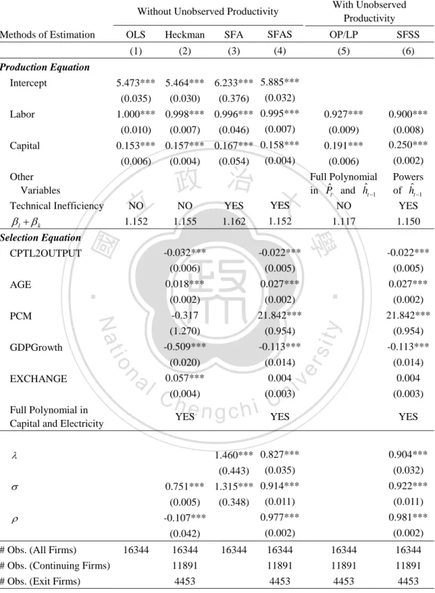
(41) 6. Empirical Results of the SFSS Model Tables 5 and 6 present parameter estimates of the production and selection equations for the two chosen industries. Columns 1-4 of the upper panel, respectively, list estimates of OLS, Heckman’s sample selection model, the conventional SFA, and the. 政治大 take the simultaneity problem into account, since the unobserved productivity  立. SFA with sample selection (SFAS) of Lai et al. (2009).6 These four models do not is. precluded from the production function. Columns 5-6 of the upper panel summarize. ‧ 國. 學. estimates of OP/LP and our proposed SFSS model, respectively. The latter two. ‧. models consider both simultaneity and selection problems, but the SFSS further generalizes the OP/LP model to a stochastic frontier framework.. er. io. sit. y. Nat. [Table 5 and Table 6 here]. al. The OLS estimates of labor and capital are 1.000 (1.081) and 0.153 (0.170) for. n. v i n C h industry. TheUsum of the two coefficients is the case of electronics (food products) engchi. equal to 1.153 (1.251), suggesting that these plants in both industries are operating under technology of increasing returns to scale. The coefficient of labor is found to be more than six times as large as that of capital in both industries. One may suspect that labor coefficient is inclined to be overestimated, while capital coefficient 6. Lai et al. (2009) combine the conventional SFA with the sample selection. Their model can be specified as:.    l lit   k kit  vit  uit , if I it  1; yit   0 otherwise, 0, I it  1αwit  it  0. The estimation procedure is similar to (16). Note that their model ignores the simultaneity problem. 27.

(42) underestimated. This is ascribable to the failure of the OLS to modify both simultaneity and selectivity problems, where the former problem entails an upward bias in the labor coefficient and a downward bias in the capital coefficient and the latter problem incurs a downward bias in the capital coefficient, as pointed out by OP. Column 2 gives the corrected estimates from the Heckman’s (1979) sample selection model. Estimated  that describes the correlation between unobserved determinants of propensity to exit the market it and unobserved determinants of output vit for electronics (food products) industry is statistically significant, suggesting that the unobservables (i.e., I it  0 ) is correlated with one another (i.e.,. 政治大 production non-randomly and 立 hence affects its production process. Compared to the. I it  1 ). The correlation further implies the firm’s liquidation decision affects its. ‧ 國. 學. OLS estimates, the coefficient of labor is slightly decreased, but the coefficient of capital is slightly increased in both industries.. ‧. Columns 3 and 4 include an extra non-negative random variable u ,. y. Nat. representing technical inefficiency, in the production function, while the unobserved. io. sit. productivity it is still excluded from the two models. Column 3 corresponds to the. n. al. er. conventional SFA and Column 4 is the SFAS model that considers a firm’s liquidation. Ch. i n U. v. decision. Differing from the OLS and the Heckman’s approach, attributing all. engchi. deviations from the production frontier to noise (e.g., measurement error, random shocks, etc.), the stochastic frontier framework assigns all deviations to both noise and inefficiency. For the case of electronics (food products) industry, the estimated labor coefficient of the SFA is slightly decreased, but the estimated capital coefficient is somewhat increased as compared to the OLS results. Similar outcomes can be detected from the SFAS estimates. In sum, the coefficient estimates of labor and capital are, respectively, decreased and increased when technical inefficiency is included in the production function, irrespective of the liquidation decision. Aside from the foregoing four models, columns 5 and 6 present the parameter. 28.

(43) estimates of the OP/LP method and the SFSS method, respectively. Recall that both methods deal with the problems of simultaneity and selectivity, but the SFSS further deliberates technical inefficiency. To eliminate the positive bias of the labor coefficient, we reformulate the SFSS model to a semi-parametric stochastic frontier model of (11) to control for the unobserved productivity and re-estimate the production function. This leads to a consistent parameter estimate of labor. For the case of electronics (food products) industry, the labor coefficients in columns 5 and 6 are 0.927 and 0.900 (0.819 and 0.809), respectively, which are 7.30% and 10.00% (24.93% and 25.07%) lower than those of OLS.. 政治大 unobserved productivity is立 indeed able to fix the upward bias in labor coefficient at. The above results confirm that the production function considering the. ‧ 國. 學. least to some extent. In addition, the upward bias of labor coefficient in food products industry is much larger than in the electronics industry. This uncovers that firms’. ‧. decision on labor hiring in food products industry is positively and more closely related to their current productivity t than in the electronics industry. One possible. y. Nat. sit. explanation is that labor input plays a more important role in food products plants. n. al. er. io. than in electronics plants that undertake a highly capital-intensive technology.. i n U. v. We next attempt to estimate  k after correcting for selection in the production. Ch. engchi. function. OP/LP recommend the use of polynomial series expansion in hît 1 ( ît 1   k kit 1 ) and predicted survival probabilities Pît to control for both. simultaneity and selectivity. Note that our SFSS model uses powers of hît 1 to control for simultaneity in production frontier and uses selection equation to simultaneously account for firm’s decision of exit, in addition to consider potential production inefficiency. Our estimation results of the electronics industry show that the capital coefficient increases from 0.153 (OLS) to 0.191 for the OP/LP and to 0.250 for the SFSS model, indicating that the capital coefficients of the OP/LP and SFSS are, respectively, raised by 24.84% and 63.40% relative to that of OLS. This is congruent with the expectation that the presence of simultaneity and selection 29.

(44) problems is likely to predict a downward bias in coefficient of capital. Moreover, the capital coefficient of SFSS is about 30.89% higher than the OP/LP. This validates the inclusion of technical inefficiency in the production function. Likewise, both capital coefficients of OP/LP and SFSS in food products industry are greater than that of OLS and the capital coefficient of SFSS exceeds that of OP/LP. Except for the consideration of technical inefficiency, our SFSS has another exclusive feature. That is, it explicitly models production frontier and selection equation as simultaneous equations. Such a model of structural equations is better to be jointly estimated like our SFSS. Conversely, OP/LP implicitly assume production. 政治大 method to remove the selection 立 bias. Since the SFSS results in the estimated values of. function and selection equation to be uncorrelated and thus suggest using the two-step. ‧ 國. 學. the dependence being equal to 0.981 and 0.740 for the two industries, the uncorrelation assumption may not be desirable.. ‧. When both simultaneity and selectivity biases are eliminated and technical. y. Nat. inefficiency is incorporated, the ratio of labor share to capital share is reduced from. io. sit. 6.535 ( 1.000 / 0.153) to 3.600   0.900 / 0.250  for electronics industry and from. n. al. er. 6.359 ( 1.081/ 0.170) to 3.275   0.809 / 0.247  for food products industry. The. Ch. i n U. v. measure of returns to scale in electronics (food products industries) lowers from 1.152. engchi. to 1.150 (from 1.251 to 1.056). The finding of increasing returns to scale seems to be reasonable, since most of the sample plants are small- and medium-sized as pointed out in the Chapter 5 of data description. These plants are anticipated to be operating at the decreasing portion of the long-run average costs. The determinants of a plant’s liquidation are also important. The less sunk costs and the older the plants are, the more likely they choose to stay in the market. However, the former results contradict most of empirical studies, e.g., Dunne and Roberts (1991) and Fotopoulos and Spence (1998), that assert that capital requirements are barriers to exit. Moreover, a depreciation in domestic currency has. 30.

(45) positive impact on the probability of staying in the market. Feinberg (2013) argues that a current depreciation is beneficial to exporters and thus leads to an increased likelihood of staying the market. Surprisingly, the economic condition has negative effect on the probability of staying in the market. [Table 7 and Table 8 here]. 6.1 Productivity and Technical Efficiency Given the parameter estimates of the production frontier, shown in Tables 5 and 6, we can calculate the firm-specific productivity measure, which is formulated as7. 政 治大 . pit  exp yit  ˆl lit  ˆk kit .. 立. (34). Tables 7 and 8, respectively, report the average rate of firm-specific productivity. ‧ 國. 學. change (  ln pit ) for the electronics and food products industries across the years of. ‧. 1998-1999, 1999-2000, and 2003-2004, where 1998-1999 and 2003-2004 are recessionary periods and 1999-2000 is expansionary period.8. y. Nat. io. sit. First, the results show that the SFSS model in chosen industries yields lowest. n. al. er. mean rate of productivity growth, indicating that models ignoring unobserved. i n U. v. productivity (such as, OLS, Heckman, SFA, SFAS), technical inefficiency (OP/LP), or. Ch. engchi. selectivity, tend to over-predict firms’ productivity growth. These over-predictions in the first five models may be attributed to high estimated labor coefficient and low estimated capital coefficient. Second, the productivity growth of electronics industry is generally higher than that of the food products industry. Third, the productivity growth in the expansionary year is higher than in the recessionary year as what we expect. However, the food products firms always have negative productivity changes, regardless of the state of the economy.. 7. This measure is also referred to as the Solow residual. Information on the date of the expansion and contraction over business cycles is judged by the Council for economic Planning and Development (CEPD), a central government bureau of Taiwan.. 8. 31.

(46) [Table 9, Table 10, Figure 1 and Figure 2 here] Tables 9 and 10 present descriptive statistics of the TE measures for both industries. Clearly, there are significant differences in TE scores among models of SFA, SFAS and SFSS. Their average TE scores in electronics industry are 50.024%, 63.858%, and 61.470%, respectively. On the other hand, the mean TE score (standard deviation) of food products industry for the three models are 54.919% (11.762%), 35.814% (16.916%), and 78.899% (3.730%), respectively. These average TE measures of food products industry show that the TE measures from the SFA and the SFAS are respectively 43.664% and 77.970% lower than that of the SFSS. The. 政治大 severe downward bias in TE, 立especially for the food products industry. Figures 1 and. foregoing reflects that the omission of simultaneity and/or selectivity can cause a. ‧ 國. 學. 2 plot the kernel density functions of TE scores for the three frontier models and the two industries. As far as the electronic industry is concerned, the curves of the SFSS. ‧. and SFAS are close to each other, but they lie on the right of the kernel density of the SFA, since their TE estimates exceed those of the SFA very much. For the food. y. Nat. sit. products industry, the kernel density function of the TE measure from the SFSS. n. al. er. io. locates at the rightmost and the remaining two curves situate on its left-hand side.. Ch. engchi. 32. i n U. v.

(47) 7. Empirical Results of the Metafrontier Models Before comparing technical efficiency between continuing and exit firms, the sample selection bias must be considered when estimating group-specific production frontiers. In the first step, we estimate the probit model with the determinants that explain. 政治大 estimate the production frontiers of (7) and (23) for the two groups by adopting 立. plants’ liquidation decisions and, in the second step, use the predicted probabilities to. [Table 11 here]. 學. ‧ 國. algorithm introduced in Chapter 3.. ‧. Table 11 reports the estimation results of group-specific stochastic frontiers.. Nat. sit. y. Using these estimates, we can test for the null hypothesis that exit and staying plants. io. er. share the same technology. The LR test statistic is significant at the 1% level of. al. significance in both industries, and hence the null hypothesis is rejected. One is led to. n. v i n C h are operating under conclude that the two types of plants heterogeneous technologies. engchi U [Table 12 here]. Table 12 reports estimates of the metafrontier obtained by SMF and NP approaches. Except for the estimates of series expansions (  0M ,,  4M ), the magnitude or the sign of the metafrontier estimates between the two methods are only slightly different. It is also worth mentioning that the estimates of  vM are statistically significant in both industries. Note that when estimating the metafrontier using NP approach, or mathematical programming techniques suggested by Battese et al. (2004), the group-specific frontier ln f j (x jit , b j ) is replaced by its estimated values of ln fˆ j ( x jit , bˆ j ) in (30). If, in the first step, the group-specific frontier 33.

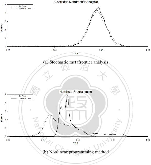
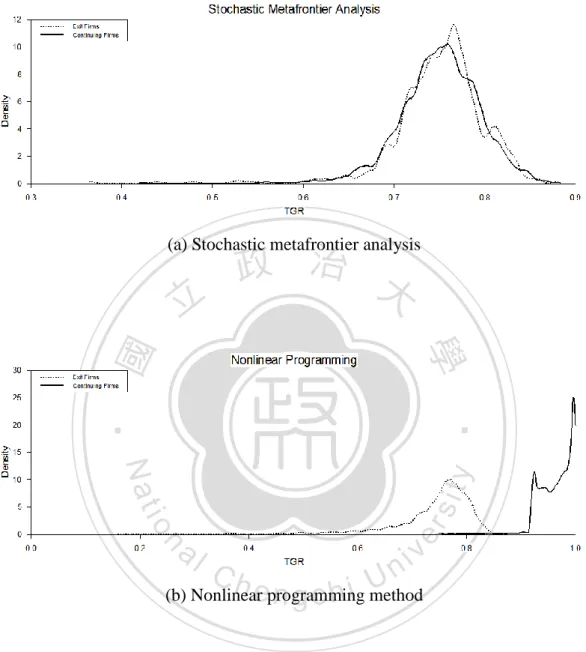
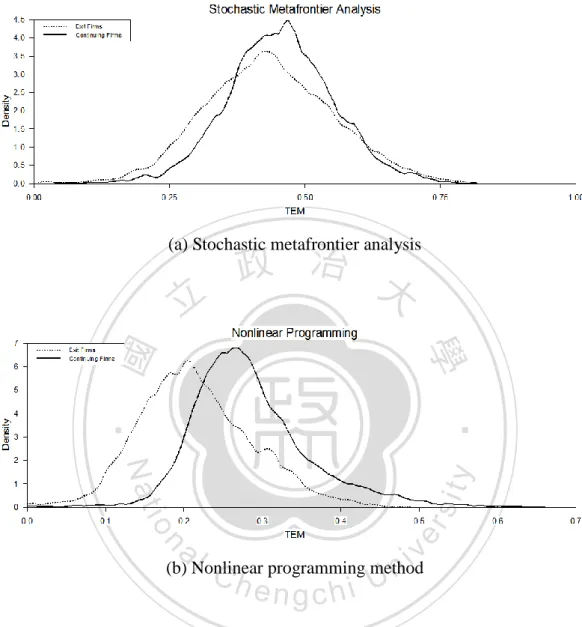
(48) estimates were perfect, i.e., ln fˆj (x jit , bˆ j )  ln f j (x jit , b j ) , the sampling error of (31) is zero and v Mjit  0 . Or, equivalently, the stochastic metafrontier specification of (32) would have  vM  0 . The significance of the estimated  vM s in both industries suggests that the NP model in the second step is potentially misspecified, since it overlooks the sampling error of v Mjit ( ln fˆj (x jit , bˆ j )  ln f j (x jit , b j )) . The SMF tends to be a preferable modeling as it allows for the inclusion of such sampling error. [Table 13 here] Table 13 reports the sample estimates of TGR, TE, and TE M for groups of exit and continuing firms. The two methods obtain quite distinct results in TGR. The. 政治大. results of NP method reveal that the continuing firms have higher average value of. 立. TGR than the exit ones, but the results of SMF uncover that the two groups have. ‧ 國. 學. similar mean value of TGR. The results suggest that, after correcting for the possible misspecification in group-specific production frontier in the first step, we find no. ‧. significant difference in the technology gap between exit and continuing firms. The. sit. y. Nat. average gaps between group frontier and metafrontier are around 27.2% and 25% of. io. n. al. er. the potential output in the two industries. [Figure 3 and Figure 4 here]. Ch. engchi. i n U. v. Conversely, the NP model draws quite a different picture. The average TGR of continuing firms are significantly higher than that of exit firms in both industries. Figures 3 and 4 further draw the kernel density functions of the estimated TGR for exits and stayers in both industries, which give similar implications to Table 13. [Figure 5 and Figure 6 here] Turning to the TE M ,. the results of SMF (NP) Table 13 reports that all firms. (continuing and exit firms altogether) in electronics industry and in food products industry can produce, on average, about 45% (26.6%) and 58.2% (72.1%) of potential output, respectively, for the SMF (NP) model, given their current input mix. In. 34.

(49) addition, the mean value of TE M of continuing firms are significantly higher than that of exit firms in both industries, suggesting that the stayers are indeed operating under a more efficient way than the exits, even though their TGR levels are alike. This implies that managerial ability plays a pivotal role on the determination of survivorship, due to the fact that the representative continuing firm has a higher TE score than the mean losers. Figures 5 and 6 display kernel density functions of TE M for both industries, which gives analogous implications.. 立. 政治大. ‧. ‧ 國. 學. n. er. io. sit. y. Nat. al. Ch. engchi. 35. i n U. v.


(51) 8. Conclusion In this dissertation, we propose a new approach to estimate a production frontier, where both simultaneity and selectivity problems are taken into accounts under the framework of the SFA. We first reformulate the production frontier as a semi-parametric stochastic regression in which the unobserved productivity is under. 政治大. control by capital and intermediate input (electricity expense). Estimating the semi-parametric model leads to consistent parameter estimate of labor. Next, we. 立. follow OP/LP’s algorithm, along with selection equation, to eliminate simultaneity. ‧ 國. 學. and selectivity biases, assuming the presence of potential technical inefficiency. In order to jointly estimate the production frontier and selection equation, we introduce. ‧. the copula function to model the dependence structure of their residuals. On the basis. sit. y. Nat. of the above framework, this dissertation further performs a metafrontier analysis to. io. er. compare the TGR and metafrontier TE between exit and continuing firms.. al. n. v i n C selectivity in the context the problems of simultaneity and h e n g c h i U of a production frontier. Some interesting results are worth mentioning. First, the SFSS model can solve. where the two problems would cause a upward bias in labor coefficient and a downward bias in capital coefficient. Second, the omission of simultaneity and sample selection, such as the conventional stochastic frontier model, is found to incur a serious downward bias in the estimate of technical efficiency. Third, the results of metafrontier analysis confirm that there is little difference in TGR between exit and continuing firms, which implies that the primary determinant on whether a firm can keep operating in the industry is its managerial ability, rather than its adoption of technology.. 37.

(52) Appendix A. Deriving the Likelihood Function of the SFSS Model. We follow the procedure of Lai et al. (2009) to derive the likelihood function of the SFSS introduced in Chapter 3. Equations (14) and (15) are repeated as follow. where. 4   k     hˆm  v  u , if Iit  1; yit*   k it m 0 m t 1 it it 0, otherwise, . (A1). I it  1αw it  it  0 ,. (A2). 政治大. yit*  yit  ˆl lit , hît 1  ît 1   k kit 1 , uit ~ N (0,  u2 ) ,. 立. vit ~ N (0,  v2 ) , and. it ~ N (0,1). For simplicity, we denote β  (  k ,  0 ,,  4 ) and the composed error. ‧ 國. 學.  it  vit  uit . Let F (·) and F (·) be the marginal cdfs of  it and it , and f (·) and f (·) their corresponding pdfs. According to the Sklar’s theorem, there exists a. ‧. unique copula function C (·) such that. y. (A3). io. sit. Nat. F  ( , )  C ( F ( ), F ()),. n. al. er. and C (·) is unique if both F (·) and F (·) are continuous. Since y. * it. Ch. in (A1) is only observed when I it. engchi. iv n  1Uin the selection regression, we. can modify (A3) to build conditional probability of  :. . F |  it | it  αw it. . . Pr     it , it  αw it  Pr  it  αw it . . Pr     it ,    Pr     it , it  αw it  1  Pr  it  αw it . . F ( it )  F    it , αw it  1  F  αw it . . F ( it )  C  F ( it ), F  αw it   1  F  αw it . 38. ,. (A4).

(53) where 1  F  αw it   Pr  it  αw it   Pr( I it  1| w it ; α).. (A5). Taking a partial derivative of (A4) with respect to  it , we get. . . f |  it | it  αw it . f ( it ) 1  C  F ( it ), F  αw it    1  F  αw it . (A6). ,. where C ()  C () / F . Since  it  yit*   k kit   m0  m hîtm1 , we can rewrite (A6) 4. as. . f ( it ) 1  C  F ( it ), F  αw it   . . f | yi*t | kit , ît 1 , w it , I it  1; β, α . 立.  αw  政治1  F 大 . .. (A7). it. According to (A5) and (A7), the maximum likelihood function based on the full. ‧ 國. T. . . ‧. N. 學. sample is. Iit. L   Pr( I it  0 | w t ; α)(1 It )  f | yit* | kit , ît 1 , w it , I it  1; β, α Pr( I it  1| w it ; α)  .   i 1 t 1. sit. y. Nat. (A8). n. al. er. io. It remains to derive the copula function of C () in (A7), in which the normal. i n U. v. copula is assumed. Let r1  F ( ) and r2  F ( ) and define  †   1 (r1 ) and. Ch. engchi.  †   1 (r2 ) such that both  † and † follow a bivariate standard normal. distributions. The joint distribution of  and  in (A3) can be written as. F   1 (r1 ), 1 (r2 ),   C (r1 , r2 ), where () denotes the standard normal distribution function. Roncalli (2002) derives the normal copula function C () as:9   1 (r )   1 ( )  2  d . C (r1 , r2 ;  )     2   1   0   r1. (A9). This allows us to obtain C () by taking the partial derivative of (A9) with respect to 9. See Cherubini et al. (2004) for more details. 39.

(54) the r1 , i.e., C .     1 ( F ( ))  C (r1 , r2 ,  )  .   2   r1 1    . (A10). The foregoing implies that, under the assumption of normal copula, the log-likelihood function given by (A8) can be written as. (1  I it )  ln Pr( I it  0 | w it ; α)   ln f | yit* kit , ît 1 , w it , I it  1; β, α,  ,  ,  ln L(β, α,  ,  ,  )      I i 1 t 1  it   ln Pr( I it  1| w it ; α ) . . T. ‧ 國. Pr( I it  1| w it ; α). ‧. f ( it ) . 學. . f | yit* kit , ît 1 , w it , I it  1; β, α,  ,  ,  . αw it    1 ( F ( it ))     f   it  1    2    1    . io. Pr( I it  0 | w it ; α)    αw it  ,. er. Nat. 2   it    it     ,       . y. 立 . .     , (A11)   . 政治大  . where. sit. N. n. a Pr( l CI  1| w ; α)    αw n. i v hengchi U it. it. it. The log-likelihood functions (A11) and (16) are the same.. 40. ,.

(55) Appendix B. The Derivation of F (Q). Let v ~ N (0,  v ) and u ~ N (0,  u ) , the probability density function of the composite error   v  u is known as:. f ( ; ,  ) . 2     .      ,   . where    u /  v . The cdf of  can be specified as. 2. F (Q) . I (Q), 政 治大. 立.   /       ( )d     Q. I (Q) .  d  . . 學. ‧ 國. where. ‧. n. engchi. erf ( )  2. sit. io and the error function. Ch. er. Nat. al. if   0; 1,  sign( )  0, if   0; 1, if   0; . y. Define a sign function as:. i n U. v. 2.   (t )dt 0.  2. . . 2  1.. Let a   /  and b  1/  . Following the derivation of Tsay et al. (2013), I (Q) can be approximated by:. 41.

(56)   ac1  2Q b 2  a 2c2  sign(Q)      I app (Q)  1  erf  2 2    2 b  a c 2       a 2 c12 1  exp  2  2 2 2   4b  4a c2  4 b  a c2.  bQ   erf  2  1  sign(Q)     , 2b 2 . where c1  1.09500814703333 and c2  0.75651138383854 .. 立. 政治大. ‧. ‧ 國. 學. n. er. io. sit. y. Nat. al. Ch. engchi. 42. i n U. v.

(57) Reference Aigner, D. J., C. A. K. Lovell, and P. Schmidt (1977) “Formulation and Estimation of Stochastic Frontier Production Function Models,” Journal of Econometrics, 6, 21-37. Arellano, M. and S. Bond. (1991) “Some Tests of Specification for Panel Data: Monte Carlo Evidence and An Application to Employment Equations,” Review of Economic Studies, 58, 277-297.. 政治大. Battese, G. E., D. S. P. Rao, and C. J. O’Donnell (2004) “Metafrontier Production. 立. Function for Estimation of Technical Efficiencies and Technology Gaps for Firms. ‧. ‧ 國. 91-103.. 學. Operating Under Different Technologies,” Journal of Productivity Analysis, 21,. Blundell, R. and S. Bond (1998) “Initial Conditions and Moment Restrictions in. sit. y. Nat. Dynamic Panel Data Models,” Journal of Econometrics, 87(1), 115-143.. n. al. er. io. Cherubini, U., E. Luciano and W. Vecchiato (2004) Copula methods in finance. John Wiley & Sons, Hoboken, NJ. Ch. engchi. i n U. v. Dunne, T. and M. Roberts (1991) Variation in Producer Turnover across US Manufacturing, in Entry and Market Contestability: An international comparison, (Eds) P. Geroski and J. Schwalbach, Blackwell, London. Fan, Y., Q. Li, and A. Weersink (1996) “Semiparametric Estimation of Stochastic Production Frontier Models,” Journal of Business and Economic Statistics, 14, 460-468. Feinberg, R. (2013) “Internation Competition and Small-firm Exit in US Manufacturing,” Eastern Economic Journal, 39, 402-414. Fotopoulos, G. and N. Spence (1998) “Entry and Exit from Manufacturing 43.

(58) Industries: Symmetry, Turbulence and Simultaneity: Some Empirical Evidence from Greek Manufacturing Industries,” Applied Economics, 30(2), 245–62. Greene, W. (2010) “A Stochastic Frontier Model with Correction for Sample Selection,” Journal of Productivity Analysis, 34, 15-24. Griliches, Z. (1957) “Specification Bias in Estimates of Production,”. Journal. of Farm Economics, 39, 8-20. Harrison, A. E. (1994) “Productivity, Imperfect Competition and Trade Reform: Theory and Evidence,” Journal of International Economics, 36, 53-73.. 政治大. Heckman J. (1979) “Sample Selection Bias as A Specification Error,”. 立. Econometrica, 47, 153–161.. ‧ 國. 學. Hoch, I. (1962) “Estimation of Production Parameters Combining Time-series and Cross-section Data,” Econometrica, 30(1), 34-53.. ‧. Huang, C. J., T.-H. Huang, and N.-H Liu (2012) “A New Approach to Estimating. y. Nat. n. al. er. io. Working Paper.. sit. the Metafrontier Production Function Based on a Stochastic Frontier Framework,”. i n U. v. Jondrow, J, K. Lovell, I Materov, and P. Schmidt (1982) “On the Estimation of. Ch. engchi. Technical Inefficiency in the Stochastic Frontier Production Function Model,” Journal of Econometrics, 19, 233-238. Lai, H.-P., S. Polachek, and H.-J. Wang (2009) “Estimation of a Stochastic Frontier Model with a Sample Selection Problem. Working Paper, Department of Economics, National Chung Cheng University, Taiwan. Levinsohn, J. and A. Petrin (2000) “When Industries Become More Productive, Do Firms? Investigating Productivity Dynamics,” NBER Working Paper 6893. Levinsohn, J. and A. Petrin (2003) “Estimating Production Functions Using Inputs to Control for Unobservables,” Review of Economic Studies, 70(2), 341–372. 44.