考量街道寧適性下步行可及性與移動性之研究

(1)

國立交通大學

運輸科技與管理學系

博士論文

考量街道寧適性下步行可及性與移動性之研究

Walking Accessibility and Mobility with the Consideration of Street

Amenities

研究生：蔡耀慶

指導教授：許巧鶯教授

(2)

考量街道寧適性下步行可及性與移動性之研究

Walking Accessibility and Mobility with the Consideration of Street

Amenities

研究生：蔡耀慶 Student：Yau-Ching Tsai

指導教授：許巧鶯 Advisor：Chaug-Ing Hsu

國立交通大學

運輸科技與管理學系

博士論文

A Thesis

Submitted to Department of Transportation Technology and Management College of Management

National Chiao Tung University in partial Fulfillment of the Requirements

for the Degree of Doctor

in

Transportation Technology and Management June 17 2013

Hsinchu, Taiwan, Republic of China

(3)

誌謝

感謝陪我走過這八年的許老師、我的家人、容瑛及研究室同仁（慧潔

學姐、剛伯學長、佳紋、憲梅、郁哲…），謝謝你們的包容與付出。感謝

指導過我的所有師長們：張新立院長、卓訓榮主任、吳水威老師、王晉元

老師、黃家耀老師…，提供行政協助的系辦助理們，以及在運輸年會一起

打拚過的學弟妺們。更要感謝四位口試委員：任維廉老師、林俊源老師、

林楨家老師以及金家禾老師，在口試時提供許多寶貴的建議。另外，我也

要謝謝交通處的所有同仁，跟你們共事是非常快樂的事。最後，感謝天主

～我終於畢業了！

(4)

I

摘要

近年來，街道改善計畫常藉由提升街道空間寧適性以提升視覺、心理愉悅度進而提升步行意願，其對行人生理機制之影響亦受到關注，特別是當今社會高度重視步行對健康之效益。行人廊道為都市中常見的線型步行空間，主要用於進出交通場站或抵達鄰近活動發生點，其規劃設計議題大多聚焦在容量設計上，然而近年研究發現平面設計型態亦會影響行人流量。再者多數已開發國家未來都須面對人口老化問題，低速度的老年行人使用大眾運輸系統比例將增加，廊道內步行移動性差異逐漸擴大，增加碰撞與局部擁擠發生機率。對此本研究分別從心理與生理量測法分析街道寧適性對步行可及性以及廊道空間平面設計對步行移動性之影響。以行人路權、夜間照明、綠美化、街道傢俱、沿途商業活動、鋪面以及水景等七個街道空間元素為主要寧適性因子，分別從心理與生理的角度探討街道寧適因子變動下對步行意願與距離之影響。心理層面同時設計顯示性與敘述性偏好問卷，調查不同起迄對步行路線選擇行為，以降低各因子共線性並提高資料變異度，校估步行效用函數，進而觀察各寧適性因子變動下對步行意願與距離之影響。生理層面則透過實驗設計，加入上述因素之影響，改善並應用 Pandolf et al.(1977) 模式於捷運旅客步行能量消耗之調查，進而從能量分布函數推導出各街道空間下之步行可及距離。為確保步行安全性與系統效率，提升民眾步行意願，本研究以 Helbing et al. (2000)模式為基礎，並透過行為觀察構建步行模式，從真實案例歸納出六種替選方案，應用 C 語言設計代理人模擬程式，探討可有效提升行人流速的平面設計手法。結果顯示綠美化與商業活動對於步行意願具有正效應，步行時間則為負效應，亦即規劃者在進行街道改善計劃時可優先從綠化與沿街商業活動著手改善；行人路權在敍述性偏好中具有極顯著的效應，但在顯示性偏好中則為不顯著，代表實際行為與假設性意願存在差異；另外，照明設計與街道傢俱手法，對於提升步行意願皆為不顯著。生理層面部分，經能量消耗實驗校估出 Pandolf et al.(1977)修正模式，應用於能量計算以求得次數統計並進行適配度檢定，結果發現步行能量消耗呈現 Gamma 分布，意謂行人於通勤旅次中普遍追求節能、省力之特性。應用花台進行中央分隔與推廣低速度行人靠兩側行走可有效提升行人流速；若應用座椅區隔出老人專用空間，雖然提高安全性卻大幅降低有效寬度，影響年輕行人之步行速度。本研究結果成果可提供規劃者從事步行可及性指標制定、街道改善方案評估以及步行行為分析之參考依據，也進一步解釋為何規劃者多傾向採用全開放式空間，但透過集體行為規範同樣可提高系統效率而又不影響廊道的有效寬度。關鍵詞：步行意願、能量消耗、顯示性及敘述性偏好、路線選擇模式、代理人模擬法。

(7)

ii

ABSTRACT

How to improve street amenities (SA) to both raise willingness to walk (WTW) and level of service (LOS) is a crucial issue for planners when designing a pedestrian-friendly environment in terms of accessibility and mobility. However, few studies have provided rigorous and systematic analysis to aid this practice.

Thus, this research addresses this issue with three topics: first, defining measures of WTW to represent variation across environments; second, estimating WTW for the varied levels of SA; third, designing the arrangement of SA to raise LOS when mobility difference is high. Attributes of street amenities are classified, such as right of way, lighting, planting etc., and WTW is defined with both physiological and psychological measure: energy expenditure (EE) and walking time. The WTW measures taking into account the effects of SA are estimated by designing energy expenditure and conducting revealed and stated route choice experiments. The Pandolf et al. (1977) model is used to analyze the walking energy expenditure (WEE). The terrain factor is adjusted using the calibrated regression function to fit the urban street space in the experiment. To avoid violation of the irrelevance of independent alternatives (IIA), random-parameters logit is applied to build route choice model. With respect to nature of pedestrians and data scale, Helbing’s (2000) agent-based model is modified to model passing behaviors. The simulations are conducted with the designed simulator at Fruin’s (1971) six levels of flow to fully represent pedestrian flow. Results show that WEE sample suggests a Gamma distribution. The accessible walking distance pattern around a service facility should be designed based on the service contour lines which take into account the effects of SA. Results of pedestrian route choice show improvement for right of way, lighting, planting, retailing, and fountains, would significantly enhance WTW. The results of ABM indicate that a corridor in which a line of round objects, such as potted plants, are positioned to divide a bidirectional stream of pedestrian traffic, can result in a relatively smoother flow than if the objects were rectangular in shape, e.g., benches. It is worth noting that by promoting collective self-organizing when it comes to walking direction, and by providing a sub-lane along the wall for slower walking, a better performance can be obtained, even without reducing the effective width.

Key words: willingness to walk, energy expenditure, revealed and stated preference, route choice experiment, agent-based model.

(8)

iii

LIST OF TABLES

Table 1 Attributes of pedestrian environment quality. ... 11

Table 2 Spatial characteristics of the experiment sites ... 20

Table 3 Summary of independent variables ... 21

Table 4 Example of O-D pair table ... 22

Table 5 Experiment outcome summary ... 25

Table 6 Results of regression analysis ... 26

Table 7 Individual and trip characteristics of the commuters ... 29

Table 8 Estimates of walking distance by street type and gender ... 31

Table 9 Attributes and levels of SA ... 36

Table 10 List of the individual characteristics and the specific constant. ... 38

Table 11 List of the designed SP alternatives. ... 40

Table 12 Estimation results for utility function. ... 42

Table 13 WTW estimation for levels of improvement ... 43

Table 14 Spatial characteristics of the alternative routes in Caogong Canal Regeneration. .... 46

Table 15 Results of chi-square test for Caogong Canal Regeneration. ... 47

Table 16 Improvement cost ranking of Caogong Canal Regeneration. ... 48

Table 17 Percentage of elderly in the pedestrian flow ... 54

Table 18 Changes of LOS as the percentage of elderly increases ... 55

Table 19 Characteristics of the six alternatives. ... 58

(9)

iv

LIST OF FIGURES

Figure 1 The concept of the traditional walking distance. ... 1

Figure 2 A real case in Hsinchu City. ... 4

Figure 3 Analytical framework ... 6

Figure 4 The trade-off between walking distance and PEQ. ... 12

Figure 5 Relationship between terrain factor and walking distance. ... 18

Figure 6 Seven WEE experiment sites ... 19

Figure 7 The statistical distribution of the observed WEEs. ... 28

Figure 8 An example of IIA violation in a pedestrian’s route choice. ... 35

Figure 9 An example of a stated preference question ... 39

Figure 10 Plot of relative scale factor and log-likelihood. ... 44

Figure 11 Caogong Canal before and after improvement. ... 45

Figure 12 The three alternative routes between Fongshan Stadium and Fongshan Station. .... 46

Figure 13 The location of 10 agents at each 10s. ... 53

Figure 14 Simulation flow. ... 56

Figure 15 Verification of our models. ... 57

Figure 16 Configuration of six types of corridor design. ... 57

Figure 17 The service area with cosideration of WEE ... 63

(10)

v

GLOSSARY OF SYMBOLS

m: body weight(kg)

 

t

v : walking speed function(m/s)

r

: position

 

r

 : friction function

g: the gravitational acceleration(m / s2)

t: a period of walking time(s)

ew: the consumed energy, the unit of ew is in joule(J)

P: the amount of street type

sp: walking distance on a type p street(m)

μp: the friction value on a type p street

W: the metabolic rate, energy expenditure per second (J/s, watts) l: the load carried(kg)

G: the grade (%)

n: the terrain factor value n

~

: the observed value of n

 

x

 : the friction function consisting of a vector of street factors that significantly affect the WEE

M : the number of factors

i

C : the choice set of pedestrian i , consisting of several alternative routes

io

U : the random utility of alternative route o for pedestrian i

io

V : the systematic utility

ε : the error term in regression function

io

 : the random component of utility function

o (o): the alternative belonging to pedestrian i ’s choice set C _i

 : the scale factor

ioq

x

: the value of street amenity q during pedestrian i 's route o

CV _{: compensating variation}

 _{: the marginal utility of walking time(s)}

i

 : the subject-specific stochastic component for each 

0

n

V : the initial state of utility

 n

V : the level of utility in the subsequent state

0 i r : the origin  i r : the destination 

(11)

vi object

ij

u : pedestrian i and j produce a potential energy (J)

i

r

: the radius of pedestrian i’s personal space (m)

ij

d : the distance between the pedestrian i and j’s center(m)

i

e : the normalized direction vector

(12)

1

CHAPTER 1 INTRODUCTION

In this chapter, I first illustrate the importance of building pedestrian-friendly environment and the issues existing in the practice. After it, the objectives are set. Then, I present the research framework to illustrate the relationship among the study subjects and the approaches I used.

1.1 Motivations and background

Reports have shown that transportation and land use change contribute a total of nearly 31.7% of the greenhouse gas emissions. These trends are increasingly quite dramatically, especially in the countries with emerging and newly developed economies such as mainland China, India and Brazil (USEPA, 2009; WRI, 2005). Walkable environment is regarded as a solution to this problem.

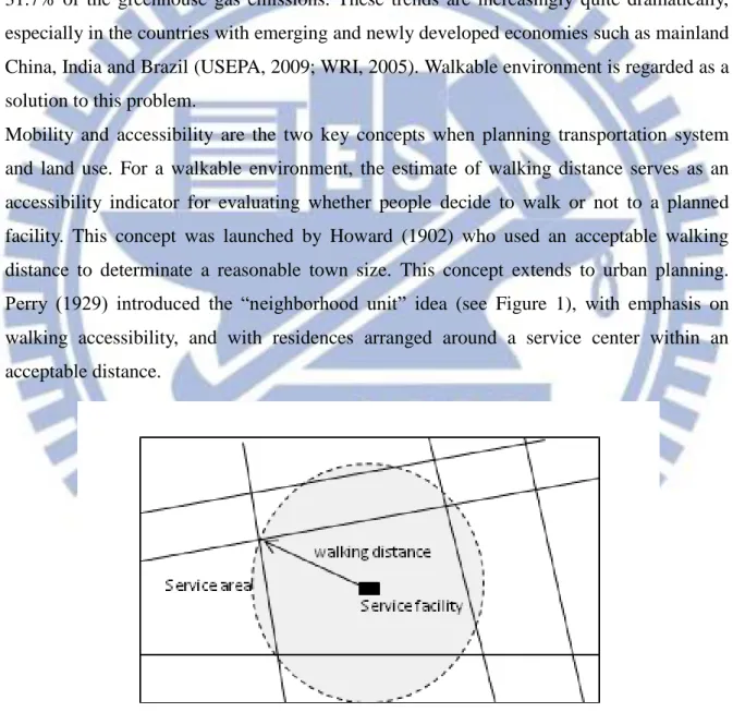
Mobility and accessibility are the two key concepts when planning transportation system and land use. For a walkable environment, the estimate of walking distance serves as an accessibility indicator for evaluating whether people decide to walk or not to a planned facility. This concept was launched by Howard (1902) who used an acceptable walking distance to determinate a reasonable town size. This concept extends to urban planning. Perry (1929) introduced the “neighborhood unit” idea (see Figure 1), with emphasis on walking accessibility, and with residences arranged around a service center within an acceptable distance.

Figure 1 The concept of the traditional walking distance.

To-date, new planning paradigms, e.g., Transit Oriented Development (TOD), New Urbanism, Compact City, continue to apply walking distance not only to create a

(13)

2

pedestrian-friendly environment but also to reduce greenhouse gas emissions by encouraging transit ridership and walking frequency (Banai, 1998; Calthorpe, 1993; Cervero and Kockelman, 1997; Cervero et al., 2009; WRI, 2005). Its application is also found in the retailing theory where it is used to estimate the number of walk-in customers and in location-allocation modeling studies where it serves as a parameter for designing the maximal covering model (Brown, 1996; Hsu and Chen, 1994; Owen and Daskin, 1998). Although the method has been and still is applied in many fields, its measure does not reflect variability. In fact, there are various measures recorded in the literature, but few studies that explore their variation. Howard (1902) initially set it as a half mile; Perry (1929) used a quarter mile (5-minute walk) as the radius of a neighborhood unit; and in Sweden it was set as a range of about 300~500m (Lynch and Hack, 1984). The characteristics of the pedestrian, e.g., trip purpose, gender, and age, and urban context may alter the acceptable distances (Clifton and Krizek, 2004). For example, Pushkarev and Zupan(1975) compared the cumulative distribution of walking distances for a trip at two Manhattan buildings. They found that trips to eat had the shortest walking distance and that shopping trips had the longest ones among five purposes (eat, work, pleasure, business and shop). However, to-date few studies have explored the variation in walking distance and its implication for pedestrians. A useful method to express the variability of walking distance is the statistical distribution. As mentioned earlier, Pushkarev and Zupan(1975) applied this method to analyze walking distances. Seneviratne (1985) observed the distribution of walking distances by conducting a survey in the central business district of Calgary, Canada. It is worth noting that Seneviratne (1985) derived the critical distance of 243m (796 ft), at the maximum rate of change of the distribution function as the more reasonable estimate for the average walking distance of 250m (819 ft). This advanced application of statistical frequency for estimating walking distance inspired our later analysis.

However, contrary to the discussion on the variation in walking distance, there is much less concern regarding the variability across pedestrian environments. People generally agree that the higher the pedestrian environment quality (PEQ) the farther, within reason, they are willing to walk, and this finding is backed up in the literature (Untermann, 1984; Zacharias, 2001). Nevertheless, few studies have explored this issue with systematic analysis. Gehl (2001) and Untermann (1984) investigated the change of frequency based on the improvement of PEQ, but they did not include any change in walking distance. Lövemark (1972) recognized the effects of PEQ on willingness to walk and claims that a pleasant

(14)

3

pedestrian environment encourages an up to 30 percent greater walking distance. To date his study is the one closest to the issue addressed here, but it still does not show any details. In urban pedestrian environment, PEQ is associated with level of street amenities (SA), e.g., right of way, lighting, planting, pavement, street furniture, retailing, and fountains (Booth, 1983; Mitra-Sarka, 1994). Since better street space would encourage people to ride transit and to walk more frequently (or for longer), street improvement projects are broadly proposed. This could include enhancing street lighting, increasing the greenbelt area, and so forth. Even their benefits have been demonstrated in many studies with reference to the appreciation of real estate value (Cheshire and Sheppard, 1995; Correll, Lillydahl and Singell, 1978); planners have recently focused on the extent to which street improvement projects have raised WTW. However, similarly, few have conducted systematic investigations to demonstrate relationship between WTW and SA. The necessary requirements are a suitable measure of WTW, an analytical model, and adequate empirical data. Street improvement studies usually evaluate the effects of a single street amenity, such as lighting (Willis, Powe, and Garrod, 2005). They tend to either focus on economic valuation without link to users’ behavioral intentions, or perform qualitative analysis, without specifically suggesting a useful planning tool.

Additionally, arrangement of SA also affects walking mobility. This can be observed in a corridor when mobility difference is very high. A substantial difference in mobility would cause uneven pedestrian flow, particularly when it is due to elderly pedestrians. The rapidly aging population, especially in the developed countries has changed the demographic profile in Taiwan, and will continue to have a drastic impact on transportation planning in the coming decade (Meyer and Miller, 2001). It will result in temporary and local congestions in high density pedestrian corridors. Consequently, commuters must spend more travel time in these corridors to bypass slow pedestrians and to avoid a collision. This type of congestion tends to happen around elderly pedestrians walking very slowly. Figure 2 shows a photograph of a local congestion being created on a street in Taiwan.

However, designing SA to raise corridor performance is rarely discussed. Unless a pedestrian corridor is a new construction, the space available for widening the corridor is extremely limited. In that situation, the improvement program should focus on space design. But, when planning a pedestrian corridor, planners must pay close attention to capacity design, because misallocation tends to be the major source of pedestrian congestion in high density areas (Pushkare and Zupan, 1975). Fruin(1971) characterized the quality of the

(15)

4

pedestrian flow at various levels of maximum capacity as level-of-service (LOS) to aid capacity design. This method is still widely used today, and its assumptions allow us to explore any new issues that we have to face, now or in the future. It assumes that a pedestrian flow is an even or homogenous stream, but in reality it is usually uneven. Pushkarev and Zupan found that a platoon of pedestrians causes an uneven flow, and they improved the traditional LOS method by taking the platoon effect into account.

Figure 2 A real case observed in Hsinchu City where an elderly man walks very slowly, and some of the surrounding younger pedestrians try to bypass while keeping a buffer zone in order to avoid collision. Some of them slowed down or stopped to give him the

right of way.

Mobility differences are also dangerous for the safety of the elderly on the streets. Although my observation showed that the young tend to give the right of way to the elderly, the potential risk for a collision to occur remains. Both the elderly and the younger generations require space arrangement not only to prevent possible conflict between the 2 groups, but also to maintain operation efficiency. This problem intensifies in and around downtown healthcare institutions. Although there are provisions for people with disability, many of the elderly I mentioned here can walk freely, but do so at low speed.

The reports of successful real-world cases can be of use in corridor design, but only a few of them performed systematic analyses which could benefit planners to rationally and broadly

(16)

5

assess their design (Marcus and Francis, 1998). Fortunately, Helbing and his partners built agent-based models (ABMs) to study pedestrians. They found that geometric form and design elements can stabilize the flow pattern and make them more fluid (Helbing et al., 2001; Helbing et al., 2000). However, their discussions don’t cover the issue addressed in this thesis.

1.2 Objectives

Thus, this research addressed the above issues in three ways: First, I aim to improve the definition of traditional walking distance by taking into account the effect of the PEQ. Based on this improvement, I could then show the various walking distances according to the values of PEQ. I introduced the concepts of willingness to walk (WTW) and walking energy expenditure (WEE) and used WEE as a physiological measurement of WTW. Pandolf et al. (1977) provided an applicable metabolic rate (energy expenditure per time) equation, and I used heart rate method to measure energy expenditure. However, the environmental factors in Pandolf et al. (1977) only involved slope and terrain, so this study developed a model to predict the adjusted terrain factor by incorporating the effect of PEQ. Second, I aim to develop models to determine which attributes of SA would psychologically raise people’s WTW and to estimate how much WTW a specific improvement would increase. Because better street space can encourage people to walk more frequently (or for longer), my analysis is based on the notion of linear correlation between SA and WTW (Cervero and Kockelman, 1997; Cervero et al., 2009; Gehl, 2001; Untermann, 1984). Then, I classified the attributes of SA into right of way, lighting, planting, pavement, street furniture, retailing, and fountains (Booth, 1983; Mitra-Sarka, 1994) to systematically represent an improvement project as systematic alternative. I denoted walking time as psychological measures of WTW, not walking distance, because it is more suited to a self-reporting survey. A higher WTW was considered as an effect of improved amenities from improvement projects and was measured by modeling pedestrians’ route choices. I believe these results can be applied to aid planners’ street improvement practices, such as project design or alternative evaluation.

Third, I aim at building an approach to explore which type of pedestrian corridor design can improve the congestions resulting from the high difference in mobility among pedestrians. This issue needs to be addressed to respond to Taiwan’s rapidly aging population. I built ABMs and designed a simulation experiment using fine-scale data to investigate the issue of the difference in mobility among pedestrians. This takes individual characteristics into

(17)

6

account and aids to planners’ street improvement practices, such as project design or alternative evaluation.

1.3 Research framework and approaches

The research framework of the thesis is shown in Figure 3:

Figure 3 Analytical framework

As stated in the above, the research subjects include mobility, accessibility and street amenities. I first introduce the relationships among them and define willingness to walk. These may not be the first mentioned, but, here, I made a rigorous statement for it. Only based on it, the following systematic analyses can be successfully conducted. In term of physiology, WTW can be measured with walking energy expenditure (WEE). PEQ can represent the quality of street amenities. But how do I find an approach that enabled us to analyze the effect of PEQ on WEE? Heart rate (HR) can be a suitable indicator, and Pandolf et al. (1977) provides an applicable metabolic rate equation. However, the environmental factors in Pandolf et al. (1977) only involve slope and terrain. Previous studies categorized

1. Attributes: sidewalk planting lighting …… 2. Arrangement

Pedestrian-Friendly Environment Planning

Accessibility Mobility Walking Distance Street Amenities Walking Speed 2 Corridor Design by Flow Characteristics WTW Variation Evaluation of Street Improvement Agent-based Simulation Energy Expenditure Route Choice: RP & SP Walking Time Physiological Measure Psychological Measure Flow Charact eristics 1

(18)

7

the values of the terrain factors based on the type of road surface. So this study developed a model to predict the adjusted terrain factor by incorporating the effect of PEQ. Statistical distribution was applied to observe the characteristics of the walking behavior and to estimate distances based on the cumulative probability levels of WEE. The level of WEE represents the level of effort expended during walking. This research assumes that the greater the effort required by the pedestrian to walk, the shorter the distance will be they are willing to walk. Thus, the distance that a certain proportion of pedestrians are willing to walk can be estimated from the cumulative probability of WEE.

Secondly, I introduce a psychological measure of WTW: walking time to meet the requirement when modeling pedestrians’ route choices. Route choice commonly exists in people’s daily walking trips, and has been applied to study pedestrian behavior, such as walking trajectory (Antonini et al., 2006). However, few studies have taken the effects of SA into account when modeling decision-making; thus, results would go for minimizing walking time (distance). I therefore designed a utility function to represent pedestrians’ utility when completing a trip on a route of specified origin-destination (O-D), and take SA, walking time and individual characteristics into account. The route choice data included revealed (RP) and stated preferences (SP). RP is an approach to measure the real decision-making behavior, but it may be limited insofar the situation I tested entailed more than status. This usually happens when a project is intended to implement a great range of improvements that fall outside of respondents’ experiences. The revealed preference method may suffer from colinearity among attributes. I therefore simultaneously survey SP data in which alternatives were designed as hypothetical routes with an orthogonal matrix to widen the test range of each attribute.

The case of Caogong Canal Regeneration was studied to validate the feasibility and application of our model. The case aims to improve SA by offering pedestrians street access to Fongshan Station of the Kaohsiung Mass Rapid Transit System (KMRT). All concepts and objectives of the case proved consistent with this research, and it actually attracts more pedestrians than before. As explained in the following section, I modeled route choice data using random-parameter logit due to the violation to the irrelevance of independent alternatives, and calibrated the utility function by applying the maximum likelihood estimation method. Then I estimated the increase of WTW of a project as the measure of effectiveness (MOE) for achieving walkability under budgetary constraints.

(19)

8

mobility. The street amenities arrangement is considered with six common types. Walking speed is the measure of walking mobility. In particular, the tested pedestrian flow varies with the percentage of the elderly to address the issue of aging population.

The method used to test performances among six common types of corridor is ABM, because it well represents the randomness and dynamic characteristics of walking, both of which are insufficiently represented using traditional estimation. Helbing and his associates made a great contribution to the application of ABM in walkway design. I modified their proposed agent-based pedestrian models (ABPMs) by adding a direction-choosing model to fit the passing behaviors in a pedestrian corridor. Then I designed a C program simulator to perform the experiment. A small sample was collected to verify the similarity between simulation and observation. I calculated the mean passing speed of a 30-run simulation for each situation and used it as the unbiased estimator of performance. Finally, the results of this study are shown as ex post Fruin’s LOS for 20% of the elderly and suggestions are made for future planning studies.

(20)

9

CHAPTER 2 LITERATURE REVIEW

In the following contents, the definitions of WTW and SA are made for the following analyses. The previous literature is reviewed to address the issues and to aid to conclude principles for modeling and experiment design. The parameters used in agent-based modeling are also illustrated in this chapter.

2.1 Walking accessibility and mobility measures

In term of transportation, “accessibility” can be defined as: The means by which an individual can accomplish some economic or social activity through access to that activity (Meyer and Miller, 2001). Howard (1902) initially set walking accessibility measure as a half mile; Perry (1929) used a quarter mile (5-minute walk) as the radius of a neighborhood unit; and in Sweden it was set as a range of about 300~500m (Lynch and Hack, 1984). The characteristics of the pedestrian, e.g., trip purpose, gender, and age, and urban context may alter the acceptable distances (Clifton and Krizek, 2004). For example, Pushkarev and Zupan(1975) compared the cumulative distribution of walking distances for a trip at two Manhattan buildings. They found that trips to eat had the shortest walking distance and that shopping trips had the longest ones among five purposes (eat, work, pleasure, business and shop). However, to-date few studies have explored the variation in walking distance and its implication for pedestrians.

A useful method to express the variability of walking distance is the statistical distribution. As mentioned earlier, Pushkarev and Zupan(1975) applied this method to analyze walking distances. Seneviratne (1985) observed the distribution of walking distances by conducting a survey in the central business district of Calgary, Canada. It is worth noting that Seneviratne (1985) derived the critical distance of 243m (796 ft), at the maximum rate of change of the distribution function as the more reasonable estimate for the average walking distance of 250m (819 ft). This advanced application of statistical frequency for estimating walking distance inspired our later analysis.

“Mobility” can be defined as: The ability and knowledge to travel from one location to another in a reasonable amount of time and for acceptable costs (Meyer and Miller, 2001). For pedestrian, mobility indicator can be mean walking speed and acceleration. For example, Henderson stated that the desired speeds can be represented as a Gaussian distribution at 1.34±0.26 m/s (mean±standard deviation) (Henderson, 1971). Willis et al. calculated their observations and found that the data are distributed normally at about 1.47±0.299 m/s

(21)

10

(Willis et al., 2004). Imms and Edholm found that the mean speed of the elderly (60-99 years old) is about 0.74±0.29 m/s (Imms and Edholm, 1981). Rouphail et al. (2000) stated that if the elderly constitute more than 20 percent of the total pedestrians, the average walking speed would decrease to 0.9144 m/s (3.0 ft/s).

In short, walking mobility is the important characteristic that reflects age and health conditions. Studies have focused on accessibility and mobility measures, but the difference in mobility is rarely taken into account in public space design. This issue will be highlighted in the coming decades, because population rapidly ages in the most of developed countries. 2.2 Definitions of willingness to walk

This research defines willingness to walk (WTW) as a quantity that represents how much effort pedestrians are willing to spend to arrive at their destination. The following are some pertinent characteristics of WTW. First, WTW is associated with individual characteristics and the purpose of the trip (Clifton and Krizek, 2004). Second, the estimate of WTW varies depends on the estimator. A planner may estimate WTW from a different perspective than a user who must decide if s/he should make the trip or not. The discrepancy between these two estimates usually results in the planner’s estimate not fitting that of the average user (usually too far for the user), and consequently the facility shows a low usage (Fruin, 1971). Third, WTW can be estimated using various measures. It has been estimated with distance and time (Howard, 1902; Perry, 1929). However, walking time is more suited to a self-reporting survey, because respondents can recognize time spent, but not distance traveled. Other studies looked at WTW in terms of how often people intend to walk. For example, Untermann (1984) proposed a negative exponential distribution to illustrate the relationship between frequency and walking distance, where about 70% of the people are willing to walk 500 feet, about 40% are willing to walk 1000 feet and only about 10% are willing to walk half a mile. A similar opinion can be found in Fruin(1971) and Gehl(2001). In addition, variations in walking distance or time spent walking are also important when assessing the need for improving street amenities. Nevertheless, this issue is rarely discussed in the literature.

2.3 Street amenities

The attributes of PEQ often include safety, comfort, attractiveness, and convenience and are associated with several street amenities (or elements), as summarized in Table 1(Fruin, 1971; Mitra-Sarka, 1994; Untermann, 1984). A higher level of street amenity will increase street space quality and give pedestrians a better walking experience. For example, a street with

(22)

11

good lighting will reduce “fear”, a significant factor leading to a higher HR. Thus, energy will be expended at a lesser rate. If a pedestrian is used to expending a certain amount of WEE, his/her distance can be extended by improving the PEQ of the street.

Table 1 Attributes of pedestrian environment quality and their corresponding street amenities (source: Mitra-Sarkar, 1994; Untermann, 1984).

Attributes Description Amenities

Safety Prevent conflicts and crime from vehicles or other activities through separation or

protection

Sidewalk, lighting, signage

Comfort Provide pedestrians protection from inclement weather by means of air and temperature control, protection from wind, rain etc.

Roadside trees, benches, arcade, pavement

Attractiveness Attract pedestrians by the aesthetic

arrangement of urban space, colorful design and visual diversity

Shop windows, retail activities, public art

Convenience Reduce travel distance, enhance continuity of travel, and ensure good intermodal connection

Distance, pedestrian bridge, underground

passages/walkways

There are seven physical attributes to represent SA: right of way, lighting, planting, street furniture, pavement, retailing, and fountains, as shown in Table 1. Although other attributes have been mentioned in previous studies, it is those selected that form a basic street space and significantly affect users’ behavior (Alexander, 1974; Appleyard and Lintell, 1972; Booth, 1983; Fukahori and Kubota, 2003; Gehl, 2001; Harris and Dines, 1997).

2.4 Variation to willingness to walk

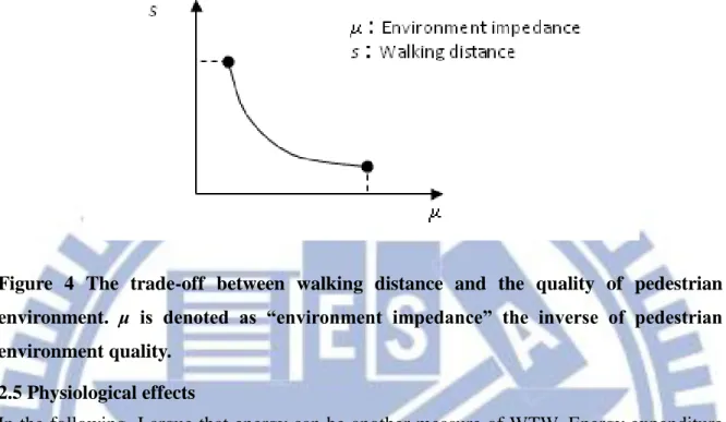
Environmental factors will affect the WTW. Weather is a critical factor (Pushkarev and Zupan, 1975; Zacharias, 2001), but so is the design of the pedestrian environment. In turn, a higher WTW can be considered as an effect of improved amenities from improvement projects. Studies have found that the average acceptable walking distance can be readily be extended by creating a pleasant environment in the urban space (Lövemark, 1972; Untermann, 1984), as shown in Figure 4. It should be noted however that the environmental effect has limits. The upward trend tends to peak at the greatest distance people are willing

(23)

12

to walk. In addition, the downward trend has a boundary as well, such as a bad street space where most pedestrians will not walk regardless of how short the distance is.

Figure 4 The trade-off between walking distance and the quality of pedestrian environment. μ is denoted as “environment impedance” the inverse of pedestrian environment quality.

2.5 Physiological effects

In the following, I argue that energy can be another measure of WTW. Energy expenditure is an important aspect of physiology. To measure WTW with energy, I must look toward the fields of exercise physiology and psychophysiology linking psychological perception and physiological response. The energy expenditure studies in exercise physiology have focused on specific groups (such as soldiers, people of a certain age group etc.), moving status (such as the walking speed), and the working environment (such as a moving platform to simulate ship motion) (Bastien et al., 2005; Demczuk, 1998; Heus et al., 1998; Rose et al., 1991). Methods to record EE often include the doubly labeled water technique, pedometers, oxygen consumption (VO₂), carbon production (VCO₂) and heart rate (HR). Among those, HR indicates the rate of oxygen consumption which relates linearly with HR (McArdle et al., 2007, pp. 206). It shows a close estimation and provides an affordable way to obtain reasonably accurate data in freely moving subjects (Spurr et al., 1988). Thus, this research uses HR to measure WEE.

Another question is how PEQ affects WEE through psychological perception. According to studies of psychophysiology, the effect from psychological perception can be observed by physiological measures, such as HR (Andreassi, 2007). HR indicates the arousal of the sympathetic nervous system (SNS). When a person walks on a street s/he perceives the PEQ,

(24)

13

and this perception produces a specific emotion. This emotion causes an arousal of the SNS. Psychophysiology studies found that a negative mood state (such as fear) significantly increases a person’s HR, thereby increasing energy expenditure at the same time. In contrast, a positive emotion, such as a pleasant feeling, will result in lowering the HR (Levenson et al., 1990). Since a good street environment results in pedestrians having a positive emotion, they spend less energy while walking.

2.6 Agent-based model in the dynamic pedestrian research

An ABM involves both the model and the simulator to observe the effect on the system of the interaction between agents as well as the interaction between agents and the environment (O’Sullivan and Haklay, 2000). The ABPM is one of the ABMs for pedestrians. Its strength lies in the use of fine-scale data and the “bottom-up” prediction (Bonabeau, 2002). Traditionally, the transportation models used the data scale to study pedestrians, but they focused more on O-D pair analysis and used a higher scale than the scale for walking (Batty, 2001). The traditional prediction models are aggregative and built with “top-down” thinking, while the emerging notion of prediction turns to the “bottom-up” thinking, where observed events are collected and to allow the development of superior systems. Thus, pedestrian movements can be simulated to predict a more global structure from the local action and reflect the actual characteristics of the local environment (Batty, 2005).

One issue when building an ABPM is how to choose a suitable scale for the spatial data. The types of spatial data in an ABPM can be categorized as discrete or continuous. Cellular automata (CA) is a widely-used discrete type ABPM and its successful application can be found in Batty (2005). Continuous spatial data can be found in studies using Cartesian coordinate system, like Helbing et al. (1995) or in flow analyses. The former marks space and location in a grid and may be too rough to observe any local congestions or the performance of the design. Therefore, continuous data is preferred in the present study. Agents, the environment and rules are the three components of the ABPM simulator (Epstein and Axtell, 1995). An agent of a pedestrian is coded by giving it human dimensions and behavioral characteristics, such as walking speed, body depth, shoulder width and personal space (Fruin, 1971). The range of these characteristics is large. Measures also vary across social factors and culture, and thus behavior characteristics should be surveyed to ensure they fit the local environment (Hall, 1966).

Environment in an ABPM refers to the artificial world for space and facilities. Recently, bottlenecks, room and channel have been simulated to observe the effects of geometrical

(25)

14

form (e.g., funnel), behavioral characteristics (e.g., visual perception) and collective behavior (e.g., lane formation) (Helbing et al., 2001; Turner and Penn, 2002; Isobe et al., 2004). It was found that the geometrical form of the design significantly affects a system’s performance. This finding indicates that congestion can be improved.

The behavior of agents is governed by a set of rules or a strategy. Maximizing utility and minimizing cost are often applied to analyze route choice (Antonini et al., 2006; Hoogendoorn and Bovy, 2005). Other objectives like minimum energy expenditure or keeping a desired speed, can be developed as strategies (Hsu and Tsai, 2010). Rules and strategies must be designed to fit the environment, because agents act for specific purposes. In this study, pedestrians pass each other in corridors by changing direction in order to bypass slow-walking pedestrians. This strategy can maximize spaciousness and it is discussed in the next section.

Applying an ABPM for a pedestrian corridor design is rarely found in the literature. The most relevant issue is the analysis by Helbing et al. (Helbing et al., 2005). They applied their “social force model” to the analysis of improving walkways, bottlenecks and intersections. They found that a series of columnar objects, e.g., a railing or a row of trees, in the middle of a road can stabilize a lane or a tunnel where impatient pedestrians try to overtake one another but are obstructed by the opposite stream. They also found that a funnel-shaped design can improve a pushy crowd. However, they did not offer any suggestions for dealing with the substantial difference in mobility, nor did they take the effect of reducing the effective width of the corridor into account.

2.7 Summary

In this chapter, I have reviewed the literature of WTW. This thesis integrated the statements from the published studies to make the rigorous definition to illustrate its relationship with street amenities. The previous studies mostly agree that better SA can enhance WTW within a range, but we need empirical evidences to conduct the following analyses. That is because only when the linearity between SA and WTW is ensured, the analyses and prediction can be conducted with Pandolf et al. and discrete choice models I used.

The characteristics of ABM are also reviewed to aid the following study. I first highlighted the advantage of ABM for the dynamic characteristics of pedestrians. The components of ABM generally include rule, scale and parameters. The third is important for the following ABM simulations, because the corridor is designed to reflect a population aging society. By these parameters, the following simulations can be conducted close to the real world. This

(26)

15

idea may not be new; in particular ABM recently receives much attention. However, its application for space design by comparing the mobility performances may be a new creation.

(27)

16

CHAPTER 3 ESTIMATING WALKING DISTANCE

To achieve the goals outlined in the previous sections, there are some methodologies designed in the following. The estimated walking distances are also shown to aid to practice.

3.1 Energy expenditure

Walking primarily costs the pedestrian time and physical effort (Pushkarev and Zupan, 1975), and a typical measurement of physical effort is energy expenditure (EE) (McArdle et al., 2007). Let’s introduce a “work” type equation, (1), to illustrate the process of EE:

   

t dt v

g m

e_w   



 r (1) where a pedestrian with a body weight m, walks with a speed function v

 

t on a sidewalk where the friction value at position

r

is 

 

r and g is the gravitational acceleration(9.8m/s2). If a pedestrian has been walking for a period of time t, the total amount of energy s/he consumed is about ew. If street environments can be categorized by

street types, then equation (1) can be rewritten as:



     P p p p w m g s e 1  (2)

where a route involves P types of streets, and sp is the walking distance of a pedestrian

walking at a constant velocity v for a period of time t on a type p street; and μp is the friction

on a type p street. If we sum the energy consumption for each type of street, then we get the total energy consumption ew. It is evident that there is a trade-off for the pedestrian between

s and μ under a given EE, as shown in Figure 3.

Pandolf et al. (1977) illustrated a WEE model from a physiological perspective:



/



( )(1.5 0.35 ) ) ( 2 5 . 1 m m l l m2 n m l v2 v G W         (3) where W is the metabolic rate or energy expenditure per second (J/s, watts) ; m is the body weight (kg); l is the load carried (kg); v is the velocity (m/s); G is the grade (%); and n is the terrain factor or friction. To determine the total amount of WEE, the metabolic rate needs to be multiplied by the walking time t:

t W

e_w   (4) where the unit of ew is in joule(J). Hall et al. (2004) compared the published energy

(28)

17

close to the actual value of the walking energy expenditure.

It is worthwhile to note that Pandolf et al. (1977) used two factors to reflect the environmental effects on WEE: terrain factor and grade. The terrain factor was originally defined as an additional WEE where pedestrians had to overcome the friction of the road surface, similar to friction μ in our equation (1). Several studies conducted experiments to establish a set of terrain factor values (n) based on the type of road surface, including blacktop (1), dirt road (1.1), light brush (1.2), heavy vegetation (1.5), swampy bog (1.8), loose sand (2.1) (Pandolf, et al., 1976; Soule and Goldman, 1972).

However, these values do not consider the effect of psychological perception, and the observed value (n~ ) measured from real streets may not be equal to the theoretical value that

were tested under controlled conditions (n~n). Thus, the terrain factor (nˆ ) needs to be

redefined and adjusted to reflect the actual characteristics of the real street space.

Thus, for the adjustment process we first take the terrain factor as an inverse function of equation (5):



W m l v G



f

n~ , , , , (5) A vector of variables x contributes to the variance of the terrain factor, except the variables in equation (5). These additional effects of the street’s amenities can be aggregated as parameter  for adjusting the theoretical value n to be the observed value(n~ n). The adjusting parameter can then be written as:







  x₁,x₂,...,x_M  (6) where 

 

x is a function consisting of a vector of street factors that significantly affect the WEE, M is the number of factors, and ε is the error term. In the walking spaces in urban areas, the road surface tends to be homogeneous, such as concrete, asphalt, brick etc. According to the previous definition, its theoretical value is similar to that of a treadmill or blacktop (n1). So the observed value can be shown as:

 



  

 1 x

~

n (7) The adjusted terrain factor can be estimated through 

 

x (nˆ

 

x ). Then equation (3) can be rewritten as:



/



 

( )(1.5 0.35 ) ) ( 2 5 . 1 m m l l m 2 m l v2 v G W    x     (8) and we can then use the modified model from Pandolf et al. (1977) to perform the following analyses.

In addition, this research introduces the “iso-energy curves” concept to enhance the WEE application. We have described a scenario where people are used to a certain amount of

(29)

18

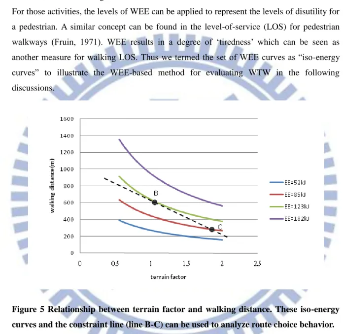
WEE. In reality, WEE varies greatly and depends on many factors, including trip purpose. A greater WEE, as shown in Figure 5 using Pandolf et al.’s (1977) model, implies that the pedestrians must expend more effort during walking. This may be unfavorable for some activities, like commuting.

For those activities, the levels of WEE can be applied to represent the levels of disutility for a pedestrian. A similar concept can be found in the level-of-service (LOS) for pedestrian walkways (Fruin, 1971). WEE results in a degree of ‘tiredness’ which can be seen as another measure for walking LOS. Thus we termed the set of WEE curves as “iso-energy curves” to illustrate the WEE-based method for evaluating WTW in the following discussions.

Figure 5 Relationship between terrain factor and walking distance. These iso-energy curves and the constraint line (line B-C) can be used to analyze route choice behavior. 3.2 Energy expenditure experiment

For the following energy expenditure analyses, the predictive function 

 

x needs to be established. Thus this research designed an experiment and would recruit 30 participants, 15 men and 15 women, to conduct experiments on seven distinct types of streets. In order to determine the effect of timing (day or evening) and to enlarge the sample size, the subjects would be asked to walk up and down each street, once during the daytime and once in the evening (after dark). Thus, a total of 840 samples would be collected to perform a regression analysis. It was a compromise necessitated by the limited budget.

(30)

19

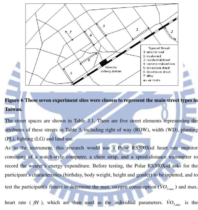
Streets of seven main types in Hsinchu City, Taiwan would be investigated in this experiment, including arterial roads, boulevards, residential streets, mixed-use streets, commercial parkways, downtown streets, and alleys (Marshall, 2005). The locations of those streets are shown in Figure 6.

Figure 6 These seven experiment sites were chosen to represent the main street types in Taiwan.

The street spaces are shown in Table 3.1. There are five street elements representing the attributes of these streets in Table 3, including right of way (ROW), width (WD), planting (PL), lighting (LG) and land use.

As to the instrument, this research would use a Polar RS300Xsd heart rate monitor consisting of a watch-style computer, a chest strap, and a speed-distance transmitter to record the wearer’s energy expenditure. Before testing, the Polar RS300Xsd asks for the participant’s characteristics (birthday, body weight, height and gender) to be inputted, and to test the participant’s fitness to determine the max. oxygen consumption (VO2_max) and max.

heart rate ( fH ), which are then used as the individual parameters. VO₂_max is the maximum capacity of the body to contain and utilize oxygen during incremental exercises. This capacity reflects the physical fitness of the individual and accounts for a significant portion of the variation in metabolic rate (Poehlman et al., 1990). The device also records the walking speed, walking time, and walking distance, all of which are required to analyze the terrain factor value through equation (8).

(31)

20

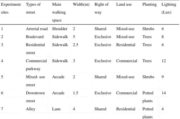
Table 2 Spatial characteristics of the experiment sites.

Experiment sites Types of street Main walking space Width(m) Right of way

Land use Planting Lighting (Lux)

1 Arterial road Shoulder 2 Shared Mixed-use Shrubs 6

2 Boulevard Sidewalk 5 Exclusive Mixed-use Trees 8

3 Residential

street

Sidewalk 2.5 Exclusive Residential Trees 6

4 Commercial

parkway

Sidewalk 3 Exclusive Commercial Trees 12

5 Mixed- use

street

Arcade 2 Shared Mixed-use Shrubs 9

6 Downtown

street

Arcade 1.5 Exclusive Commercial Potted

plants

14

7 Alley Lane 4 Shared Residential Potted

plants 4

Note: Width, right of way, land use, planting and lighting are independent variables of regression analysis. Their codes are shown in Table 5.

Prior to the tests, each participant would be informed as to the purpose of the experiment and received training in the operation of the Polar RS300Xsd. Then the subjects tested their personal VO₂_max value as the parameter for the device to compute the WEE while avoiding any distractions. Heavy physical exertion, smoking and consuming a large meal prior to the test are also avoided. The participants refrained from frequently visiting those streets prior to the test in order to avoid becoming too familiar with those sites, which could then result in a lower stimulus.

During walking, the participants would be asked to maintain as much possible a constant walking speed in order to reduce the inaccuracy resulting from using the mean walking speed as the input velocity v. In addition, the subjects would be asked to rest for ten minutes before their next test to avoid the effect of the previous walk influencing their metabolic rate in the next test. All experiments would be carried out in dry weather.

(32)

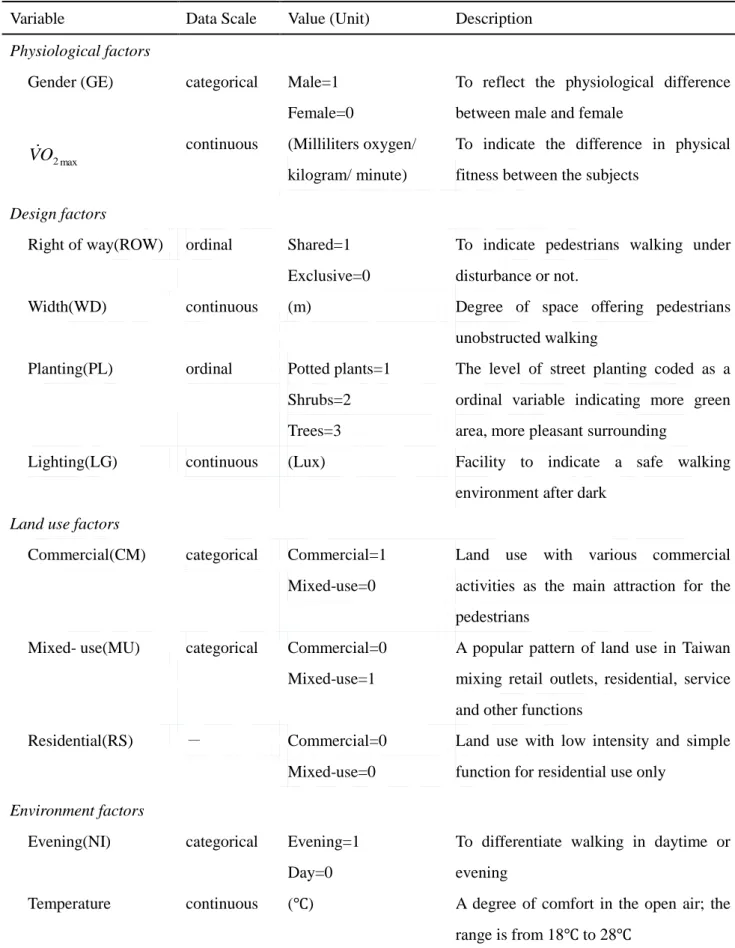
21 Table 3 Summary of independent variables.

Variable Data Scale Value (Unit) Description

Physiological factors

Gender (GE) categorical Male=1

Female=0

To reflect the physiological difference between male and female

max 2

O

V continuous (Milliliters oxygen/

kilogram/ minute)

To indicate the difference in physical fitness between the subjects

Design factors

Right of way(ROW) ordinal Shared=1

Exclusive=0

To indicate pedestrians walking under disturbance or not.

Width(WD) continuous (m) Degree of space offering pedestrians

unobstructed walking

Planting(PL) ordinal Potted plants=1

Shrubs=2 Trees=3

The level of street planting coded as a ordinal variable indicating more green area, more pleasant surrounding

Lighting(LG) continuous (Lux) Facility to indicate a safe walking

environment after dark

Land use factors

Commercial(CM) categorical Commercial=1 Mixed-use=0

Land use with various commercial activities as the main attraction for the pedestrians

Mixed- use(MU) categorical Commercial=0

Mixed-use=1

A popular pattern of land use in Taiwan mixing retail outlets, residential, service and other functions

Residential(RS) － Commercial=0

Mixed-use=0

Land use with low intensity and simple function for residential use only

Environment factors

Evening(NI) categorical Evening=1

Day=0

To differentiate walking in daytime or evening

Temperature continuous (℃) A degree of comfort in the open air; the

range is from 18℃ to 28℃

(33)

22

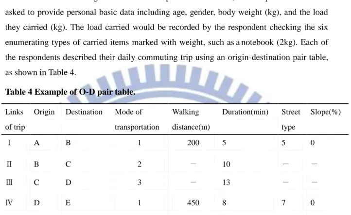
The questionnaire consists of basic personal data, origin-destination pair survey, and the street characteristics along the routes. For the personal basic data, each respondent would be asked to provide personal basic data including age, gender, body weight (kg), and the load they carried (kg). The load carried would be recorded by the respondent checking the six enumerating types of carried items marked with weight, such asanotebook (2kg). Each of the respondents described their daily commuting trip using an origin-destination pair table, as shown in Table 4.

Table 4 Example of O-D pair table.

Links of trip

Origin Destination Mode of transportation Walking distance(m) Duration(min) Street type Slope(%) Ⅰ A B 1 200 5 5 0 Ⅱ B C 2 － 10 －－ Ⅲ C D 3 － 13 －－ Ⅳ D E 1 450 8 7 0

Note: Mode of transportation, 1. walking, 2. bus, 3. rapid transit, 4. bicycle, 5. motorcycle.

Each respondent then identify all places they visited during their trip on a map (such as origin, transit stop, and destination) and then link them as a route. A commuting route might involve several links divided by mode of transport or street type, but the walking link is the only item of concern in this research. The participants would be asked to just write down the walking time for each link, and then I measure each walking distance. Walking velocity would be obtained by dividing each walking distance by the walking time. To compute the adjusted terrain factor value through equation (8), each respondent would mark down how they felt about the right of way, lighting, and planting (see Table 3) by check-marking the items which are shown complete with a sample photograph. For example, the respondents indicate the lighting level from a picture, and then the corresponding Lux number would be used as the input value.

It is unrealistic to assume that respondents can or will spend time on measuring VO₂_max

through a device during the interview. Fortunately, Shvartz and Reibold(1990) provides an age-based method to check the VO2_max value after the participant provides the information

(34)

23

This allows us to apply equation (8) to calculate the estimated metabolic rate and multiply it with the walking time in each street type. I then summed them using equation (4), and then estimate the walking energy expenditure for each commuting trip:



   K k k k w w t e 1 (9)

where K denotes the number of street types; w denotes the metabolic rate while walking _k

on a type k street, and t denotes the walking time on a type k street. _k

3.3 Results

Then a regression analysis was performed using SPSS 12.0 to establish the predictive model

 

x

 . The summary of the values for the observed terrain factors for the seven street sites are shown in Table 3.4. The regression analysis included two steps: the first step was to examine the statistical insignificance among the candidate variables. After deleting the insignificant variables, the second step in designing the predictive model was performed. As shown in Table 5, there is a difference in the ranking of the mean observed values between daytime and evening. In addition, each site shows substantial variation, implying that individual characteristics and timing may contribute at least in part to the effects. Thus, in addition to the five street factors, gender, VO₂_max, timing and temperature are also involved in step 1.

It must be noted that the coding method determined the final number of variables used in regression analysis. For example, we treated land use as a categorical (nominal) variable and coded it as a dummy variable, and it is therefore examined for two types of land use. Planting is assumed to be an ordinal variable because there is wide agreement that a greener area is more pleasing to pedestrians. A more detailed explanation of those variables is discussed in Table 6. A total of 10 candidate variables are used in the first step of the regression analysis.

Other coding methods such as effect coding are worth considering, but they must be designed to fit the surveyed pedestrian environment. For example, when using effect coding, the question is usually termed as “good, fair, poor”, and the codes may then be set as “+1, 0, -1”. However, this is more suitable for psychological measurement. Regarding planting (PL) in this research, green areas are available in most of our surveyed streets, so the question design actually focuses on how green the street is. Coding potted plant as -1 seems to be

(35)

24 unsuitable.

Table 6 shows that two personal physiological factors, gender (GE) and VO₂_max, are statistically significant. This suggests that the value of the terrain factor will significantly vary with gender and VO₂_max. A negative sign for the gender variable indicates that, when all other factors are equal, women expend more energy than men. It is probable that women generally have smaller muscle mass and produce less power, thus they put greater effort into the same movement. Kerr et al. (2001) found a similar phenomenon in stair-climbing: after placing motivating messages on the stair risers, men are significantly more willing to use stairs than women. Their finding confirms the effect of gender on WTW. VO2_max proves to

be strongly significant, suggesting that physical fitness is a determining factor for energy expenditure, and that VO₂_max reflects individual physical fitness rather than age.

Right of way (ROW) was found to be statistically significant, but the width of the walking space was not. These findings suggest that the range of walking space width (WD) from 1.5 to 5 m does not significantly affect the terrain factor. This is probably due to the fact that the testing range of the width of the walking spaces being tested was wide enough for most participants to walk unhindered. On the other hand, the disturbance from vehicles and incompatible activities significantly affected a pedestrian’s energy expenditure. Lighting (LG) had a negative sign and was significant, suggesting that good street lighting contributes greatly to the street amenity. It also suggested that heart rate increases significantly at night but declines when the lighting level is higher. Planting (PL) also shows a significant effect on WEE, confirming that the larger the green area, the higher the amenity of the street. Temperature is not statistically significant, possibly because the participants were used to the range of 18~28℃ weather and temperature did not significantly affect energy expenditure.

Walking in the evening (NI) causes a greater terrain factor value than during the daytime. It is possible that individuals must make more effort to understand the environment or are more concerned about personal safety when lighting levels are low. The greater effort results in a higher heart rate. Both land use factors (CM and MU) were not statistically significant, indicating that land use patterns did not lead to a significant difference in energy expenditure between the seven streets in our experiment.

(36)

25

At the second stage, we removed the insignificant variables and developed a terrain factor predictive function. This function was designed because some variables had independent effects while others reflected interactive effects. For example, lighting is used mainly after dark, and therefore the best calibrated predictive function of an adjusted terrain factor is shown as: 386 0 074 . 0 02 0 408 0 152 0 528 0 036 0 ˆ . VO₂_max . GE . ROW . NI . NI LG PL . n         (10)

where the fourth and fifth terms are designed for variables with interactive effects in which

NI is a dummy variable to reflect walking after dark (NI=1) or during daytime (NI=0). The

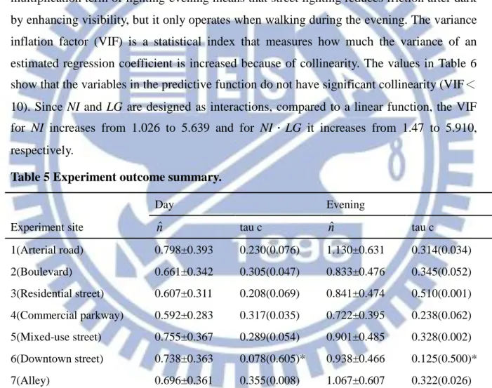
multiplication term of lighting-evening means that street lighting reduces friction after dark by enhancing visibility, but it only operates when walking during the evening. The variance inflation factor (VIF) is a statistical index that measures how much the variance of an estimated regression coefficient is increased because of collinearity. The values in Table 6 show that the variables in the predictive function do not have significant collinearity (VIF＜ 10). Since NI and LG are designed as interactions, compared to a linear function, the VIF for NI increases from 1.026 to 5.639 and for NI．LG it increases from 1.47 to 5.910, respectively.

Table 5 Experiment outcome summary.

Day Evening

Experiment site nˆ tau c nˆ tau c

1(Arterial road) 0.798±0.393 0.230(0.076) 1.130±0.631 0.314(0.034) 2(Boulevard) 0.661±0.342 0.305(0.047) 0.833±0.476 0.345(0.052) 3(Residential street) 0.607±0.311 0.208(0.069) 0.841±0.474 0.510(0.001) 4(Commercial parkway) 0.592±0.283 0.317(0.035) 0.722±0.395 0.238(0.062) 5(Mixed-use street) 0.755±0.367 0.289(0.054) 0.901±0.485 0.328(0.002) 6(Downtown street) 0.738±0.363 0.078(0.605)* 0.938±0.466 0.125(0.500)* 7(Alley) 0.696±0.361 0.355(0.008) 1.067±0.607 0.322(0.026)

Note: The adjusted terrain factor values (nˆ) are shown asmeanSD; tau c is shown as value (p-value) ; * not significant at the 10% level.

To determine the consistency between psychological perception and physiological response, the participants ranked all streets by preference (1~7). We then compared the data of the observed ranking of the terrain factor by means of Kendall's tau c test. As shown in Table 5,

考量街道寧適性下步行可及性與移動性之研究

國 立 交 通 大 學

運輸科技與管理學系

博 士 論 文

考量街道寧適性下步行可及性與移動性之研究

Walking Accessibility and Mobility with the Consideration of Street

Amenities

研 究 生：蔡耀慶

指導教授：許巧鶯 教授

考量街道寧適性下步行可及性與移動性之研究

Walking Accessibility and Mobility with the Consideration of Street

Amenities

研 究 生：蔡耀慶 Student：Yau-Ching Tsai

指導教授：許巧鶯 Advisor：Chaug-Ing Hsu

國 立 交 通 大 學

運 輸 科 技 與 管 理 學 系

博 士 論 文

誌 謝

感謝陪我走過這八年的許老師、我的家人、容瑛及研究室同仁（慧潔

學姐、剛伯學長、佳紋、憲梅、郁哲…），謝謝你們的包容與付出。感謝

指導過我的所有師長們：張新立院長、卓訓榮主任、吳水威老師、王晉元

老師、黃家耀老師…，提供行政協助的系辦助理們，以及在運輸年會一起

打拚過的學弟妺們。更要感謝四位口試委員：任維廉老師、林俊源老師、

林楨家老師以及金家禾老師，在口試時提供許多寶貴的建議。另外，我也

要謝謝交通處的所有同仁，跟你們共事是非常快樂的事。最後，感謝天主

～我終於畢業了！

TABLE OF CONTENTS

摘 要

ABSTRACT

LIST OF TABLES

LIST OF FIGURES

GLOSSARY OF SYMBOLS

 

r

 

 

CHAPTER 1 INTRODUCTION

CHAPTER 2 LITERATURE REVIEW

CHAPTER 3 ESTIMATING WALKING DISTANCE

   



 

r

 















 

 

 

 





 

 



 

國立交通大學

博士論文

研究生：蔡耀慶

指導教授：許巧鶯教授

研究生：蔡耀慶 Student：Yau-Ching Tsai

國立交通大學

運輸科技與管理學系

博士論文

誌謝

摘要