影響雙邊貿易因素之探討

全文

(1)國立高雄大學應用經濟學系碩士論文. 影響雙邊貿易因素之探討 On the Study of the Determination of Bilateral Trade Flows. 研究生：謝雅雯撰指導教授：鄭義暉博士. 中華民國九十八年七月.

(2) 誌謝詞轉眼間兩年的研究所生涯將告一段落，終於完成碩士學位的目標，這一路走來有苦、有樂，在論文完成的那一刻，真正感受到對自我的肯定與信心。在高雄大學應用經濟學系碩士班裡，感謝的人甚多，首先，承蒙恩師. 鄭義. 暉教授用心良苦的指導與照顧，總是不厭其煩地提供寶貴意見與建議，遇到問題的時候，老師總是細心地解說，直到我真正瞭解，讓我學習到面對問題的處理方式，受用無窮，在此由衰地感謝老師。論文審查期間，感謝山大學政治經濟學系. 蔡穎義教授以及中. 吳世傑教授百忙中抽空審查並細心斧正，使論文更加完. 整，在此亦表達最誠摯的謝意。另外感謝. 許聖章老師指導計量方法之處理概念。. 論文撰寫過程中特別感謝陪我度過艱苦時光的同學：顯捷、裕傑、瑞樺、本謙、岱吟、偲驊、姎凌，及系上人員：姿宇姐、珮瑜姐，回憶起這段互相砥礪課業的時光，讓我在學業上才能順利過關。另外，擔任一年的會計學助教，實在是個難得的寶貴經驗，建立更多上台的膽量與台風。最後，由衰地感謝我的父母一路的栽培，不僅是生活上的支持，還有精神上的鼓勵，讓我無後顧之憂專心求學，也非常感謝老哥總是默默的支持與關心。由於大家的協助，才能順利完成碩士學位，總之謝謝大家，希望未來能有再聚首的一天。. 謝雅雯. 謹誌. 2009 年盛夏于高雄.

(3) 影響雙邊貿易因素之探討指導教授：鄭義暉博士國立高雄大學應用經濟學系學生：謝雅雯國立高雄大學應用經濟學系碩士班. 摘要現今透過國際間簽訂貿易協定以達成區域內消除大部分貿易障礙及非貿易障礙，進而增進會員國間之貿易量。本研究主要利用引力模型分析雙邊貿易流量之決定因素，當今主要貿易聯盟，包括北美自由貿易區、歐盟、歐元區、東協自由貿易區及南方共同市場，以採用虛擬變數之方式，針對 1986 年至 2006 年間各區域經濟整合體會員國及非會員國出口貿易流量進行實證分析，並利用經濟發展程度及產業內貿易指數將國家區分為不同群組，以探討雙邊貿易流量是否會因不同之經濟發展程度及產業內貿易指數水準而有明顯差異？實證結果顯示，在貿易國雙方皆為開發中國家，GDP 對雙方出口量所帶來的影響，相較之下，其影響高於貿易國雙方皆為已開發國家。在產業內貿易指數較高的貿易下，若貿易國雙方皆同屬北美自由貿易區、東協自由貿易區或南方共同市場時，對出口量有顯著正向關係。然而，貿易國雙方同屬 EU 或 EURO 成員國時，在不同的模型下，其所估計的結果卻不一致。. 關鍵字：雙邊貿易、引力模型、區域經濟整合、產業內貿易.

(4) On the Study of the Determination of Bilateral Trade Flows Advisor：Dr. I-Hui Cheng. Department of Applied Economics National University of Kaohsiung MA Student：Ya-Wen Hsieh. Department of Applied Economics National University of Kaohsiung. Abstract This dissertation uses various specifications of the gravity model of trade, and compares the results. In this study, each specification of estimation includes five trade bloc dummies to investigate the effects of bilateral trade with different levels of economic development and intra-industry index. The estimation results indicate that the coefficients of exporter’s and importer’s GDPs are higher for the case where both exporting country and importing country are developing countries, compared to the case where both exporting country and importing country are developed countries. From the results for the higher IIT trade flows, the within-bloc effect of NAFTA, AFTA and MERCOSUR is strictly positive and statistically significant. However, the intra-bloc effect of EU or EURO is ambiguous under different specifications.. Keywords: Bilateral trade, Gravity model, Regional economic integration, Intra-industry index, IIT.

(5) Contents. List Contents. i. List of Tables. ii. I.. Introduction. 1. 1. Motivation. 1. 2. Primary objective. 3. II.. The literature. 5. III.. Contemporary world trade. 11. IV.. Data and estimation models. 16. 1. The data. 16. 2. The models. 19. Estimation results. 24. V.. 1. The results for the PCS, Three-way FE and Two-way FE 25. gravity models 2. Estimation results – Using disaggregate data with different 28. levels of economic development 3. Estimation results – Using disaggregate data with different 33. IIT levels VI.. Conclusions. 36. Data Appendix. 40. References. 41. i.

(6) List of Tables Table 1. The total value of exports in different geographical regions. 45. Table 2. The total value of imports in different geographical regions. 46. Table 3. Exports of trade groups. 47. Table 4. Imports of trade groups. 48. Table 5. Intra-trade of trade groups. 49. Table 6. Export structure by partner: By main region of destination. 50. Table 7. Import structure by partner: By main region of destination. 51. Table 8. Variables and data sources. 52. Table 9. List of 41 exporting and 57 importing countries. 53. Table 10. Trade blocs and selected member countries. 54. Table 11. List of developed and developing countries and country dummies used in the estimation. 55. Table 12. Regression results for various models. 57. Table 13. Results from the gravity estimation – Both exporting and importing countries are developed countries. 58. Table 14. Results from the gravity estimation – Both exporting and importing countries are developing countries. 59. Table 15. Results from the gravity estimation – Exporting and importing countries are developed countries and developing countries respectively. 60. Table 16. Results from the gravity estimation – Exporting and importing countries are developing countries and developed countries respectively. 61. Table 17. The estimation results with IIT between 0.75 and 1. 62. Table 18. The estimation results with IIT between 0 and 0.25. 63. Table 19. The estimation results with IIT between 0. 5 and 0.75. 64. Table 20. The estimation results with IIT between 0. 25 and 0.5. 65. ii.

(7) I.. Introduction. 1. Motivation During the last twenty years, the development of the growing preferential trading agreements (PTA) has attracted great attention. By forming PTAs, many countries eliminate tariff, or lower trade barriers against their trading partners. There are various forms of PTA, e.g. free trade area (FTA), customs union (CU), common market and monetary union, which are classified according to the degree of economic integration among members. For example, in Africa, the most acting PTA is the Common Market of Eastern and Southern Africa (COMESA). In America, there are the Common Markets of the South (MERCOSUR), the North American Free Trade Agreement (NAFTA), the Central American Common Market (CACM), and Latin America Free Trade Association (LAFTA). In Asia, the Association of Southeast Nations (ASEAN) and then the ASEAN Free Trade Area (AFTA) has been working. In Europe, there are the Europe Union (EU), EURO area and the European Free Trade Association (EFTA). Since its accession to the General Agreement on Tariffs and Trade (GATT) in 1967, the World Trade Organization (WTO) was concluded in 1994 and entered into force on 1 January 1995. The WTO deals with the rules of fair trade between regions or countries, including agriculture, textiles and clothing, telecommunications,. 1.

(8) government purchases, industrial standards and product safety, food sanitation regulations, intellectual property, etc. By following the most-favored nation (MFN) principle, i.e. a country imposes a lower customs duty rate for any country and should treat the other trading partners equally, countries cannot discriminate between their trading partners. Thus, many countries have intention to integrate their markets. Regional trading agreements (RTAs) have become a very prominent feature of the multilateral trading system (MTS) in recent years. Based on the WTO statistics, there are more than 421 RTAs being notified to the GATT/WTO during 1990-2008, in which 324 RTAs are notified under Article XXIV of the GATT 1947, and 230 agreements are in force during the same period. Also, there are about 400 RTAs which continue and are scheduled to be implemented by 2010. Of these RTAs, FTAs account for over 90%, while CUs account for less than 10%. The latest formed RTA is Australia-Chile FTA & Economic Integration Agreement (EIA) which goes into effect on March 2009. Economists have been interested in estimating the impact of regional economic integration on trade flows, because volume of trade plays an important role in determining the aggregate welfare, which is counted by the summation of total consumption, investment, government expenditure and net foreign trade. Wonnacott and Lutz (1987), Krugman (1991), and Summers (1991) propose geographical. 2.

(9) proximity as a key predictor of trade creation and welfare improvement in PTAs. Krishna (2005) discusses the design of welfare-improving PTAs that ensure gains for member countries without negative impacting the outside countries. Krishna (2005) finds that there exists a significant effect of trade creation and trade diversion associated with preferential tariff liberalization against partner countries. In addition, the correlation between the welfare change from preferential tariff reduction and distance is statistically insignificant, and unable to reject the null that distance does not matter. To outline the effects of RTAs on trade, this study reviews the world trade trend after year 1980 and considers whether the bilateral trade flows are affected by RTAs. This study intends to discuss the trend of the effects of regional blocs, particularly taking account of different levels of economic development and intra-industry trade to investigate the effects of regional economic agreements on trade volumes.. 2. Primary objective This dissertation focuses on the following issues. First, it attempts to study the determinations of trade flows using traditional and modified models of gravity type. Second, it considers whether the bilateral trade flows are affected by trading agreements. Third, the study further distinguishes how different levels of economic. 3.

(10) development affects bilateral trade flows. Fourth, this study measures how different level of intra-industry trade (IIT) has impact on bilateral trade.1 This dissertation is organized as follows. Chapter II presents the literature reviews. In Chapter III, the study mainly demonstrates the current world trade. In Chapter IV, the study discusses the estimation data and models, and Chapter V provides the empirical analysis. Concluding remarks are provided in Chapter VI.. 1 A standard measure of intra-industry trade is the Grubel-Lloyd (1975) index. A higher IIT indicates more intra-industry trade between two countries, and otherwise more inter-industry trade.. 4.

(11) II.. The Literature. The economic model of gravity type has been widely used for the study of bilateral trade flows, since it was introduced by Tinbergen (1962) and Pöyhönen (1963). The gravity model of the simplest type explains that trade flows between countries are determined by their sizes (as measured by its national incomes), and the cost of transportation between them (as measured by the distance between their economic centers). The modified version of Linnemann (1966) indicates population as an additional measure of country size, and predicts that the size of population has a significant and negative impact on trade flows. 2 It is also common to specify a gravity model including per capita income, which captures the similar effect of purchasing power on trade flows. By adopting the specification of the gravity model in which includes either population or per capita income, the purpose is to allow for non-homothetic preferences in the importing country, and to proxy for the capital/labour ratio in the exporting country (see Bergstrand, 1989). As shown in Brada and Mendez (1983), per capita national incomes have positive effects on trade flows. Normally, models of the gravity type consist of other explanatory variables to capture the effects of regional trading groups, political blocs, and various trade. 2. For recent uses of the gravity model with population, see Oguledo and MacPhee (1994), Boisso and Ferrantino (1997), and Bayoumi and Eichengreen (1997). 5.

(12) distortions. 3 The events and policies modeled as deviations from the value of trade predicted by the baseline gravity model are captured by dummy variables. As noted in Eichengreen and Irwin (1998), the gravity model is acting as “workhorse of empirical studies (of regional integration) to the virtual exclusion of other approaches.” Anderson (1979) considers the properties of the expenditure system to analyze the gravity model. Two cases of product differentiation are discussed in his study: the Cobb-Douglas (C-D) and constant-elasticity-of-substitution (CES) preferences. Bergstrand (1985) firstly includes the variables of prices, and adopts CES preferences to derive the gravity equation. Further, Bergstrand (1989) uses Dixit-Stiglitz preferences, i.e. products are differentiated among firms rather than countries, to consider the role of monopolistic competition in international trade. Baier and Bergstrand (2001), Eaton and Kortum (2002), and Anderson and van Wincoop (2003) consider that prices always adjust to equate supply and demand. The results in their studies show that price variables are powerful in explaining trade flows between countries. Deardoff (1988) derives bilateral trade relationship with the Heckscher-Ohlin and considering two cases, the frictionless trade and the impeded trade cases. He shows that in the presence of transportation costs and tariffs, trade flows on a C.I.F.. 3. See Bergstrand (1985, 1998) for imperfect competition. 6.

(13) basis will be the same form with the frictionless trade case. With C-D preferences, trade flows on an F.O.B. basis of the gravity equation are represented, weighed with the iceberg-form transportation costs. 4 With CES preference the measurement of the value of trade flows on an F.O.B. basis is more complicated. Trade flows are derived as function of the incomes of importing and exporting countries, exporter’s share of world income, the relative and average distances from suppliers. Under the assumptions of the identical and homothetic preferences without transportation costs and tariffs, both Anderson (1979) and Deardoff (1998) show that the gravity model is the product of the two countries’ incomes divided by the sum of world income. Bergstrand (1985) further imposes an additional assumption of perfect substitutability of goods internationally in production and consumption, and shows the value of a trade flow is simple one half of the square root of the product of the two countries’ incomes. Estimating the impact of regional economic integration on trade flows is that trade flow effects play an important part in determining the aggregate welfare change for members of a regional integration agreement. Viner (1950) introduces the concepts of trade creation and trade diversion effects to identify situations under. 4. Transportation costs for iceberg type between two regions are a proportion of goods shipped arrive in the importing country. 7.

(14) which a customs union (CU) is welfare-increasing or welfare-reducing. 5 Viner considers the case that the tariff is removed or eliminated between members as part of a free trade agreement while tariffs are maintaining against other countries. The issue of testing the effects of regional integration agreement on trade is of great concern due to the increasing tendency of countries to form preferential trading agreements in recent decades. The commonly used method in recent empirical literature is to estimate trade flows by the use of a dummy variable to identify regional integration agreement partners with simple gravity models, which can be used to address the effect of a regional trade agreement on the direction of trade. A regional integration agreement dummy variable takes the value of one if both trading partners interact in the same trading bloc and zero otherwise. 6 Aitken (1973) initially includes one dummy variable to the gravity model to evaluate the intra-bloc effect of a PTA, arguing that the European Community (EC) has statistically significant impact on trade flow between members. 7 Bayoumi and Eichengreen (1997) and Frankel (1997) propose two dummy variables for each PTA to evaluate the effects on intra-bloc and extra-bloc trade. One of the two dummy variables is set to be one if the two countries. 5. For a country, trade creation means that joining a customs union would have advantages if joining results in the replacement of high-cost domestic production by imports from a lower-cost country within the union. By contrast, trade diversion means that joining leads to a shift in domestic consumption from a low-cost country outside the customs union to a higher-cost country inside the union, the home country may suffer. 6 See Aitken (1973), Winters (1992), Bayoumi and Eichengreen (1997) and Sapir (1997) for the analysis of integration schemes in Western Europe. 7 Also see Abrams (1980) and Brada and Mendez (1985). 8.

(15) join the same trade blocs. Another dummy variable is set to be one if either country in the blocs. Then, the coefficients can be used to evaluate the trade creation and trade diversion. Soloaga and Winters (2001) includes three dummy variables for each trade bloc. To extend the basic gravity model by defining three sets of dummy variables for each trade bloc: one captures intra-bloc trade, a second captures imports by members from all countries (include members and non-members), and a third captures exports by bloc members to all countries (see Cheng and Tsai, 2008). Brada and Mendez (1983) uses a gravity model to examine the PTA effect, and note that economic integration tends to increase trade between member countries, and trade increases with their per capita incomes and decreases with the distance between them. Frankel (1995) includes additional dummy variables for country pair which shares a common land border and common language, and trade bloc dummy variables which evaluate the effect of free trade agreements. Frankel (1997) finds the MERCOSUR to have a significant and positive effect, and the EC to have a significant and negative effect between members in certain years (including four years, 1970, 1980, 1990 and 1992). A gravity model has where been used to examine Japanese trade by Eaton and Tamura (1994), who look at differences between Japanese and the United Sates trade and direct foreign investment patterns. Sawyer and Sprinkle (1997) survey the empirical literature of international economics. 9.

(16) regarding to Japanese trade. Baier and Bergstrand (2007) estimate the effects of FTAs on bilateral trade flows using a panel of cross section and time series data from year 1960 to year 2000, and find that the effect of an FTA approximately doubles the bilateral trade flows between two members after ten years.. 10.

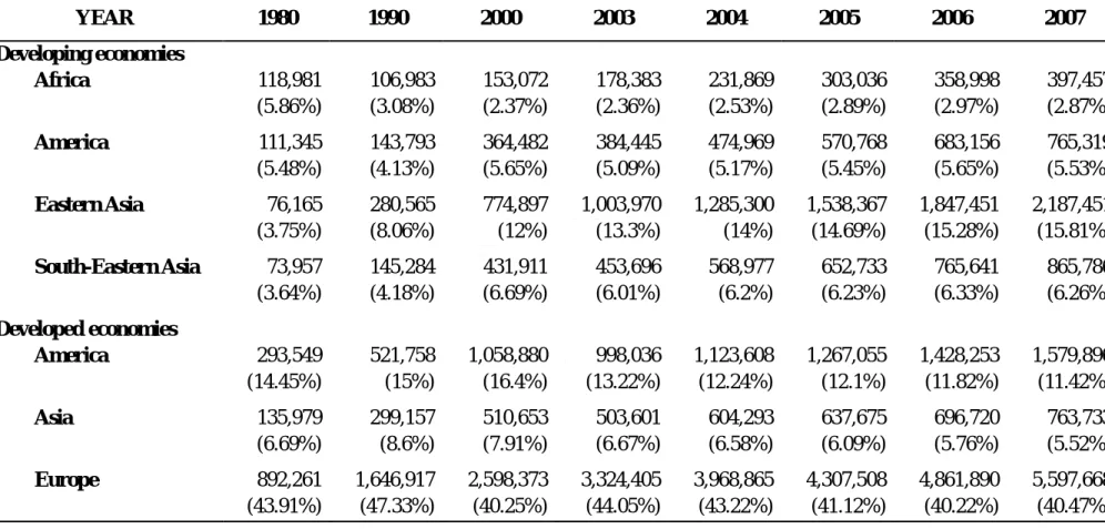
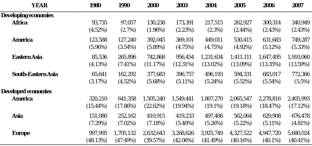
(17) III.. Contemporary World Trade. All the values of exports and imports in different geographical regions during year 1980 to year 2007 have grown significantly (see Tables 1 and 2). Since year 1980, the shares of exports and imports of developed Europe relative to world trade are consistently stable, being the highest during this period. As shown in Table 1, the share of the developed Europe’s exports relative to world trade is nearly 40.5 per cent in year 2007. It ranks the first in the world trade but is 3 per cent lower than that in year 1980. During the same period, in contrast, the export share of developing Eastern Asia has risen approximately five times, from 3.75 per cent in year 1980 to 15.8 per cent in year 2007, increasing fast up to 2,198,451 millions of dollars from 76,165 millions of dollars during year 1980 to year 2007. It is also shown that the value of exports in developing South-Eastern Asian and developed American countries have increased during this period. Note that the shares of exports of developing South-Eastern Asia is consistently increasing, contrasting that of developing America tends to be decreasing. As illustrated in Table 2, since year 1980 the shares of imports in different geographical regions also have shown similar trend as exports except America. The share of the developed America’s imports relative to world trade has risen during year 1980 to year 2007, but that of the developing America has declined. The share of the. 11.

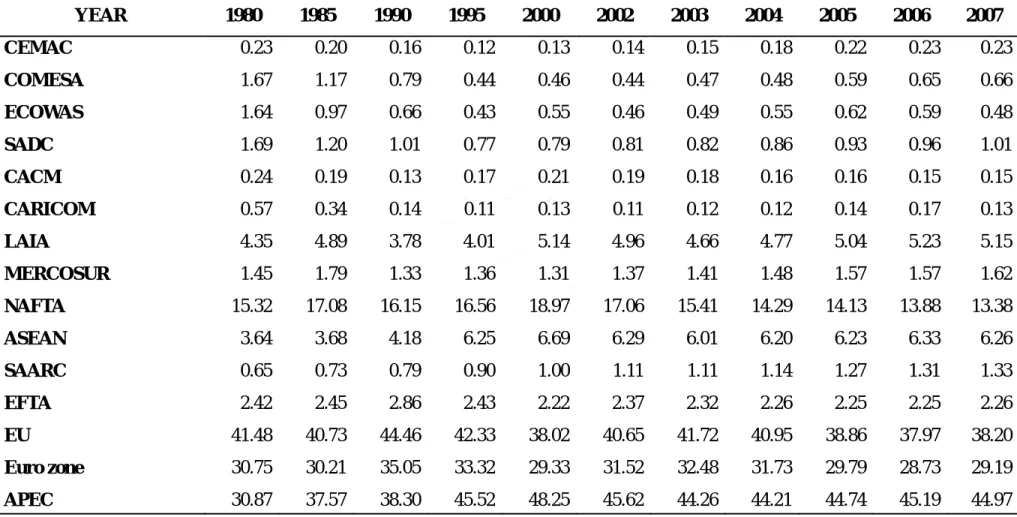
(18) developed Europe’s imports relative to world trade is nearly 40.5 per cent in year 2007. It still ranks the first in the world trade but is 8 per cent lower than that in year 1980, increasing to 5,680,024 millions of dollars from 997,995 millions of dollars during the same period. Similarly, the import share of developing Eastern Asia has risen almost four times, from 4.13 per cent in year 1980 to 13.59 per cent in year 2007, increasing to 1,910,060 millions of dollars from 85,536 millions of dollars. Also in Table 2, the share of developing South-Eastern Asian imports has increased, while the share of the developed Asia has declined. The shares of exports and imports relative to the world trade have increased in some trade groups between year 1980 and year 2007. In Tables 3 and 4, the shares of the European Union (EU) exports and imports are significantly higher than the other trade groups. As shown in Table 3, exports of the North American Free Trade Agreement (NAFTA) and Euro zone contribute to a large share of world exports, peaking to the highest in year 2000. During year 1980 to year 2007, the export share of the South Asia Association for Regional Cooperation (SAARC) has risen approximately two times, from 0.65 per cent in year 1980 to 1.33 per cent in year 2007. The shares of exports in the Association of South East Asian Nations (ASEAN) and Asian Pacific Economic Cooperation (APEC) have also increased during the same period. In contrast, the export share of the Caribbean Community and Common. 12.

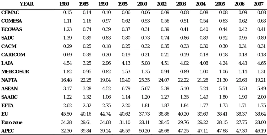
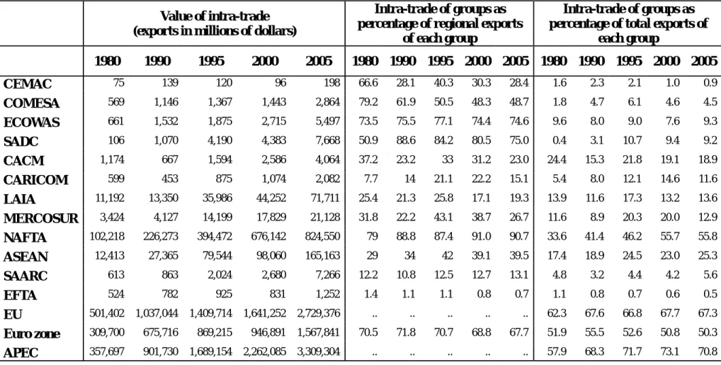
(19) Market (CARICOM) tends to be decreasing during the same period. With the exception of the Central American Common Market (CACM), CARICOM, NAFTA, APEC, the shares of imports in other trade groups in year 2007 are less than the shares of exports in the same year (see Tables 3 and 4). Table 5 shows the intra-trade in different trade groups between year 1980 and year 2005. As shown, the EU is the trade group which had relatively intense intra-trade during year 1980 and year 1990, and its share of intra-trade exports relative to trade with the rest of world is more than 62 per cent. During year 1995 and year 2005, APEC countries have more intense intra-trade than the other trade groups, and their intra-trade export is more than 70 per cent of total trade. Countries in these groups tend to trade more with members than with non-members. This seems particularly the case with trade blocs in the Euro zone, NAFTA, SADC and ECOWAS. The intra-trade of groups as percentage of regional exports in these groups are nearly 70 per cent to 90 per cent during this period. The share of intra-trade of groups as a percentage of regional exports in the NAFTA always ranks the first in the world, increasing up to 90.7 per cent in year 2005 from 79 per cent in year 1980. The intra-bloc trade of the CARICOM as percentage of regional exports has grown fast up to 15.1 per cent in year 2005 from 7.7 per cent in year 1980. Tables 6 and 7 show that the export and import structures of ASEAN countries,. 13.

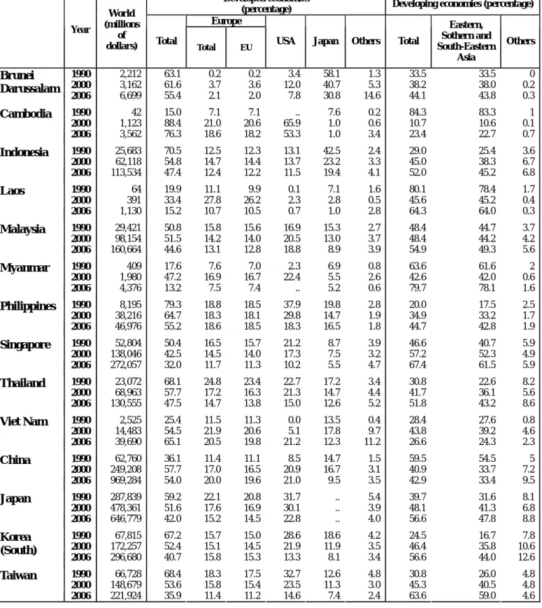
(20) China, Japan, and South Korea (ASEAN +3) with main region trade partners during year 1990 and year 2006. Note that the developed economies in these blocs include the Europe, USA, and Japan, and developing economies include the Eastern, Southern and South-Eastern Asian countries. Since year 1990, Japan’s exports to and imports from the rest of the world are the highest among ASEAN +3 countries. However, the values of China’s exports and imports rank the first in the ASEAN +3 in year 2006 (see the third columns of total Tables 6 and 7). As seen in Table 6, the Viet Nam’s and China’s exports to the rest of the world have risen approximately 16 times during year 1990 and year 2006. The export of Viet Nam has increased to 39,690 millions of dollars in year 2006 from 2,525 millions of dollars in year 1990. The export of China has increased to 969,284 millions of dollars in year 2006 from 62,760 millions of dollars in year 1990. The export share of Cambodia to the developing economies relative to the world trade is 84 per cent in year 1990, and to the developed economies are 88 per cent in year 2000 and 76 per cent in year 2006. As shown, the export shares of the ASEAN +3 countries have relatively intense trade with Eastern, Southern and South-Eastern Asia than other regions. It is also shown that most of these countries trend to increase the export to developing economies and decrease the export to developed economies. The export destinations of the Philippines and Indonesia have most changed during year 1990 and. 14.

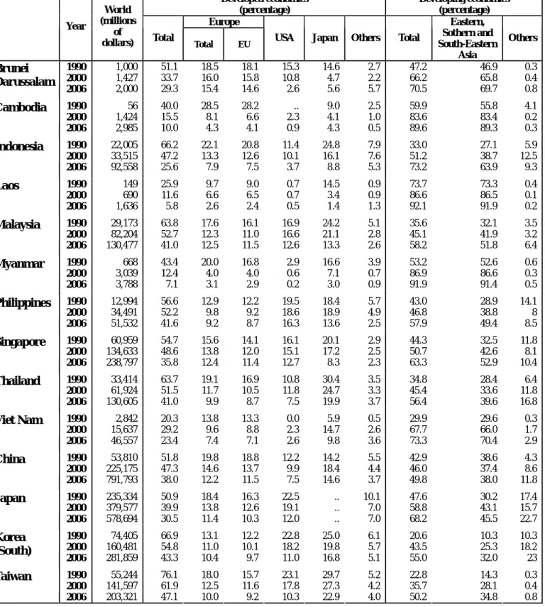
(21) year 2006. The Philippines’s export ratio of developed to developing economics is 79 to 20 in year 1990, and the ratio is 55.2 to 44.7 in year 2006. The Indonesia’s export shares of developed and developing economies are 70.5 per cent and 29 per cent in year 1990, and the shares of developed and developing economies are 47.4 per cent and 52 per cent in year 2006. In Table 7, the import shares of Laos and Myanmar relative to the Eastern, Southern and South-Eastern Asia are almost to 92 per cent in year 2006. In Singapore, there exists 54.7 per cent of its imports in year 1990 from developed countries, dropping to 35.8 per cent in year 2006. The import shares of China are consistently stable between 42.9 per cent and 49.8 per cent during year 1990 to year 2006. Surprisingly, the imports of Cambodia have risen almost 53 times, from 56 millions of dollars in year 1990 to 2,985 millions of dollars in year 2006.. 15.

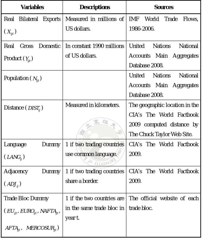
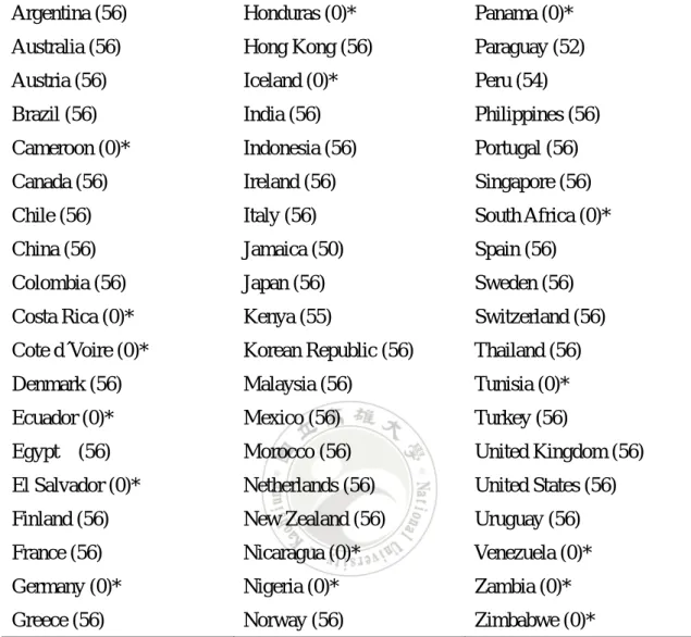
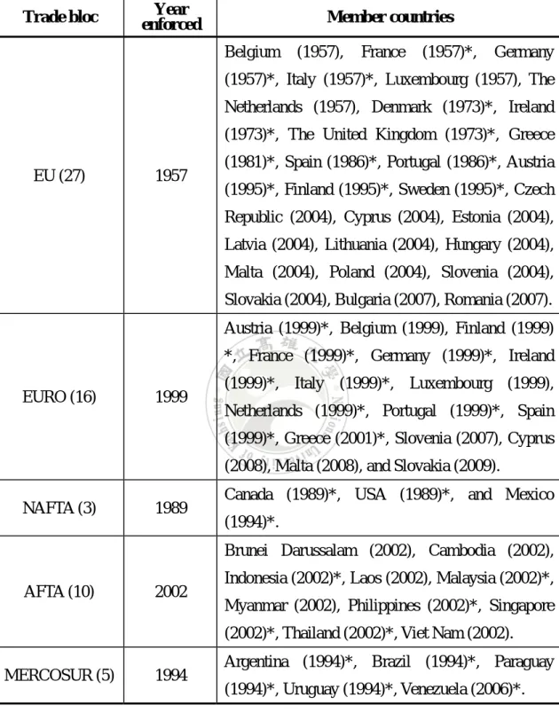
(22) IV.. The Data and Empirical Models. 1. The data Following most of the literature, this study uses the F.O.B. values of bilateral exports as the dependent variable. The independent variables include real GDP, population, the distance between geographical centers of two trading countries, and the dummy variables to indicate if two countries’ official languages are the same, two countries share a common border, and join the same trading bloc. Short descriptions of these variables and the sources are provided in Table 8. The data set used in this study is a balanced panel with 47,922 observations, which widely covers countries at different level of economic development and performance during the period 1986-2006. In each year, there are 2282 country trading pairs of 41 exporting and 57 importing countries. Table 9 demonstrates the list of the exporting and importing countries included in the study. To focus the effect of regional blocs, this study employs five regional bloc dummy variables, namely the European Union (EU), Euro area (EURO), North American Free Trade Agreement (NAFTA), ASEAN Free Trade Area (AFTA), and the South American Common Market (MERCOSUR). Descriptions of the each regional bloc’s year entered in force and its members are noted in Table 10. In this study, I assign a trading bloc dummy equal to one if two countries are acting in a same trade bloc in a given year. Since 1950, the European Coal and Steel. 16.

(23) Community (ECSC) were formed to unite economic power among member countries. European Economic Community (EEC) came into effect in 1957. The six founders are Belgium, France, Germany, Italy, Luxembourg and the Netherlands. Denmark, Ireland and the United Kingdom joined the EEC in 1973, Greece in 1981, and Spain and Portugal in 1986. In 1995, Austria, Finland and Sweden joined the EU in which member countries already enhanced their cooperative agreement after year 1992. In 2004, eight countries of central and eastern European countries join the EU, including Czech Republic, Estonia, Latvia, Lithuania, Hungary, Poland, Slovenia and Slovakia. Bulgaria and Romania joined the EU in 2007. In this study, the EU dummy is set to be one when two countries are acting in the EU in year t. The Euro area is a currency union that people use the Euro instead of their earlier official currencies. After EURO goes into effect in 1999, there are 16 EU countries joining the economic and monetary union during 1999-2009. a In 1999, Austria, Belgium, Finland, France, Germany, Ireland, Italy, Luxembourg, the Netherlands, Portugal and Spain have adopted the euro as their sole legal tender. Greece became one of EURO member countries in 2001. Slovenia adopted the euro as the official currency in 2007, Cyprus and Malta in 2008, and Slovakia was admitted in 2009. To consider the monetary effect of the EU on trade flows, this study uses a dummy to indicate if two countries are using the Euro, i.e. the EURO dummy is set to be one. 17.

(24) when two countries are commonly using Euro as their official currency. The Canada–US Free Trade Agreement (CUFTA) was formed in 1989. Then, the agreement was extended to include Mexico after the North American Free Trade Agreement entered into effect in 1994. To estimate this effect, in this study the NAFTA dummy takes the value of one for bilateral trade between the United States and Canada in 1989-1993, and the trade between Mexico, the United States and Canada during 1994-2006. The Association of Southeast Asian Nations (ASEAN) was established in 1967 by the five original member countries, including Indonesia, Malaysia, the Philippines, Singapore, and Thailand. Brunei Darussalam became the sixth member of the ASEAN in 1984, and Vietnam in 1995, Laos and Myanmar in 1997, and Cambodia joined the ASEAN in 1999. The ASEAN Free Trade Area (AFTA) was formed to liberalize trade among the ASEAN countries went into force in 2002. In this study, the AFTA dummy takes the value of one for bilateral trade between the ten members during 2002-2006. The MERCOSUR was created by four South American countries (Argentina, Brazil, Paraguay and Uruguay) in 1994, and Venezuela joined it in 2006. To estimate the effect, I use the MERCOSUR dummy by setting the value of one between Argentina, Brazil, Paraguay and Uruguay for 1994-2006, and between Argentina, Brazil, Paraguay, Uruguay and Venezuela for 2006.. 18.

(25) To control for different levels of economic performance, this study uses dummies to indicate if a country is developed or developing country in a given year. According to the CIA’s The World Factbook 2008, a country is defined as a developed country (a high-income economy) if its gross national income (GNI) in year 2005 was higher than and equal to $10,726, otherwise denoted as a developing country. Table 11 shows the developed and developing countries used in the estimation. The 24 developed countries are Australia, Austria, Canada, Denmark, Finland, France, Germany, Greece, Hong Kong, Iceland, Ireland, Italy, Japan, Korea, the Netherlands, New Zealand, Norway, Portugal, Singapore, Spain, Sweden, Switzerland, the United Kingdom, and the United States. Note that all of the developed economies listed in Table 11 have 2-way bilateral trade, but Germany’s and Iceland’s data are trade destination only.. 2. The models This study uses the various forms of the gravity model to analyze the determination of bilateral trade flows. The gravity model of international trade assumes that the value of bilateral trade flows can be estimated as an increasing function of the sizes of trading economies, a decreasing function of the geographic distance between them, and as a function of other economic and non-economic factors, which may enhance or deter bilateral trade. The gravity equation commonly used to international trade flows. 19.

(26) takes the following form: 8 ln X ijt = α 0 + β1 ln Yit + β 2 ln Y jt + β3 ln DISTij + β 4 LANGij + β5 ADJ ij + β 6 FTAijt + ε ijt ,. (CS). where X ijt is the value of exports from country i to country j in year t, Yit and Y jt are country i ’s and j ’s gross domestic products (GDP) respectively, DISTij is. the distance between the economic centers of country i and country j , LANGij is a dummy variable assuming the value of 1 if two countries use a common official language and 0 otherwise, ADJ ij is a dummy variable assuming the value of 1 if two countries share a common land border and 0 otherwise, and FTAijt is a dummy variable assuming the value of 1 if the two countries join a trade bloc in year t and 0 otherwise. ε ijt is the residual term of estimation equation. The CS model is normally estimated by the ordinary least squares (OLS) method. This study makes comparison between the estimation results of various forms of gravity models. A pooled cross-section model is used to serve as the benchmark. Then, a three-way fixed effects model suggested by Mátyás (1998) with time-invariant variables is estimated for comparison. Finally, another specification of two-way fixed effects model suggested by Cheng and Wall (2005) is also estimated, and to be compared to the model of Mátyás type without time-invariant variables.. 8. The standard gravity equation may include exporter’s and importer’s populations, or their per capita GDPs. 20.

(27) (1) The conventional gravity model Undoubtedly, pooling cross-section and time-series data increases the number of data point for estimation. The pooled cross-section model (PCS) deals with the problem of additional degrees of freedom without greatly increasing the number of variables, allowing for the intercepts to differ over time. To estimate the effects of trade blocs on bilateral trading pattern, the gravity model can be specified as: ln X ijt = α t + β1 ln Yit + β 2 ln Y jt + β 3 ln N it + β 4 ln N jt + β5 ln DISTij + β 6 LANGij + β 7 ADJ ij. (PCS). + β8 EU ijt + β9 EUROijt + β10 NAFTAijt + β11 AFTAijt + β12 MERCOSURijt + ε ijt ,. where α t is the year-specific effect common to all trading pairs, and the trade bloc dummies, including EU ijt , EUROijt , NAFTAijt , AFTAijt and MERCOSURijt , are set to be 1 if trading partners are both in the same regional bloc in time t and 0 otherwise. The other variables and dummies are defined in equation (CS). The PCS model can be easily estimated by the OLS method.. (2) Three-way fixed effects model Most of the earlier studies of bilateral trade using cross-sectional models usually yield biased results due to ignoring the effect of the heterogeneity of bilateral trading relationship. To deal with the problem, Pöyhönen (1963) introduces a two-way fixed effect into the gravity model by using exporting and importing country dummies to. 21.

(28) consider the unobserved factors that may particularly have effects on exports. Mátyás (1997) develops a three-way fixed effects gravity specification in which a time dummy, two dummies of time-invariant, exporting and importing country effects, are employed. Mátyás (1998) further notes that the sample with large cross-section country specific effects should be treated as unobservable variables. In this study, a three-way FE model is constructed to consider two cases, with and without time-invariant variables. Equation (FE 3-1) shows a three-way fixed effects model with time-invariant variables (i.e., distance, and language and adjacency dummies). 9 Equation (FE 3-2) shows the three-way fixed effects model without time-invariant variables for the comparison. ln X ijt = α i + α j + α t + β1 ln Yit + β 2 ln Y jt + β 3 ln N it + β 4 ln N jt + β5 ln DISTij + β 6 LANGij + β 7 ADJ ij. (FE 3-1). + β8 EU ijt + β9 EUROijt + β10 NAFTAijt + β11 AFTAijt + β12 MERCOSURijt + ε ijt , ln X ijt = α i + α j + α t + β1 ln Yit + β 2 ln Y jt + β 3 ln N it + β 4 ln N jt + β5 EU ijt + β 6 EUROijt + β 7 NAFTAijt + β8 AFTAijt + β 9 MERCOSURijt + ε ijt ,. (FE 3-2). In equations (FE 3-1) and (FE 3-2), α i and α j are the country-specific effects, and the other variables and dummies are defined in equation (PCS). Both FE 3-1 and FE 3-2 models can be estimated by using the OLS with dummy variables for each of the country pairs. 9. Egger (1999) used a panel approach by which one is able to disentangle the time-invariant country-specific effects. 22.

(29) (3) Two-way fixed effects model This study also estimates the fixed effects model of Cheng and Wall (2005), controlling for the heterogeneity of various trading pairs. The estimation can be specified as: ln X ijt = α ij + α t + β1 ln Yit + β 2 ln Y jt + β 3 ln N it + β 4 ln N jt + β5 EU ijt + β 6 EUROijt + β 7 NAFTAijt + β8 AFTAijt + β 9 MERCOSURijt + ε ijt ,. (FE 2). where α ij is the specific country-pair effect indicating a pair of trade partners common over all years. As it is commonly assumed in the literature, the independent variables can be correlated with α ij . This model is like a classical regression model, which can be estimated with the OLS. Note that the estimation in the study omits the dummy variables for year 1986 and the first country pair to avoid estimation collinearity.. 23.

(30) V.. The Estimation Results. This chapter presents regression results for different versions of gravity model. Section 1 shows that the empirical results of the PCS model, three-way effects model, with and without time-invariant variables, and two-way fixed effects model. In section 2, the 41 exporters and 57 importers are classified as developed or developing countries to analyze the determination of bilateral trade flows for different countries with various levels of economic development. And then, it presents that the results of the PCS and three-way fixed effects models. In section 3, bilateral trade flows are classified into four ranges by using the intra-industry index (IIT) for the estimation. By doing this, I show that the determination of bilateral trade flows with different IIT levels is quite different. In Tables 12-20, the estimation results of the PCS model are presented in column one, three-way effect model with time-invariant variables in column two, three-way fixed effect model without time-invariant variables in column three, and two-way fixed effect model in the last column. The numbers of observations and estimation parameters, the residuals sum of squares, adjusted R squared, the maximized value of log-likelihood, and the Akaike information criteria (AIC) and Schwarz criteria (SC) are also summarized for each model. This study judges empirical power using the adjusted R 2 , since it takes explicit account of the number of explanatory variables. 24.

(31) used in the equation. Also, the AIC or SC are also applied to serve as the decision rule of selecting an appropriate model with the smallest value. 10. 1. The results for the PCS, Three-way FE and Two-way FE gravity models In the following, I use the pooled data described in the last chapter to estimate the PCS, three-way fixed effect with and without time-invariants, and two-way fixed effect models. The regression results are reported in Table 12. The results of estimating the coefficients of the PCS model are reported in the first column of Table 12. The estimation predicts that bilateral exports are positively related to the two countries’ GDP, and negatively related to the two countries’ population, the distance between the two countries. In addition, the two countries usually trade more with each other if they use a common language and share a common border. According to the results, a 10% rise in exporter’s GDP should be associated with a 12.7% rise in exports. If an importer’s GDP rises by 10%, exports should rise by 10.3%. Populations are generally used to proxy country size. The populous countries are assumed to be larger area and endowed with a greater production and variety of natural resources, which leads to less reliance on. 10. Akaike information criterion (AIC) = log (residuals sum of squares/observations) + (2*parameters/observations). In principle, a lag structure by increasing the number of lags up to the point where the AIC reaches a minimum value. Schwartz criterion (SC) is closely related to the AIC. SC = log (residuals sum of squares/observations) + (parameters*log(observations)/observations). 25.

(32) international trade and an expectation of negative coefficient with countries’ population. From the result, if an exporter’s population rises by 10%, exports should decrease by 2.6%, while an importer’s population increases by 10%, its imports should decrease 1.1%. As noted in Cheng and Wall (2005), and Cheng and Tsai (2008), exports tend to be capital-intensive (labor-intensive) and income-elastic (income-inelastic), as indicated by the negative (positive) signs on the population coefficients. And, a negative (positive) coefficient importer’s population indicates that the industry’s output is a luxury (necessity) in consumption. As shown in column one of Table 12, a country will export 91.4% more to a market that is half as distant as another identical market. Exports would be higher by 77% than the other trade flows if trading partners use the same language, while exports should be higher by 42.3% if trading partners share a common border. Note that trade bloc dummies take the value of one for which the two countries are in the same trade blocs. This study includes five such dummy variables in the model. In the column one of Table 12, the coefficient on AFTA and MERCOSUR are positive and significant statistically, indicating that bilateral trade in the AFTA and MERCOSUR countries is more intense than the other countries. In contrast, for the EU, the PCS model predicts a –40.3% lower of bilateral trade if both exporting and importing countries are the EU members. The PCS model also indicates that. 26.

(33) intra-NAFTA trade is about 1% higher than the average trade flow. However, the effect is statistically insignificant. Table 12 reports the estimation results for the augmented version of the FE model. For comparison with the PCS model results, the results for the FE models predict that an increase in a country’s GDP will lead to more-than-proportional increase in its imports and exports, and an increase the absolute value of the coefficients on the countries’ populations. The second column of Table 12 reports the estimation results for the FE 3-1 model. The coefficients on the EURO dummy from estimating the PCS model vs. the FE models are quite different. As shown, focusing on the trade bloc dummies, the coefficient on MERCOSUR is positive and significant statistically, i.e. their intra-bloc effects are significant. This suggests the trade pattern within-MERCOSUR exhibiting a sign of trade creation. The FE 3-2 model provides estimates of the effects of integration that are dramatically different from those using the FE 3-1 model. Specifically, it suggests that the EU led to an increase in trade of 123.4%, that the NAFTA and AFTA led to increase in trade of greater than 200%, and that the MERCOSUR led to increase in trade of greater than 400%. The estimated effect of the NAFTA using the FE 3-2 model indicates that there is something special about the relationship between Mexico, the United States and Canada that makes them trade relatively less with each other than the gravity variables would predict. As. 27.

(34) shown in Table 12, this study finds the various forms of gravity models to have high explanatory power given the high values of the adjusted R 2 for the individual equations which range from 0.75 to 0.94. In this study I find that the FE 2 model has highest explanatory power given the adjusted R 2 . It is also convinced by the results that using the two-way fixed effects model, which presents the lowest information criterion, is the favorite.. 2. Estimation results – Using disaggregate data with different levels of economic development. (1) When both exporting and importing countries are developed countries The results of estimating the coefficients on gravity variables in various models are reported in Table 13. The estimated coefficients on the developed exporter’s and developed importer’s GDPs are all positive and significant statistically. According to the results of the PCS model, if a developed exporter’s GDP rises by 10%, it exports should rise by 8.73%, holding importer’s GDP constant. From the result, a 10% rise in developed importer’s GDP should be associated with a 3.97% rise in exports, all else constant. The PCS model predicts that exports tend to be capital-intensive as indicated by the significant negative sign on the developed exporter’s population coefficient. And the positive coefficient developed importer’s population means that the. 28.

(35) industry’s output is a necessity in consumption. As shown in Table 13, a developed exporter will send 76.5% less of exports to a market that is twice as distant as another otherwise-identical market, and 73.0% more to a country that uses the same language. The fourth column of Table 13 reports the estimation result for the two-way fixed effects model. When both exporter and importer are developed countries, according to the results a 10% rise in exporter’s GDP should be associated with a 12.7% rise in exports, all else constant. If an importer’s GDP rises by 10%, exports should rise by 12.8%, holding exporter’s GDP constant. The estimated coefficients of population are about –1.34 and –0.68. This means that when the change of size of a developed exporting country is smaller by 10%, trade growth decreases by about 13.4%, and if the change of an importer’s size rises by 10%, the growth exports should fall by 6.8%. Notice that controlling for the country-pair heterogeneity not only higher the estimated elasticity of trade with respect to GDPs but also reverses the signs on the developed importer’s population. To avoid collinearity, the AFTA and MERCOSUR dummies are removed in the estimation. By the PCS model, the coefficient on the dummy variables for the EU and NAFTA are significantly negative and positive, and for the EURO is negative but insignificant statistically. All models predict that intra-NAFTA trade is higher than the average trade flow. The PCS model predicts a 103.1%, the three-way FE model with. 29.

(36) time-invariant predicts a 123.8%, the FE 3-2 model predicts a 308.3%, and the FE 2 model predicts a 23.2% higher than an average bilateral trade. As shown in the first column of Table 13, the within-EU effect is significantly negative, indicating that trade between developed exporters and importers is lower than the average trade flow by 14.3%. In contrast, the results for the FE 3-1, FE 3-2 and FE 2 models are presented in columns two, three and four of Table 13. The within-bloc effect of the EU is likely to be positive and significant statistically. For the EURO, the two-way fixed effects model indicates that the EURO countries trade among themselves 23.2% more than an average trading pair outside the bloc. According the statistics shown in Table 13, the model (FE 2) has highest explanatory power (the adjusted R 2 ), and also presents the lowest information criterion, thus is the favorite.. (2) When both exporting and importing countries are developing countries The results of estimating the coefficients on gravity variables of the PCS model are presented in column one of Table 14. The estimated coefficients on the developing exporter’s and importer’s GDPs are 1.76 and 1.23, indicating that although faster growing countries do trade more and, the increase of trade is more than proportionate. The PCS model predicts that exports tend to be capital-intensive as indicated by the. 30.

(37) significant negative sign on the developing exporter’s population coefficient. The first column of Table 14 reports that a developing exporting country will send 122.3% less of exports to a market that is twice as distant as another otherwise-identical market, and 87.2% more to a country that uses the same language. The coefficient on Adjacency is positive and significant statistically. To avoid collinearity, the EU, EURO and NAFTA dummies are removed in the estimation. According to the estimation results for the PCS model, the coefficient of AFTA and MERCOSUR are positive and significant statistically, indicating that the bilateral trade in the AFTA and MERCOSUR countries is more intense than the other countries. The PCS model predicts that intra-AFTA trade is 163.7% higher than an average trade flow, and intra-MERCOSUR trade is 112.4% higher than an average trade flow. From the third column of Table 14, the FE 3-1 and FE 3-2 models indicate that the within-bloc effects of the MERCOSUR and the AFTA are likely to be positive and significant statistically. But, they turn to be insignificant in the FE 2 model. According to the statistics of the adjusted R 2 , AIC and SC criteria in the third and fourth columns of Table 14. To select available among the rest of models in Table 14, the FE 2 model with 0.192 AIC and 0.597 SC should then be preferred to the others. The FE 3-1 model remains the second-best.. 31.

(38) (3) When either exporting or importing country is a developed country Table 15 reports the results of the models for exporting and importing countries are developed and developing countries respectively. To avoid collinearity, the EU, EURO and MERCOSUR dummies are omitted. For NAFTA, the PCS model estimates a decrease in trade of 45.6% that is far from being statistically significant, whereas the FE 3-1 model with time-invariant estimates a statistically significant effect of –15.3%. The PCS model suggests a 338.7% increases in trade among AFTA members, whereas the FE 3-1 model suggests that the bloc led to only 48.7% increase in trade. The FE 2 model shows a statistically significant effect of 50% for the NAFTA and a statistically insignificant effect of –7.7% for the AFTA. Table 16 reports the results of the models for exporting and importing countries are developing and developed countries respectively. To avoid collinearity the EU, EURO and MERCOSUR dummies are omitted. The PCS model shows a statistically insignificant effect of –5.5% for the NAFTA and a statistically significant effect of 332.3% for the AFTA. The FE 3-1 model also estimates the effects of the NAFTA and the AFTA as increases in intra-bloc trade of about 98.6% and 42.3%. The FE 2 model indicates that intra-NAFTA trade is about 114.1% higher than an average trade flow, and this model also shows a statistically insignificant effect of –29.5% for the AFTA.. 32.

(39) 3. Estimation results – Using disaggregate data with different IIT. levels (1) IIT between 0.75 and 1 Table 17 reports the estimation results for higher IIT bilateral trade flows. In the column one of Table 17, the PCS model predicts that bilateral trade among countries with a higher IIT level are positively related to the two countries’ GDPs, and negatively related to the two countries’ populations and the distance between the two countries. According to the result, a 10% rise in exporter’s GDP should be associated with 9.54% rise in exports. If an importer’s GDP rises by 10%, exports should be rise by 9.85%. If an exporter’s population rises by 10%, exports should decrease by 1.43%, while an importer’s population rises by 10%, its imports should decrease 0.67%. The PCS model implies that exports tend to be capital-intensive as indicated by the negative signs and significant statistically on the exporter’s population coefficient, and the negative coefficient importer’s population means that the industry’s output is a luxury in consumption. The first column of Table 17 reports that a exporting country will send 87.9% less of exports to a market that is twice as distant as another otherwise-identical market, 9.7% more to a country that uses the same language and 64.9% more to the two countries share a common border. The PCS model predicts a 32% lower of bilateral trade if exporting and importing countries with a higher IIT trade flow are the EU members. The coefficient 33.

(40) on EURO is negative and insignificant statistically. The coefficient on NAFTA, AFTA and MERCOSUR are positive and significant statistically, indicating the bilateral trade in the NAFTA, AFTA and MERCOSUR countries with a high IIT trade flow is more intense than the other countries. In contrast, the FE 3-2 model indicates that intra-EU trade is lower than the average trade flow. And, the effect is statistically significant. According to the statistics of the adjusted R 2 , AIC and SC criteria in the second and third columns of Table 17, inclusion of the time-invariant variables slightly improves the estimation result. To select the best one among the rest of models in Table 17 the FE 2 model with –2.034 AIC and –1.089 SC should then be preferred to the others.. (2) IIT between 0 and 0.25 The estimation results of bilateral trade flows with a lower IIT levels are reported in Table 18. The PCS model predicts that bilateral trade flows with a lower IIT levels are positively related to the two countries’ GDP, and negatively related to the two countries’ population and the distance between the two countries. As usual, the two countries trade more with each other if they have common language and share a common border. According to the result, if an exporter’s GDP rises by 10%, it exports. 34.

(41) should rise by 15.5%, holding importer’s GDP constant. From the result, a 10% rise in importer’s GDP should be associated with a 7.67% rise in exports, all else constant. The PCS model predicts that exports tend to be capital-intensive as indicated by the negative signs and significant statistically on the exporter’s population coefficient. To avoid collinearity, the NAFTA and AFTA dummies are omitted in the estimations of models PCS, FE 3-1 and FE 3-2. The estimation result of the PCS model shows the coefficients of EU and EURO are insignificant statistically. The PCS model predicts a 338.3% higher of a lower IIT bilateral trade if exporting and importing countries are the MERCOSUR members. Both models FE 3-1 and FE 3-2 predict that the EU effect is insignificantly positive. As the estimation models predict that the EURO effect is negative. In contrast, MERCOSUR is expected to have a positive effect on a lower IIT trade flow.. 35.

(42) VI. Conclusions This dissertation attempts to study the determinations of trade flows using traditional and modified models of gravity type. A pooled cross-section (PCS) model is used to serve as the benchmark. Three-way fixed effects models with and without time-invariant variables, a two-way fixed effect model are estimated for the comparison. By doing this, this dissertation investigates whether the bilateral trade flows are affected by trading agreements, discusses how different level of economic development affects bilateral trade flows, and measures how different level of intra-industry trade (IIT) has impact on bilateral trade. Based on the results, the study concludes the conventional variables such as the exporter’s and importer’s incomes have positive effects on bilateral trade, and the income elasticity of bilateral trade is higher when the modified gravity specification is used. However, the coefficients of the exporter’s and importer’s population are positive and statistically significant, which is contrary to the conventional wisdom (see Table 12). This study analyzes the determination of bilateral trade flows for different countries with various levels of economic development. Each model used in the study predicts positive and statistically significant coefficients on the developed exporter’s and developed importer’s GDPs, as well as for the coefficients on the developing exporter’s and developing importer’s GDPs (see Tables 13-14). Based on the results,. 36.

(43) the estimated elasticities of trade with respect to GDPs are higher when both exporting and importing countries are developing countries, compared to the case where both exporting and importing countries are developed countries. When the PCS model is used, the estimates on distance, language and adjacency are also higher in the case where both exporting and importing countries are developing countries. This study also investigates the difference of various IIT bilateral trade flows, i.e. classified into four ranges by using the intra-industry index (IIT) for the estimation. Each model used in the study predicts positive and statistically significant coefficients on the developed exporter’s and developed importer’s GDPs, as well as for the coefficients on the developing exporter’s and developing importer’s GDPs (see Tables 17-18). Based on the results, in the case of higher bilateral IIT trade flows, the estimated elasticities of trade with respect to exporter’s and importer’s GDPs are quite similar. But, the impacts of exporter’s and importer’s GDPs on trade flows show uneven in the case of lower bilateral IIT trade flows. Also, when the PCS model is used, the estimates on distance, language and adjacency are smaller in the case of higher bilateral IIT trade flows. To appropriately provide the comparison of the estimation results of conventional and modified models, this study considers the following regional economic arrangements: EU, EURO, NAFTA, AFTA and MERCOSUR. As we are noticed that. 37.

(44) multilateral trade barriers in recent decades under GATT and WTO are declining, and specific preference between trading partners is not considered in the standard gravity models, failure to take account of falling transportation costs can cause the REI effects to be misleading. Based on my results, the REI effects from estimating the PCS model vs. the FE models are quite different. The results suggest that the trade pattern both within-NAFTA and within-MERCOSUR exhibit a sign of trade creation. The two-way FE model, a favorite model suggested by the information criteria, predicts that within-EU and within-EURO effects are positive, while within-AFTA effect is negative, but neither of them is statistically insignificant. The same signs on the REI dummies can be found in the case in which the models are estimated with different levels of countries’ economic development. When different IIT trade flows are considered, the within-bloc effect of NAFTA, AFTA and MERCOSUR is strictly positive and statistically significant. However, the intra-bloc effect of EU or EURO is ambiguous under different specifications. The model controlling for trading pair (Model FE2) predicts that within-bloc effect are positive and statistically significant, except for the EU. Although this study already includes more countries, in particular in the study of the effect of economic integration on trade flows than earlier literature, this study does. 38.

(45) not consider if trade flows differ across different industry, due to restriction on data sources to calculate the IIT indexes. Since changes in trade policy and the cost structure of transportation may become an important indicator of trade patterns nowadays, thus a parallel analysis of long run trends in these factors is needed. As noted in the literature, failure to obtain appropriate proxies for transportation costs and trade policy would cause some biases. In this study, to solve the estimation biases I have proposed a two-way fixed-effects gravity model in which the country-specific intercepts capture the effects of trade policy and transport costs. A further area of investigation would be to include the variables that measure tariff and non-tariff barriers in the estimation. In condition, to distinguish how of economic development and intra-industry bilateral trade flows, further search may include dummy variables to indicate if a trade flow is higher IIT, and if both trading countries are developed countries, or developing countries... 39.

(46) Data Appendix A. The websites for gravity variables 1.. AFTA website: http://www.aseansec.org/. 2.. EU website: http://europa.eu/. 3.. MERCOSUR website: http://www.mercosur.int/. 4.. NAFTA website: http://www.nafta-sec-alena.org/. 5.. WTO website: http://www.wto.org/. B. The sources for trading bloc dummies 1.. CIA’s The World Factbook 2009.. 2.. The Chuck Taylor website: http://home.hiwaay.net/~taylorc/about/sitemap.html. 3.. The World Bank’s World Development Indicators website: http://ddp-ext.worldbank.org/ext/DDPQQ/. 4.. IMF World Trade Flows 1986-2006.. 5.. UNCTAD Handbook of Statistics 2008.. 6.. UN Yearbook of International Trade Statistics.. 7.. World Trade Indicators 2008.. 40.

(47) References Abrams, R. K. (1980) “International Trade Flows under Flexible Exchanges Rates,” Federal Reserve Bank of Kansas City, Economic Review, 65, 3-10. Aitken, N. D. (1973) “The Effect of the EEC and EFTA on European Trade: A Temporal Cross-Section Analysis,” American Economic Review, 63, 881-892. Anderson, J. E. (1979) “A Theoretical Foundation for the Gravity Equation,” American Economic Review, 69, 106-116. Anderson, J. E. and E. van Wincoop (2003) “Gravity with Gravitas: A Solution to the Border Puzzle,” American Economic Review, 93, 170-192. Baier, S. L. and, J. H. Bergstrand (2001) “The Growth of World Trade: Tariffs, Transport costs, and Income Similarity,” Journal of International Economics, 53, 1-27. Baier, S. L. and J. H. Bergstrand (2007) “Do Free Trade Agreements Actually Increase Members’ International Trade?” Journal of International Economics, 71, 72-95. Bayoumi, T. and B. Eichengreen (1997) “Is Regionalism Simply a Diversion? Evidence from the Evolution of the EC and EFTA,” in T. Ito and A. O. Krueger, eds., Regionalism versus Multilateral Trade Arrangements, University of Chicago Press, Chicago. Bergstrand, J. H. (1985) “The Gravity Equation in International Trade: Some Microeconomic Foundations and Empirical Evidence,” Review of Economics and Statistics, 67, 474-481. Bergstrand, J. H. (1989) “The Generalized Gravity Equation, Monopolistic Competition, and the Factor-Proportions: Theory of International Trade,” Review of Economics and Statistics, 71, 143-153. Brada, J. C. and J. A. Mendez (1983) “Regional Economic Integration and the Volume of Intra-Regional Trade: A Comparison of Developed and Developing. 41.

(48) Country Experience,” Kyklos, 36, 589-603. Brada, J. C. and J. A. Mendez (1985) “Economic Integration among Developed, Developing and Centrally Planned Economies: A Comparative Analysis,” Review of Economics and Statistics, 67, 549-556. Boisso, D. and M. Ferrantino (1997) “Economic Distance, Cultural Distance, and Openness in International Trade: Empirical Puzzles,” Journal of Economic Integration, 12, 456-484. Cheng, I. H. and H. J. Wall (2005) “Controlling for Trading-pair Heterogeneity in Gravity Models of Trade and Integration,” The Federal Reserve Bank of St. Louis Review, 87, 49-63. Cheng, I. H. and Y. Y. Tsai (2008) “Estimating the Staged Effects of Regional Economic Integration on Trade Volumes,” Applied Economics, 40, 383-393. Deardorff, A.V. (1998) “Determinants of Bilateral Trade: Does Gravity Work in a Neoclassical World?” in J. A. Frankel, ed., The Regionalization of the World Economy, University of Chicago Press. Eaton, J. and A. Tamura (1994) “Bilateral and Regionalism in Japanese and U.S. Trade and Foreign Direct Investment Patterns,” Journal of the Japanese and International Economics, 8, 478-510. Eaton, J. and S. Kortum (2002) “Technology, Geography, and Trade,” Econometrica, 70, 1741-1779. Eichengreen, B. and D. A. Irwin (1998) “The Role of History in Bilateral Trade Flows,” in J. A. Frankel, ed., The Regionalization of the World Economy, University of Chicago Press. Frankel, F. E. Stein, and S. Wei (1995) “Trading blocs and Americas: The Natural, the Unnatural, and the Super-Natural,” Journal of Development Economics, 47, 61-95. Frankel, J. A. (1997) “Regional Trading Blocs,” Institute for International economics, Krugman, P. (1991) “The Move to Free Trade Zones,” Policy Implications of Trade. 42.

(49) and Currency Zones, Federal Reserve Bank of Kansas City, 7-41. Krishna, P. (2005) “Trade Blocs: Economics and Politics,” Cambridge University Press. Linnemann, H. (1966) “An Econometric Study of International Trade Flows,” North-Holland Publishing Company, Amsterdam. Mátyás, L. (1997) “Proper Econometric Specification of the Gravity Model,” The World Economy, 20, 363-368. Mátyás, L. (1998) “The Gravity Model: Some Econometric Consideration,” The World Economy, 20, 397-401 Oguledo, V. I. and C. R. MacPhee (1994) “Gravity Model: A Reformulation and an Application to Discriminatory Trade Arrangements,” Applied Economics, 26, 107-120. Pöyhönen, P. (1963) “A Tentative Model for the Volume of Trade Between Countries,” The Weltwirtschaftliches Archive, 90, 93-100. Sapir, A. (1997) “Domino Effects in West European Trade,” CEPR Discussion Paper 1576. Sawyer, W. C. and R. L. Sprinkle (1997) “The Demand for Imports and Exports in Japan: A Survey,” Journal of the Japanese and International Economies, 11, 247-59. Sologa, I. and L. A. Winters (2001) “Regionalism in the Nineties: What Effect on Trade?” North American Journal of Economics and Finance, 12, 1-29. Summers, L. (1991) “Regionalism and the World Trading System,” in Policy Implications of Trade and Currency Zones, Federal Reserve Bank of Kansas City. Tinbergen, J. (1962) Shaping the World Economy: Suggestions for an International Economic Policy, The Twentieth Century Fund, New York. Viner, J. (1950) “The Economics of Customs Unions,” The Customs Union Issue,. 43.

(50) New York Carnegie Endowment for International Peace. Winters, L. A. (1992) “Bilateral Trade Elasticities for Exploring the Effects of ‘1992’,” in L. A. Winters, Ed., Trade Flows and Trade Policy after ‘1992’, The Cambridge University Press. Wonnacott, P. and M. Lutz (1987) “Is there a case for free trade areas?” in Jeffrey Schott, ed., Free Trade Areas and U.S. Trade Policy, Institute for International Economics, Washington, DC. The World Bank’s World Development Indicators 2007 CD-ROM.. 44.

(51) Table 1. The total value of exports in different geographical regions Millions of dollars (Percentage) YEAR. 1980. 1990. 2000. 2003. 2004. 2005. 2006. 2007. 118,981 (5.86%). 106,983 (3.08%). 153,072 (2.37%). 178,383 (2.36%). 231,869 (2.53%). 303,036 (2.89%). 358,998 (2.97%). 397,457 (2.87%). America. 111,345 (5.48%). 143,793 (4.13%). 364,482 (5.65%). 384,445 (5.09%). 474,969 (5.17%). 570,768 (5.45%). 683,156 (5.65%). 765,319 (5.53%). Eastern Asia. 76,165 (3.75%). 280,565 (8.06%). 774,897 (12%). 1,003,970 (13.3%). 1,285,300 (14%). 1,538,367 (14.69%). 1,847,451 (15.28%). 2,187,451 (15.81%). South-Eastern Asia. 73,957 (3.64%). 145,284 (4.18%). 431,911 (6.69%). 453,696 (6.01%). 568,977 (6.2%). 652,733 (6.23%). 765,641 (6.33%). 865,786 (6.26%). 293,549 (14.45%). 521,758 (15%). 1,058,880 (16.4%). 998,036 (13.22%). 1,123,608 (12.24%). 1,267,055 (12.1%). 1,428,253 (11.82%). 1,579,896 (11.42%). 135,979 (6.69%). 299,157 (8.6%). 510,653 (7.91%). 503,601 (6.67%). 604,293 (6.58%). 637,675 (6.09%). 696,720 (5.76%). 763,733 (5.52%). 892,261 (43.91%). 1,646,917 (47.33%). 2,598,373 (40.25%). 3,324,405 (44.05%). 3,968,865 (43.22%). 4,307,508 (41.12%). 4,861,890 (40.22%). 5,597,668 (40.47%). Developing economies Africa. Developed economies America Asia Europe. Sources: UNCTAD Handbook of Statistics 2008, UN Yearbook of International Trade Statistics, IMF Direction of Trade Statistics. Note: Exports are calculated in F.O.B. unit and measured in millions of dollars. The shares of exports relative to the world trade in different regions are in parentheses.. 45.

(52) Table 2. The total value of imports in different geographical regions Millions of dollars (Percentage) YEAR. Developing economies Africa. 1980. 1990. 2000. 2003. 2004. 2005. 2006. 2007. 93,735 (4.52%). 97,057 (2.7%). 130,238 (1.96%). 173,391 (2.23%). 217,515 (2.3%). 262,927 (2.44%). 300,314 (2.43%). 340,949 (2.43%). America. 123,588 (5.96%). 127,240 (3.54%). 392,045 (5.89%). 369,101 (4.75%). 449,011 (4.75%). 530,415 (4.92%). 631,683 (5.12%). 749,287 (5.33%). Eastern Asia. 85,536 (4.13%). 265,896 (7.41%). 742,868 (11.17%). 956,454 (12.31%). 1,231,634 (13.02%). 1,411,111 (13.09%). 1,647,495 (13.35%). 1,910,060 (13.59%). South-Eastern Asia. 65,641 (3.17%). 162,292 (4.52%). 377,683 (5.68%). 396,757 (5.11%). 496,193 (5.24%). 594,331 (5.52%). 683,017 (5.54%). 772,366 (5.5%). 320,210 (15.44%). 641,358 (17.86%). 1,505,240 (22.62%). 1,549,441 (19.94%). 1,807,270 (19.1%). 2,065,547 (19.18%). 2,278,816 (18.47%). 2,405,993 (17.12%). 151,080 (7.29%). 252,162 (7.02%). 410,915 (7.18%). 419,233 (5.40%). 497,406 (5.26%). 562,064 (5.22%). 629,908 (5.11%). 676,478 (4.81%). 997,995 (48.13%). 1,705,132 (47.49%). 2,632,643 (39.57%). 3,268,626 (42.06%). 3,925,749 (41.49%). 4,327,522 (40.16%). 4,947,720 (40.1%). 5,680,024 (40.41%). Developed economies America Asia Europe. Sources: UNCTAD Handbook of Statistics 2008, UN Yearbook of International Trade Statistics, IMF Direction of Trade Statistics. Note: Imports are calculated in C.I.F. unit and measured in millions of dollars. The shares of imports relative to the world trade in different regions are in parentheses.. 46.

(53) Table 3. Exports of trade groups Unit: percentage YEAR. 1980. 1985. 1990. 1995. 2000. 2002. 2003. 2004. 2005. 2006. 2007. CEMAC. 0.23. 0.20. 0.16. 0.12. 0.13. 0.14. 0.15. 0.18. 0.22. 0.23. 0.23. COMESA. 1.67. 1.17. 0.79. 0.44. 0.46. 0.44. 0.47. 0.48. 0.59. 0.65. 0.66. ECOWAS. 1.64. 0.97. 0.66. 0.43. 0.55. 0.46. 0.49. 0.55. 0.62. 0.59. 0.48. SADC. 1.69. 1.20. 1.01. 0.77. 0.79. 0.81. 0.82. 0.86. 0.93. 0.96. 1.01. CACM. 0.24. 0.19. 0.13. 0.17. 0.21. 0.19. 0.18. 0.16. 0.16. 0.15. 0.15. CARICOM. 0.57. 0.34. 0.14. 0.11. 0.13. 0.11. 0.12. 0.12. 0.14. 0.17. 0.13. LAIA. 4.35. 4.89. 3.78. 4.01. 5.14. 4.96. 4.66. 4.77. 5.04. 5.23. 5.15. MERCOSUR. 1.45. 1.79. 1.33. 1.36. 1.31. 1.37. 1.41. 1.48. 1.57. 1.57. 1.62. NAFTA. 15.32. 17.08. 16.15. 16.56. 18.97. 17.06. 15.41. 14.29. 14.13. 13.88. 13.38. ASEAN. 3.64. 3.68. 4.18. 6.25. 6.69. 6.29. 6.01. 6.20. 6.23. 6.33. 6.26. SAARC. 0.65. 0.73. 0.79. 0.90. 1.00. 1.11. 1.11. 1.14. 1.27. 1.31. 1.33. EFTA. 2.42. 2.45. 2.86. 2.43. 2.22. 2.37. 2.32. 2.26. 2.25. 2.25. 2.26. EU. 41.48. 40.73. 44.46. 42.33. 38.02. 40.65. 41.72. 40.95. 38.86. 37.97. 38.20. Euro zone. 30.75. 30.21. 35.05. 33.32. 29.33. 31.52. 32.48. 31.73. 29.79. 28.73. 29.19. APEC. 30.87. 37.57. 38.30. 45.52. 48.25. 45.62. 44.26. 44.21. 44.74. 45.19. 44.97. Sources: UNCTAD Handbook of Statistics 2008, UN Yearbook of International Trade Statistics, World Trade Indicators 2008.. 47.

(54) Table 4. Imports of trade groups Unit: percentage YEAR. 1980. 1985. 1990. 1995. 2000. 2002. 2003. 2004. 2005. 2006. 2007. CEMAC. 0.15. 0.14. 0.10. 0.06. 0.06. 0.09. 0.08. 0.08. 0.08. 0.09. 0.08. COMESA. 1.11. 1.16. 0.97. 0.62. 0.53. 0.56. 0.51. 0.54. 0.63. 0.62. 0.63. ECOWAS. 1.23. 0.74. 0.39. 0.37. 0.31. 0.39. 0.41. 0.40. 0.44. 0.42. 0.41. SADC. 1.39. 0.89. 0.83. 0.80. 0.73. 0.74. 0.86. 0.89. 0.92. 0.95. 0.89. CACM. 0.29. 0.25. 0.18. 0.25. 0.32. 0.35. 0.33. 0.30. 0.30. 0.31. 0.31. CARICOM. 0.69. 0.39. 0.20. 0.19. 0.21. 0.21. 0.19. 0.18. 0.18. 0.18. 0.18. LAIA. 4.54. 3.25. 2.96. 4.13. 5.08. 4.51. 4.02. 4.08. 4.24. 4.43. 4.65. MERCOSUR. 1.82. 0.95. 0.82. 1.53. 1.35. 0.94. 0.89. 1.00. 1.06. 1.14. 1.31. NAFTA. 16.48. 22.25. 19.04. 19.40. 25.35. 24.07. 22.22. 21.26. 21.30. 20.63. 19.21. ASEAN. 3.17. 3.28. 4.52. 6.79. 5.67. 5.39. 5.10. 5.24. 5.51. 5.53. 5.49. SAARC. 1.22. 1.32. 1.06. 1.14. 1.20. 1.27. 1.35. 1.49. 1.80. 1.90. 2.00. EFTA. 2.62. 2.32. 2.75. 2.20. 1.81. 1.87. 1.84. 1.77. 1.73. 1.71. 1.75. EU. 45.50. 40.16. 44.74. 40.62. 37.73. 38.86. 40.20. 39.69. 38.41. 38.37. 38.64. Euro zone. 34.28. 29.61. 34.68. 31.10. 28.11. 28.45. 29.76. 29.22. 28.15. 27.75. 28.00. APEC. 32.30. 39.84. 39.14. 46.59. 50.20. 48.68. 47.25. 47.11. 47.68. 47.30. 46.19. Sources: UNCTAD Handbook of Statistics 2008, UN Yearbook of International Trade Statistics, World Trade Indicators 2008.. 48.

(55) Table 5. Intra-trade of trade groups Intra-trade of groups as percentage of regional exports of each group. Value of intra-trade (exports in millions of dollars) 1980. 1990. 1995. 2000. 2005. Intra-trade of groups as percentage of total exports of each group. 1980 1990 1995 2000 2005 1980 1990 1995 2000 2005. 75. 139. 120. 96. 198. 66.6. 28.1. 40.3. 30.3. 28.4. 1.6. 2.3. 2.1. 1.0. 0.9. COMESA. 569. 1,146. 1,367. 1,443. 2,864. 79.2. 61.9. 50.5. 48.3. 48.7. 1.8. 4.7. 6.1. 4.6. 4.5. ECOWAS SADC. 661. 1,532. 1,875. 2,715. 5,497. 73.5. 75.5. 77.1. 74.4. 74.6. 9.6. 8.0. 9.0. 7.6. 9.3. 106. 1,070. 4,190. 4,383. 7,668. 50.9. 88.6. 84.2. 80.5. 75.0. 0.4. 3.1. 10.7. 9.4. 9.2. 1,174. 667. 1,594. 2,586. 4,064. 37.2. 23.2. 33. 31.2. 23.0. 24.4. 15.3. 21.8. 19.1. 18.9. 599. 453. 875. 1,074. 2,082. 7.7. 14. 21.1. 22.2. 15.1. 5.4. 8.0. 12.1. 14.6. 11.6. 11,192. 13,350. 35,986. 44,252. 71,711. 25.4. 21.3. 25.8. 17.1. 19.3. 13.9. 11.6. 17.3. 13.2. 13.6. 3,424 MERCOSUR 102,218 NAFTA. 4,127. 14,199. 17,829. 21,128. 31.8. 22.2. 43.1. 38.7. 26.7. 11.6. 8.9. 20.3. 20.0. 12.9. 226,273. 394,472. 676,142. 824,550. 79. 88.8. 87.4. 91.0. 90.7. 33.6. 41.4. 46.2. 55.7. 55.8. ASEAN. 12,413. 27,365. 79,544. 98,060. 165,163. 29. 34. 42. 39.1. 39.5. 17.4. 18.9. 24.5. 23.0. 25.3. SAARC. 613. 863. 2,024. 2,680. 7,266. 12.2. 10.8. 12.5. 12.7. 13.1. 4.8. 3.2. 4.4. 4.2. 5.6. EFTA. 524. 782. 925. 831. 1,252. 1.4. 1.1. 1.1. 0.8. 0.7. 1.1. 0.8. 0.7. 0.6. 0.5. EU Euro zone. 501,402. 1,037,044. 1,409,714. 1,641,252. 2,729,376. ... ... ... ... ... 62.3. 67.6. 66.8. 67.7. 67.3. 309,700. 675,716. 869,215. 946,891. 1,567,841. 70.5. 71.8. 70.7. 68.8. 67.7. 51.9. 55.5. 52.6. 50.8. 50.3. APEC. 357,697. 901,730. 1,689,154. 2,262,085. 3,309,304. ... ... ... ... ... 57.9. 68.3. 71.7. 73.1. 70.8. CEMAC. CACM CARICOM LAIA. Sources: UNCTAD Handbook of Statistics 2008, IMF Direction of Trade Statistics.. 49.