探討抽菸量與癌症之間關聯性之回歸分析
作者:林橙莉、詹雅竹、林美惠、李玲慧、劉威麟、鐘愉翔 系級:應統所博一、統精所碩二 學號:P9522017、M9416494、M9416481、M9431905、M9416505、M9485005 開課老師:林文欽 課程名稱:回歸分析 開課系所:統精碩一 開課學年:95 學年度 第 一 學期探討抽菸量與癌症之間關聯性之回歸分析 中文摘要 本文所分析之資料為1960 年蒐集美國 43 州與哥倫比亞特區已銷售之菸頭數與每十萬人 當中不同癌症各自之死亡率,其中癌症包含了膀胱癌、肺癌、腎臟癌與白血症,利用回歸分 析探討癌症死亡率與銷售菸頭數之間的關係。主要目的是探討各種癌症之死亡率對菸頭銷售 數的影響。開始我們由簡單回歸分析開始探討每一種癌症死亡率對菸頭銷售數之關係,利用 偏回歸分析選擇出較佳之複回歸模型。接著針對選擇出之複回歸模型,我們進行完整之殘差 分析與影響點分析之探討。並與逐步回歸選模分析,選出之適當模型比較,發現所選出之最 佳模型是一致的。在文獻資料顯示抽菸對肺癌的形成有直接的影響,對罹患膀胱癌與腎臟癌 抽菸也會造成影響。而一些白血症的形成也是由於抽菸的關係。最後,我們放入地區之虛擬 變數探討不同地區之間,癌症致死亡率對地區菸頭銷售量的影響。 而一般文獻均是探討抽菸對癌症之影響,但我們此組資料是探討各種癌症之死亡率對菸 頭銷售數的影響。雖然,反因為果,但統計方法之運用與解釋角度卻是正確的,堪可參考。 關鍵字:複回歸分析、殘差分析診斷、逐步回歸分析
探討抽菸量與癌症之間關聯性之回歸分析
Contents
Chapter 1 資料介紹與分析方法陳述……...1
Chapter 2 簡單線性回歸分析與複回歸……...12
Chapter 3 模型之診斷與矯正……...31
Chapter 4 逐步回歸建立回歸模型……...66
Chapter 5 屬質的預測變數……...93
Chapter 6 總結……...113
Reference 參考目錄……...
Appendix1 SAS 與 R 程式……...115
Appendix2 報告花絮………..…...138
Tables………..……… Ⅱ
Figures………..………Ⅹ
研究流程圖…………..…………..…………..…………..………... ⅩⅣ
探討抽菸量與癌症之間關聯性之回歸分析
Tables
Table 2.1.1 Parameter estimates
……...13
Table 2.1.2 Analysis of Variance
...13
Table 2.1.3 Parameter estimates
……...13
Table 2.1.4 Analysis of Variance
...14
Table 2.1.5 Parameter estimates
……...14
Table 2.1.6 Analysis of Variance
...15
Table 2.1.7 Parameter estimates
……...15
Table 2.1.8 Analysis of Variance
...16
Table 2.2.1 Parameter estimates
……...17
Table 2.2.2 Analysis of Variance
...17
Table 2.2.3 Parameter estimates
……...17
Table 2.2.4 Analysis of Variance
...18
Table 2.2.5 Parameter estimates
……...19
Table 2.2.6 Analysis of Variance
...19
Table 2.2.7 Parameter estimates
...19
Table 2.2.8 Analysis of Variance
…...19
Table 2.2.9 Parameter estimates
...20
探討抽菸量與癌症之間關聯性之回歸分析
Table 2.2.12 Analysis of Variance
…...21
Table 2.2.13 Parameter estimates
…...22
Table 2.2.14 Analysis of Variance
…...23
Table 2.2.15 Parameter estimates
…...23
Table 2.2.16 Analysis of Variance
…...23
Table 2.2.17 Parameter estimates
…...24
Table 2.2.18 Analysis of Variance
…...25
Table 2.2.19 Parameter estimates
…...25
Table 2.2.20 Analysis of Variance
…...25
Table 2.2.21 Parameter estimates
…...26
Table 2.2.22 Analysis of Variance
…...27
Table 2.2.23 Parameter estimates
…...27
Table 2.2.24 Analysis of Variance
…...27
Table 2.3.1 correlation coefficient matrix
…...29
Table 2.3.2 Parameter estimates
…...29
Table 2.3.3 Analysis of Variance
…...29
Table 2.3.4 Parameter estimates
…...30
Table 2.3.5 Analysis of Variance
…...30
探討抽菸量與癌症之間關聯性之回歸分析
Table 3.2.1 Parameter Estimates
………..40
Table 3.2.2 Analysis of Variance
………..……40
Table 3.2.3 Residual analysis
………..….43
Table 3.2.4 Diagnostics for Leverage and Influence
………44
Table 3.3.1 Parameter Estimates
……….…….47
Table 3.3.2 Analysis of Variance
……….…….47
Table 3.3.3 Residual analysis
……….…..…51
Table 3.3.4 Diagnostics for Leverage and Influence
……….….…..52
Table 3.3.5 Parameter Estimates
……….….54
Table 3.3.6 Analysis of Variance
……….…….54
Table 3.4.1 Test if need the second order term (The RSREG Procedure)
………..….55
Table 3.4.2 Parameter Estimates
……….57
Table 3.4.3 Analysis of Variance
……….57
Table 3.4.4 Residual analysis
………...………61
Table 3.4.5 Diagnostics for Leverage and Influence
………..…….….62
Table 3.4.6 Parameter Estimates
……….……63
Table 3.4.7 Analysis of Variance
……….…63
Table 3.4.8 Test if need the second order term (The RSREG Procedure)
………64
探討抽菸量與癌症之間關聯性之回歸分析
Table 3.4.11 Parameter Estimates
………65
Table 3.4.12 Analysis of Variance
………...….65
Table 4.1.1 Parameter estimates (Forward Selection: Step 1)
……...68
Table 4.1.2 Analysis of Variance (Forward Selection: Step 1)
...68
Table 4.1.3 Parameter estimates (Forward Selection: Step 2)
……...68
Table 4.1.4 Analysis of Variance (Forward Selection: Step 2)
...68
Table 4.1.5 Parameter estimates (Forward Selection: Step 3)
……...68
Table 4.1.6 Analysis of Variance (Forward Selection: Step 3)
...69
Table 4.1.7 Parameter estimates (Forward Selection: Step 4)
……...69
Table 4.1.8 Analysis of Variance (Forward Selection: Step 4)
...69
Table 4.1.9 Summary of Forward Selection
……...69
Table 4.1.10 Parameter estimates (Backward Elimination: Step 0)
…...70
Table 4.1.11 Analysis of Variance (Backward Elimination: Step 0)
…...70
Table 4.1.12 Parameter estimates (Backward Elimination: Step 1)
…...70
Table 4.1.13 Analysis of Variance (Backward Elimination: Step 1)
…...70
Table 4.1.14 Parameter estimates (Backward Elimination: Step 2)
…...71
Table 4.1.15 Analysis of Variance (Backward Elimination: Step 2)
…...71
Table 4.1.16 Summary of Backward Elimination
………...71
探討抽菸量與癌症之間關聯性之回歸分析
Table 4.1.19 Parameter estimates (Stepwise Selection: Step 2)
…...72
Table 4.1.20 Analysis of Variance (Stepwise Selection: Step2)
…...72
Table 4.1.21 Parameter estimates (Stepwise Selection: Step 3)
…...72
Table 4.1.22 Analysis of Variance (Stepwise Selection: Step 3)
…...72
Table 4.1.23 Parameter estimates (Stepwise Selection: Step 4)
…...72
Table 4.1.24 Analysis of Variance (Stepwise Selection: Step 4)
…...73
Table 4.1.25 Summary of Stepwise Selection
………...73
Table 4.1.26.1 Summary of All Possible Regressions
………...73
Table 4.1.26.2 Summary of All Possible Regressions
………...74
Table 4.1.26.3 Summary of All Possible Regressions
………...75
Table 4.2.1 Parameter estimates (Forward Selection: Step 1)
……...78
Table 4.2.2 Analysis of Variance (Forward Selection: Step 1)
...78
Table 4.2.3 Parameter estimates (Forward Selection: Step 2)
……...78
Table 4.2.4 Analysis of Variance (Forward Selection: Step 2)
...79
Table 4.2.5 Parameter estimates (Forward Selection: Step 3)
……...79
Table 4.2.6 Analysis of Variance (Forward Selection: Step 3)
...79
Table 4.2.7 Summary of Forward Selection
……...79
Table 4.2.8 Parameter estimates (Backward Elimination: Step 0)
…...80
探討抽菸量與癌症之間關聯性之回歸分析
Table 4.2.11 Analysis of Variance (Backward Elimination: Step 1)
…...80
Table 4.2.12 Summary of Backward Elimination
………...81
Table 4.2.13 Parameter estimates (Stepwise Selection: Step 1)
…...81
Table 4.2.14 Analysis of Variance (Stepwise Selection: Step 1)
…...81
Table 4.2.15 Parameter estimates (Stepwise Selection: Step 2)
…...81
Table 4.2.16 Analysis of Variance (Stepwise Selection: Step2)
…...81
Table 4.2.17 Parameter estimates (Stepwise Selection: Step 3)
…...81
Table 4.2.18 Analysis of Variance (Stepwise Selection: Step 3)
…...81
Table 4.2.19 Summary of Stepwise Selection
………...81
Table 4.2.20.1 Summary of All Possible Regressions
………...82
Table 4.2.20.2 Summary of All Possible Regressions
………...83
Table 4.2.20.3 Summary of All Possible Regressions
………...84
Table 4.3.1 Parameter estimates (Forward Selection: Step 1)
……...87
Table 4.3.2 Analysis of Variance (Forward Selection: Step 1)
...87
Table 4.3.3 Parameter estimates (Forward Selection: Step 2)
……...87
Table 4.3.4 Analysis of Variance (Forward Selection: Step 2)
...87
Table 4.3.5 Summary of Forward Selection
……...88
Table 4.3.6 Parameter estimates (Backward Elimination: Step 0)
…...88
探討抽菸量與癌症之間關聯性之回歸分析
Table 4.3.9 Analysis of Variance (Backward Elimination: Step 1)
…...88
Table 4.3.10 Parameter estimates (Backward Elimination: Step 2)
…...89
Table 4.3.11 Analysis of Variance (Backward Elimination: Step 2)
…...89
Table 4.3.12 Summary of Backward Elimination
………...89
Table 4.3.13 Parameter estimates (Stepwise Selection: Step 1)
…...89
Table 4.3.14 Analysis of Variance (Stepwise Selection: Step 1)
…...89
Table 4.3.15 Parameter estimates (Stepwise Selection: Step 2)
…...90
Table 4.3.16 Analysis of Variance (Stepwise Selection: Step2)
…...90
Table 4.3.17 Summary of Stepwise Selection
………...90
Table 4.3.18 Summary of All Possible Regressions
………...90
Table 5.2.1 Parameter Estimates
………...97
Table 5.2.2 Analysis of Variance
………...97
Table 5.2.3 Parameter Estimates
………...98
Table 5.2.4 Analysis of Variance
………...98
Table 5.2.5 Parameter Estimates
………...100
Table 5.2.6 Analysis of Variance
………...101
Table 5.2.7 Parameter Estimates
………...103
Table 5.2.8 Analysis of Variance
………...103
探討抽菸量與癌症之間關聯性之回歸分析
Table 5.3.3 Parameter Estimates
………...106
Table 5.3.4 Analysis of Variance
………...106
Table 5.3.5 Parameter Estimates
………...108
Table 5.3.6 Analysis of Variance
………...108
Table 5.3.7 Parameter Estimates
………...110
Table 5.3.8 Analysis of Variance
………...110
Table 5.4.1 為此 8 個模型之 2 Adj R 、PRESS 統計量與 2 pred R
...112
探討抽菸量與癌症之間關聯性之回歸分析
Figures
Figure 2.1.1 Scatter plot Number of cigarettes smoked on x1(Bladder)
……...12
Figure 2.1.2 Scatter plot Number of cigarettes smoked on x2(Lung Cancer)
...13
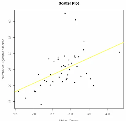
Figure 2.1.3 Scatter plot Number of cigarettes smoked on x (Kidney Cancer)...14 3 Figure 2.1.4 Scatter plot Number of cigarettes smoked on x4(Leukemia)
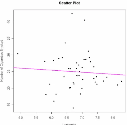
...15
Figure 2.2.1 Partial regression scatter plot..……...16
Figure 2.2.2 (x1*x2) contour plot.……….………..…………..…...16
Figure 2.2.3 Partial regression scatter plot..……...18
Figure 2.2.4 (x1*x3) contour plot………....…………...18
Figure 2.2.5 Partial regression scatter plot..……...20
Figure 2.2.6 (x1*x4) contour plot.………...………....………...20
Figure 2.2.7 Partial regression scatter plot…...…………...………...22
Figure 2.2.8 (x2*x3) contour plot
.………...………...………...22
Figure 2.2.9 Partial regression scatter plot...……....…………...………...24
Figure 2.2.10 (x2*x4) contour plot………..…...24
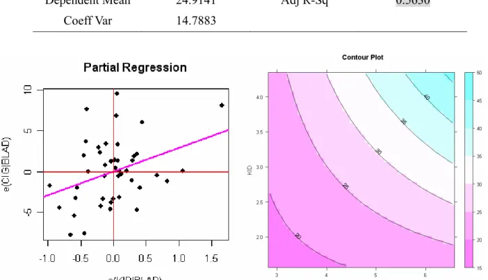
Figure 2.2.11 Partial regression scatter plot…...26
Figure 2.2.12 (x3*x4) contour plot………..…………...26
Figure 2.3.1 Scatterplot matrix for four regressor variables
…….…...28
探討抽菸量與癌症之間關聯性之回歸分析
Figure 3.1.1 Residual Plot for Model 2.3.2
……… 33
Figure 3.1.2 Normal probability plot of residuals for Model 2.3.2
……….33
Figure 3.2.1 Scatterplot matrix for three regressor variables
………38
Figure 3.2.2 Residual Plot for Model 3.2.2
………...…………..39
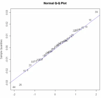
Figure 3.2.3 Normal probability plot of residuals for Model 3.2.2
………...…39
Figure 3.2.4 Influence Index Plot for Model 3.2.2
………42
Figure 3.3.1 The plot of max(lnL(β,σ2,λ))
………..…..45
Figure 3.3.2 Scatterplot matrix for three regressor variables
………..…..45
Figure 3.3.3 Residual Plot for Model 3.3.2
………46
Figure 3.3.4 Normal probability plot of residuals for Model 3.3.2
………47
Figure 3.3.5 Influence Index Plot for Model 3.3.2
……….……50
Figure 3.3.6The plot of max(lnL(β,σ2,λ)) for three regressor
………..…..53
Figure 3.3.7 The plot of max(lnL(β,σ2,λ)) for Response………53
Figure 3.3.8 Scatterplot matrix for three regressor variables
………...….53
Figure 3.4.1 Scatterplot matrix for three regressor variables
………...…….56
Figure 3.4.2 Residual Plot for Model 3.4.2
………56
Figure 3.4.3 Normal probability plot of residuals for Model 3.4.2
………...…..57
Figure 3.4.4 Influence Index Plot for Model 3.4.2
………60
Figure 4.1.1 Plot 2 p R versus p
...………...75
探討抽菸量與癌症之間關聯性之回歸分析
Figure 4.1.3 Plot MSRes(p versus p.………...………...77 )
Figure 4.2.1 Plot 2 p R versus p
...………...84
Figure 4.2.2 The Cp plot
.………..……...85
Figure 4.2.3 Plot MSRes(p versus p.………...………...85 )
Figure 4.3.1 Plot 2 p R versus p
...……….………...91
Figure 4.3.2 The Cp plot
.………..……...91
Figure 4.3.3 Plot MSRes(p versus p.………...………...92 )
Figure 5.1.1 Scatter Plot to Separate the Dummy Variable x4
...93
Figure 5.1.2 Scatter Plot to Separate the Dummy Variable x5
...94
Figure 5.1.3 Scatter Plot to Separate the Dummy Variable x6
...94
Figure 5.1.4 Scatter Plot to Separate the Dummy Variable x5
...95
Figure 5.1.5 Scatter Plot to Separate the Dummy Variable x6
...
....95
Figure 5.1.6 Scatter Plot to Separate the Dummy Variable x5
...96
Figure 5.1.7 Scatter Plot to Separate the Dummy Variable x6
...96
Figure 5.2.1 Response function for Model 5.2.2
……...99
Figure 5.2.2 Normal probability plot of residuals for Model 5.2.2
……...99
Figure 5.2.3 Response function for Model 5.2.5
……...101
Figure 5.2.4 Normal probability plot of residuals for Model 5.2.5
……...102
探討抽菸量與癌症之間關聯性之回歸分析
Figure 5.3.1 Response function for Model 5.3.2
……...106
Figure 5.3.2 Normal probability plot of residuals for Model 5.3.2
……..…...107
Figure 5.3.3 Response function for Model 5.3.5
……...109
Figure 5.3.4 Normal probability plot of residuals for Model 5.3.5
……...109
Figure 5.3.5 Response function for Model 5.3.10
…...111
探討抽菸量與癌症之間關聯性之回歸分析 Ch1 資料介紹 Ch1 統計方法 Ch2 偏回歸 Ch2 複回歸 Ch2 簡單回歸 判斷最佳 模型為何 Ch3 影響點 Ch3 變數轉換 Ch3 平方項加入 殘差分析 判斷最佳 模型為何 Ch4 逐步回歸 判斷最佳 模型為何 Ch5 虛擬變數
研究流程圖
第一章 資料介紹與分析方法陳述
第一節 此組資料為 1960 年蒐集美國 43 州與哥倫比亞特區之已抽香菸頭數(賣出)與每十萬人當 中不同癌症各自之死亡率,其中癌症包含了膀胱癌、肺癌、腎臟癌與白血症,分析癌症與抽 菸之間的關係。而我們參考Fraumeni, J.F. 1968 此篇論文,將地區做細分,分析抽菸與癌症是 否會因地區的不同受環境影響而有所差異。 變數名稱介紹y :已抽過香菸頭數(Number of cigarettes smoked) 1
x :各州每十萬人當中罹患膀胱癌死亡率
(Deaths per 100K population from bladder cancer)
2
x :各州每十萬人當中罹患肺癌死亡率(Deathes per 100K population from lung cancer)
3
x :各州每十萬人當中罹患腎臟癌死亡率(Deaths per 100K population from kidney cancer) 4
x :各州每十萬人當中罹患白血症死亡率(Deaths per 100K population from leukemia)
增加3 個虛擬變數分別為 4 x :菸頭量>平均數23.77 設為 1 菸頭數<平均數 23.77 設為 0 5 x :依地區劃分設 1 為北西部(Northwest) 2 為中西部(Midwest) 3 為南部(South) 4 為西部(West) 6 x :依地區劃分設 1 為南部與西部 0 為北西部與中西部 資料共44 筆與 7 個解釋變數。資料來源:http://lib.stat.cmu.edu Note: 在經過簡單回歸模型配適後發現白血症的死亡率(x4)對菸頭量並無解釋能力,因此在刪 除該解釋變數後加入虛擬變數由x4開始。
44 州分布在美國各地的位置: 虛擬變數中各個值所包含的州 5 x = 1 ⇒ 北西區: 康乃狄克州(CT)、緬因州(ME)、麻薩諸塞州(MA)、新澤西州 (NJ)、紐約 州(NY)、賓夕法尼亞州(PA)、羅德島州(RI)、猶他州(UT)。 2 ⇒ 中西區: 伊利諾州(IL)、印第安納州(IN)、愛荷華州(IO)、堪薩斯州(KS)、密西根 州(MI)、明尼蘇達州(MN)、密蘇里州(MO)、內布拉斯加州(NB)、北達科 他州(ND)、俄亥俄州(OH)、南達科他州(SD)、威斯康辛州(WI)。 3 ⇒ 南區: 阿拉斯加州(AK)、阿拉巴馬州(AL)、阿肯色州(AR)、德拉威州(DE)、哥 倫比亞特區(DC)、佛羅里達州(FL)、肯塔基州(KY)、路易斯安納州(LA)、 馬里蘭州(MD)、密西西比州(MS)、奧克拉荷馬州(OK)、南卡羅來納州 (SC)、田納西州(TE)、德州(TX)、西維吉尼亞州(WV)。 4 ⇒ 西區: 亞利桑那州(AZ)、加州(CA)、愛達荷州(ID)、蒙大拿州(MT)、內華達州 (NE)、新墨西哥州(NM)、猶他州(UT)、華盛頓州(WA)、懷俄明州(WY)。 6 x = 1 ⇒ 南區與西區:阿拉斯加州(AK)、阿拉巴馬州(AL)、阿肯色州(AR)、德拉威州(DE)、 哥倫比亞特區(DC)、佛羅里達州(FL)、肯塔基州(KY)、路易斯安納州 (LA)、馬里蘭州(MD)、密西西比州(MS)、奧克拉荷馬州(OK)、南卡羅 來納州(SC)、田納西州(TE)、德州(TX)、西維吉尼亞州(WV)、亞利桑 那州(AZ)、加州(CA)、愛達荷州(ID)、蒙大拿州(MT)、內華達州(NE)、
0 ⇒ 北西區與中西區:康乃狄克州(CT)、緬因州(ME)、麻薩諸塞州(MA)、新澤西州(NJ)、 紐約州(NY)、賓夕法尼亞州(PA)、羅德島州(RI)、猶他州(UT)、 伊利諾州(IL)、印第安納州(IN)、愛荷華州(IO)、堪薩斯州(KS)、 密西根州(MI)、明尼蘇達州(MN)、密蘇里州(MO)、內布拉斯加 州(NB)、北達科他州(ND)、俄亥俄州(OH)、南達科他州(SD)、 威斯康辛州(WI)。 第二節 我們將利用回歸分析,針對此組資料做探討。而回歸分析(Regression Analysis)是一種 統計分析方法,它利用一組預測變數(或稱獨立變數)的數值,對某一準則變數(或稱應 變數)做預測,它也可以做為評估預測變數對準則變數的影響程度。很不幸地,迴歸 (Regression)的名字取得不理想,從字面上並不能表現出這種方法的重要性及其應用,
取名實際上來自於1885 年高登(Galton)所寫的論文“Regression Toward Mediocrity in Heredity Stature”。大致來說,其意義為:如果一些未知的獨立變數之影響程度消失,
其應變異數應些一迴歸線。迴歸的主要目的是做預測,目標是發展一種能以一個或多
個預測變數的數值來做為應變數預測的方法。迴歸分析就是找出變數間的關係式。我
們將變數分成兩類,一類變數是做為預測提供者,稱為獨立變數(Independent Variable)
或稱為預測變數(Predictor Variable),以x表示,另一類是我們真是關心的被想預測者,
稱為反應變數(Dependent Variable )或準則變數(Response Variable),以 y 表示。
首先,我們針對每個解釋變數膀胱癌(x )、肺癌(1 x )、腎癌(2 x )與白血症(3 x )與反應變數4 菸頭數( y )配適簡單線性回歸模型,依變數解釋能力高低,將所有解釋變數放入模型中並選擇 出最合適的模型。並對模型進行殘差診斷,包含對(1) 預測變數的殘差圖、(2) 配適值的殘差 圖、(3)殘差之常態機率圖。利用VIF診斷預測變數間是否有存在多元共線性存在。若由殘差 圖型發現殘差非固定數或非常態性時,我們可能考慮變數變換等矯正方法。接著使用標準化 後的殘差值來判斷觀測值y 是否存在離群值,和計算帽子矩陣槓桿值判斷觀測值x是否存有 離群值。辨認出離群點後,緊接著探討這些離群值是否具影響力。且我們亦會介紹逐步迴歸
(Stepwise regression),選擇出對回歸模型具有較佳解釋能力之解釋變數之組合。最後,考慮在
模型中加入了虛擬變數x4 = 表菸頭量>平均數 23.77,1 x4 = 表菸頭量<平均數 23.77;依地0
區(AREA)劃分設x5 = 為北西部、1 x5 = 中西部、2 x5 = 南部與3 x5 = 西部;依地區(WEST)劃4
分x6 = 設南部與西部1 x6 = 為北西部與中西部,探討因虛擬變數設定而產生之組別間的差0
第二章 簡單線性回歸分析與複回歸
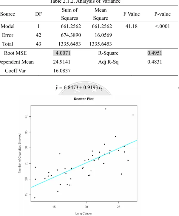
前言 本章首先針對每個解釋變數膀胱癌(x )、肺癌(1 x )、腎癌(2 x )與白血症(3 x )與反應變數菸4 頭數(y )配適簡單線性回歸模型。接著考慮放入兩個解釋變數配進入模型中配適複回歸模型, 而利用偏回歸圖觀察若已有一個解釋變數在模型中,加入另一解釋變數進入模型是否對模型 有幫助,並利用 Contour 圖形觀察解釋變數之間是否有交互作用存在。依序放入三個解釋變 數與四個解釋變數分別配適模型,最後依整體現象選擇出最合適的模型。 第一節 此節為針對每個解釋變數膀胱癌(x )、肺癌(1 x )、腎癌(2 x )與白血症(3 x )與反應變數菸頭4 數(y )配適簡單線性回歸模型。 由 Table 2.1.1-2.1.8 看出x1、x2、x 的 p-value<0.01,參數檢定皆顯著,表示具解釋能力。3 而x4的p-value = 0.6587>0.01,參數不顯著。而相對於其他變數而言,x1的R2 =0.4951為最 大, MSE =4.0071為最小,因此就簡單回歸而言解釋變數x1對y 的解釋能力最高。另外,由 Figure 2.1.4 發現其散佈圖點的散佈情況完全沒有呈現直線的樣子,由x4的R2 =0.0047解釋y 總變異能力僅有0.47%,且 MSE = 5.6260為最大,加上x4的參數檢定並不顯著,因此x4對y 而言可能不具解釋能力。 1 4.064 8.1657 ˆ x y= + (2.1.1)Table 2.1.1. Parameter estimates
Variable DF Parameter Estimate Standard Error t Value P-value
Intercept 1 8.1657 2.6789 3.05 0.0040
1
x 1 4.0640 0.6333 6.42 <.0001
Table 2.1.2. Analysis of Variance
Source DF Sum of
Squares
Mean
Square F Value P-value
Model 1 661.2562 661.2562 41.18 <.0001
Error 42 674.3890 16.0569
Total 43 1335.6453 1335.6453
Root MSE 4.0071 R-Square 0.4951
Dependent Mean 24.9141 Adj R-Sq 0.4831
Coeff Var 16.0837 2 0.9193 6.8473 ˆ x y = + (2.1.2)
Figure 2.1.2: Scatter plot Number of cigarettes smoked on x2(Lung Cancer)
Table 2.1.3. Parameter Estimates
Variable DF Parameter Estimate Standard Error t Value P-value
Table 2.1.4. Analysis of Variance
Source DF Sum of
Squares
Mean
Square F Value P-value
Model 1 649.6181 649.6181 39.77 <.0001
Error 42 686.0271 16.3340
Total 43 1335.6453
Root MSE 4.0415 R-Square 0.4864
Dependent Mean 24.9141 Adj R-Sq 0.4741
Coeff Var 16.2219 3 5.233 10.2902 ˆ x y= + (2.1.3)
Figure 2.1.3: Scatter plot Number of cigarettes smoked on x (Kidney Cancer) 3
Table 2.1.5. Parameter Estimates
Variable DF Parameter Estimate Standard Error t Value P-value
Intercept 1 10.2902 4.1103 2.50 0.0163
Table 2.1.6. Analysis of Variance
Source DF Sum of
Squares Mean Square F Value P-value
Model 1 317.2807 317.2807 13.09 0.0008
Error 42 1018.3646 24.2468
Total 43 1335.6453
Root MSE 4.9241 R-Square 0.2375
Dependent Mean 24.9141 Adj R-Sq 0.2194
Coeff Var 19.7643 4 0.598 28.9982 ˆ x y= − (2.1.4)
Figure 2.1.4: Scatter plot Number of cigarettes smoked on x4(Leukemia)
Table 2.1.7. Parameter Estimates
Variable DF Parameter Estimate Standard Error t Value P-value
Intercept 1 28.9982 9.2200 3.15 0.0030
4
Table 2.1.8. Analysis of Variance
Source DF Sum of
Squares Mean Square F Value P-value
Model 1 6.2638 6.2638 0.2 0.6587
Error 42 1329.3815 31.6519
Total 43 1335.6453
Root MSE 5.6260 R-Square 0.0047
Dependent Mean 24.9141 Adj R-Sq -0.019
Coeff Var 22.5816 第二節 此節為針對解釋變數膀胱癌(x )、肺癌(1 x )、腎癌(2 x )與白血症(3 x ),依序選擇兩個解釋4 變數與反應變數菸頭數(y )配適複回歸模型。並利用偏回歸圖觀察若已有一個解釋變數在模型 中,加入另一解釋變數進入模型是否對模型有幫助,並利用 Contour 圖形觀察解釋變數之間 是否有交互作用存在。
Figure 2.2.1 : Partial regression scatter plot Figure 2.2.2 : (x1*x2) contour plot
2 1 0.5448 2.4922 3.9373 ˆ x x y= + + (2.2.1) 2 1 2 1 0.2761 0.0647 1.1812 9.2118 ˆ x x x x y= + + + (2.2.2) 我們從Figure 2.2.1 的偏回歸圖可看到,在x 已加入模型中的情況下再加入x 後的散佈狀
看出x1與x2的contour plot 並未呈曲線狀,交互作用並不顯著;而由 Table 2.2.1-2.2.4 看出對 1 x 與x2此兩變數而言,未加入交互作用項x1*x2前,x1與x2的p-value<0.01,兩參數估計值皆 為顯著,但加入交互作用項x1*x2後,x1與x2及x1*x2的 p-value>0.01,參數估計值皆變為不 顯著;未加入交互作用項x1*x2前的Radj2 =0.5719較加入後的Radj2 =0.5630來的大,解釋力較 高,而未加入交互作用項x1*x2前的 MSE =3.6465較加入後的 MSE = 3.6844來的小;因此模 型並不適合加入交互作用項x1*x2。
Table 2.2.1. Parameter Estimates
Variable DF Parameter Estimate Standard Error t Value P-value
Intercept 1 3.9373 2.7898 1.41 0.1657
1
x 1 2.4922 0.7658 3.25 0.0023
2
x 1 0.5448 0.1748 3.12 0.0033
Table 2.2.2. Analysis of Variance
Source DF Sum of
Squares
Mean
Square F Value P-value
Model 2 790.4571 395.2285 29.72 <.0001
Error 41 545.1882 13.2973
Total 43 1335.6453
Root MSE 3.6465 R-Square 0.5918
Dependent Mean 24.9141 Adj R-Sq 0.5719
Coeff Var 14.6365
Table 2.2.3. Parameter Estimates
Variable DF Parameter Estimate Standard Error t Value P-value
Intercept 1 9.2118 13.3850 0.69 0.4953 1 x 1 1.1812 3.3430 0.35 0.7257 2 x 1 0.2761 0.6895 0.40 0.6910 1 x *x2 1 0.0647 0.1605 0.40 0.6890
Table 2.2.4. Analysis of Variance
Source DF Sum of
Squares
Mean
Square F Value P-value
Model 3 792.6628 264.2209 19.46 <.0001
Error 40 542.9825 13.5746
Total 43 1335.6453
Root MSE 3.6844 R-Square 0.5935
Dependent Mean 24.9141 Adj R-Sq 0.5630
Coeff Var 14.7883
Figure 2.2.3 : Partial regression scatter plot Figure 2.2.4 : (x1*x3) contour plot
3 1 2.895 3.5052 2.3783 ˆ x x y= + + (2.2.3) 3 1 3 1 3.7462 1.8918 1.8944 21.0707 ˆ x x x x y= − − + (2.2.4) 我們從Figure 2.2.3 的偏回歸圖可看到,在x1已加入模型中的情況下再加入x 後的散佈狀3 況大致呈一直線,表示模型在x1解釋完後,x 的加入對模型依舊有解釋能力。由 Figure 2.2.43
看出x1與x 的 contour plot 雖稍微呈曲線狀,但交互作用仍未達顯著的標準;由 Table 2.2.5-3
2.2.8 看出對x1與x 此兩變數而言,加入交互作用項3 x1*x 後的3 2 0.5402 adj R = 雖然較加入前 2 0.5369 adj R = 來的大,解釋力較高,而加入交互作用項x1*x 後的3 MSE = 3.7794也較加入前的 3.7928 MSE = 來的小;但未加入交互作用項x *x 前,x 與x 的 p-value<0.01,兩參數估計值
不顯著;因此模型並不適合加入交互作用項x1*x3。
Table 2.2.5. Parameter Estimates
Variable DF Parameter Estimate Standard Error t Value P-value
Intercept 1 2.3783 3.4820 0.68 0.4984
1
x 1 3.5052 0.6422 5.46 <0.0001
3
x 1 2.8950 1.1938 2.43 0.0198
Table 2.2.6. Analysis of Variance
Source DF Sum of
Squares Mean Square F Value P-value
Model 2 745.8597 372.9298 25.92 <.0001
Error 41 589.7856 14.3850
Total 43 1335.6453
Root MSE 3.7928 R-Square 0.5584
Dependent Mean 24.9141 Adj R-Sq 0.5369
Coeff Var 15.2234
Table 2.2.7. Parameter Estimates
Variable DF Parameter Estimate Standard Error t Value P-value
Intercept 1 21.0707 16.8103 1.25 0.2173 1 x 1 -1.8944 4.7943 -0.40 0.6948 3 x 1 -3.7462 5.9678 -0.63 0.5335 1 x *x 3 1 1.8918 1.6647 1.14 0.2625
Table 2.2.8. Analysis of Variance
Source DF Sum of
Squares Mean Square F Value P-value
Model 3 764.3063 254.7688 17.84 <.0001
Error 40 571.3389 14.2835
Total 43 1335.6453
Root MSE 3.7794 R-Square 0.5722
Dependent Mean 24.9141 Adj R-Sq 0.5402
Figure 2.2.5 : Partial regression scatter plot Figure 2.2.6 : (x1*x4) contour plot (2.2.5) 4.2397 4.2397 18.6245 ˆ x1 x4 y= + − (2.2.6) 1.1722 2.668 12.2147 10.5373 ˆ x1 x4 x1x4 y=− + + − 我們從Figure 2.2.5 的偏回歸圖可看到,在x1已加入模型中的情況下再加入x4後的散佈狀 況較似隨機分佈,並不呈一直線,表示模型在x1解釋完後,x4的加入對模型並無解釋能力。
由Figure 2.2.6 看出x1與x4的contour plot 曲線狀並不明顯,交互作用不顯著;而由 Table 2.2.9 -2.2.12 看出對x1與x4此兩變數而言,未加入交互作用項x1*x4前,x1的p-value<0.01,而x4 的p-value>0.01,x1的參數估計值為顯著,x4的參數估計值不顯著,但加入交互作用項x1*x4 後,x1與x4及x1*x4的 p-value>0.01,參數估計值皆變為不顯著;未加入交互作用項x1*x4前 的Radj2 =0.5064較加入後的Radj2 =0.5006來的大,解釋力較高,而未加入交互作用項x1*x4前 的 MSE =3.9158較加入後的 MSE = 3.9387來的小;因此模型並不適合加入變數x4及交互作用 項x1*x4。
Table 2.2.9. Parameter Estimates
Variable DF Parameter Estimate Standard Error t Value P-value
Intercept 1 18.6245 6.5980 2.82 0.0073
1
x 1 4.2397 0.6272 6.76 <0.0001
4
Table 2.2.10. Analysis of Variance
Source DF Sum of
Squares Mean Square F Value P-value
Model 2 706.9820 353.4910 23.05 <.0001
Error 41 628.6632 15.3333
Total 43 1335.6453
Root MSE 3.9158 R-Square 0.5293
Dependent Mean 24.9141 Adj R-Sq 0.5064
Coeff Var 15.7171
Table 2.2.11. Parameter Estimates
Variable DF Parameter Estimate Standard Error t Value P-value
Intercept 1 -10.5373 40.7896 -0.26 0.7975 1 x 1 12.2147 11.0244 1.11 0.2745 4 x 1 2.6680 6.0178 0.44 0.6599 1 x *x4 1 -1.1722 1.6178 -0.72 0.4729
Table 2.2.12. Analysis of Variance
Source DF Sum of
Squares Mean Square F Value P-value
Model 3 715.1268 238.3756 15.37 <.0001
Error 40 620.5185 15.5130
Total 43 1335.6453
Root MSE 3.9387 R-Square 0.5354
Dependent Mean 24.9141 Adj R-Sq 0.5006
Figure 2.2.7 : Partial regression scatter plot Figure 2.2.8 : (x2*x3) contour plot
yˆ =−0.3064+0.8017x2 +3.3866x3 (2.2.7) yˆ =−2.1452+0.8998x2 +4.0175x3 −0.0333x2x3 (2.2.8)
我們從Figure 2.2.7 的偏回歸圖可看到,在x2已加入模型中的情況下再加入x 後的散佈狀3
況大致呈一直線,表示模型在x2解釋完後,x 的加入對模型依舊有解釋能力。由 Figure 2.2.83
看出x2與x 的 contour plot 並未呈曲線狀,交互作用並不顯著;而由 Table 2.2.13-2.2.16 看出3
對x2與x 此兩變數而言,未加入交互作用項3 x2*x 前,3 x2與x 的 p-value<0.01,兩參數估計3 值皆為顯著,但加入交互作用項x2*x 後,3 x2與x 及3 x2*x 的 p-value>0.01,參數估計值皆變3 為不顯著;未加入交互作用項x2*x 前的3 2 0.5573 adj R = 較加入後的Radj2 =0.5465來的大,解釋 力較高,而未加入交互作用項x2*x 前的3 MSE = 3.7082較加入後的 MSE = 3.7534來的小;因 此模型並不適合加入交互作用項x2*x3。
Table 2.2.13. Parameter Estimates
Variable DF Parameter Estimate Standard Error t Value P-value
Intercept 1 -0.3064 3.6024 -0.09 0.9326
2
x 1 0.8017 0.1394 5.75 <0.0001
3
Table 2.2.14. Analysis of Variance
Source DF Sum of
Squares
Mean
Square F Value P-value
Model 2 771.8778 385.9389 28.07 <.0001
Error 41 563.7675 13.7504
Total 43 1335.6453
Root MSE 3.7082 R-Square 0.5779
Dependent Mean 24.9141 Adj R-Sq 0.5573
Coeff Var 14.8838
Table 2.2.15. Parameter Estimates
Variable DF Parameter Estimate Standard Error t Value P-value
Intercept 1 -2.1452 14.2827 -0.15 0.8814 2 x 1 0.8998 0.7499 1.20 0.2372 3 x 1 4.0175 4.8751 0.82 0.4148 2 x *x 3 1 -0.0333 0.2504 -0.13 0.8947
Table 2.2.16. Analysis of Variance
Source DF Sum of
Squares
Mean
Square F Value P-value
Model 3 772.1276 257.3759 18.27 <.0001
Error 40 563.5177 14.0879
Total 43 1335.6453
Root MSE 3.7534 R-Square 0.5781
Dependent Mean 24.9141 Adj R-Sq 0.5465
Figure 2.2.9 : Partial regression scatter plot Figure 2.2.10 : (x2*x4) contour plot (2.2.10) 0.0889 2.0189 1.5311 7.0722 ˆ (2.2.9) 0.3328 0.9269 4.4249 ˆ 4 2 4 2 4 2 x x x x y x x y − + + − = + + = 我們從 Figure 2.2.9 的偏回歸圖可看到,在x2已加入模型中的情況下再加入x4後的散佈 狀況較似隨機分佈,並不呈一直線,表示模型在x2解釋完後,x4的加入對模型並無解釋能力。
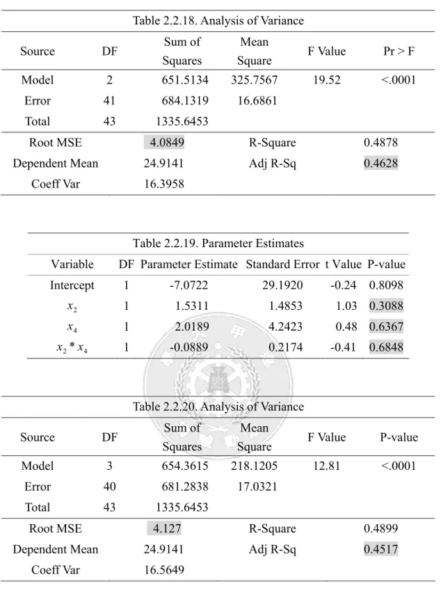
由Figure 2.2.10 看出x2與x4的contour plot 未呈曲線狀,交互作用不顯著;而由 Table 2.2.17 -2.2.20 看出對x2與x4此兩變數而言,未加入交互作用項x2*x4前,x2的p-value<0.01,而x4 的p-value>0.01,x2的參數估計值為顯著,x4的參數估計值不顯著,但加入交互作用項x2*x4 後,x2與x4及x2*x4的p-value>0.01,參數估計值皆變為不顯著;未加入交互作用項x2*x4前 的 2 0.4628 adj R = 較加入後的 2 0.4517 adj R = 來的大,解釋力較高,而未加入交互作用項x2*x4前的 4.0849 MSE = 較加入後的 MSE = 4.127來的小;因此模型並不適合加入變數x4及交互作用項 2 x *x4。
Table 2.2.17. Parameter Estimates
Variable DF Parameter Estimate Standard Error t Value P-value Intercept 1 4.4249 7.7735 0.57 0.5723
2
x 1 0.9269 0.1491 6.22 <0.0001
4
Table 2.2.18. Analysis of Variance Source DF Sum of Squares Mean Square F Value Pr > F Model 2 651.5134 325.7567 19.52 <.0001 Error 41 684.1319 16.6861 Total 43 1335.6453
Root MSE 4.0849 R-Square 0.4878
Dependent Mean 24.9141 Adj R-Sq 0.4628
Coeff Var 16.3958
Table 2.2.19. Parameter Estimates
Variable DF Parameter Estimate Standard Error t Value P-value
Intercept 1 -7.0722 29.1920 -0.24 0.8098 2 x 1 1.5311 1.4853 1.03 0.3088 4 x 1 2.0189 4.2423 0.48 0.6367 2 x *x4 1 -0.0889 0.2174 -0.41 0.6848
Table 2.2.20. Analysis of Variance
Source DF Sum of
Squares
Mean
Square F Value P-value
Model 3 654.3615 218.1205 12.81 <.0001
Error 40 681.2838 17.0321
Total 43 1335.6453
Root MSE 4.127 R-Square 0.4899
Dependent Mean 24.9141 Adj R-Sq 0.4517
Figure 2.2.11 : Partial regression scatter plot Figure 2.2.12 : (x3*x4) contour plot (2.2.11) 1.4529 5.5702 19.2708 ˆ x3 x4 y= + − 4 3 4 3 3.8297 3.8297 3.8297 24.9447 ˆ x x x x y= + − + (2.2.12) 我們從Figure 2.2.11 的偏回歸圖可看到,在x 已加入模型中的情況下再加入3 x4後的散佈 狀況較似隨機分佈,並不呈一直線,表示模型在x 解釋完後,3 x4的加入對模型並無解釋能力。
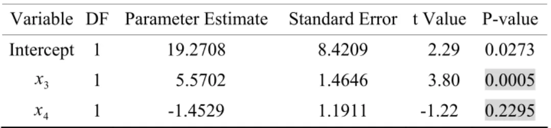
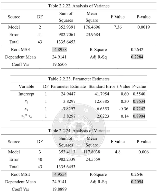
由Figure 2.2.12 看出x 與3 x4的contour plot 未呈曲線狀,交互作用不顯著;而由 Table 29-32 看出對x 與3 x4此兩變數而言,未加入交互作用項x *3 x4前,x 的 p-value<0.01,而3 x4的 p-value>0.01,x 的參數估計值為顯著,3 x4的參數估計值不顯著,但加入交互作用項x *3 x4後, 3 x 與x4及x *3 x4的 p-value>0.01,參數估計值皆變為不顯著;未加入交互作用項x *3 x4前的 2 0.2284 adj R = 較加入後的Radj2 =0.2094來的大,解釋力較高,而未加入交互作用項x *3 x4前的 4.8958 MSE = 較加入後的 MSE =4.9554來的小;因此模型並不適合加入變數x4及交互作用項 3 x *x4。
Table 2.2.21. Parameter Estimates
Variable DF Parameter Estimate Standard Error t Value P-value
Intercept 1 19.2708 8.4209 2.29 0.0273
3
x 1 5.5702 1.4646 3.80 0.0005
4
Table 2.2.22. Analysis of Variance
Source DF Sum of
Squares
Mean
Square F Value P-value
Model 2 352.9391 176.4696 7.36 0.0019
Error 41 982.7061 23.9684
Total 43 1335.6453
Root MSE 4.8958 R-Square 0.2642
Dependent Mean 24.9141 Adj R-Sq 0.2284
Coeff Var 19.6506
Table 2.2.23. Parameter Estimates
Variable DF Parameter Estimate Standard Error t Value P-value
Intercept 1 24.9447 41.7954 0.60 0.5540 3 x 1 3.8297 12.6385 0.30 0.7634 4 x 1 -3.8297 6.6353 -0.36 0.7242 3 x *x4 1 3.8297 2.0223 0.14 0.8904
Table 2.2.24. Analysis of Variance
Source DF Sum of
Squares
Mean
Square F Value P-value
Model 3 353.4113 117.8038 4.8 0.006
Error 40 982.2339 24.5559
Total 43 1335.6453
Root MSE 4.9554 R-Square 0.2646
Dependent Mean 24.9141 Adj R-Sq 0.2094
Coeff Var 19.8899 第三節 由前兩節所配適的簡單線性回歸,發現解釋變數白血症(x )放入模型中解釋能力似乎較4 為低。而在兩兩變數的模型中,我們發現偏回歸圖,在考慮白血症(x )加入模型的情形,其4 偏回歸圖形幾乎呈水平線, 表示白血症(x )加入模型中似乎並無幫助。而本節我們先利用相4 關係數矩陣觀察變數之間的關係,並比較將所有解釋變數放入模型中與只放三個解釋變數膀 胱癌(x )、肺癌(x )、腎癌(x )與反應變數菸頭數( y )的情況,並選擇較適當的模型。
Figure 2.3.1 : Scatterplot matrix for four regressor variables 4 3 2 1 0.433 2.9272 1.1954 2.378 6.5897 ˆ x x x x y = + + + − (2.3.1) 我們由 Figure 2.3.2 大概發現x4與y 的相關係數散佈幾乎接近圓形,可看出x4與y 的相 關性非常低;而x1對y 以及x2對y 的相關係數散佈較接近一直線,可看出x1、x2與y 的相關 性較高;而x 對 y 的相關性則僅次於3 x1與x2。而從Table 2.3.1 的相關係數矩陣亦可看出此現 象 , 相 較 於 其 他 變 數 而 言 0.7036 1 ,x = y r 呈 現 高 度 正 相 關 , 可 知x1與 y 有線性關係;而 -0.0685 4 ,x = y r 呈現低度負相關,x4與y 之線性關係最低。 而由Table 2.3.2 我們可以發現 將四個解釋變數均放入的模型,除了x4的p-value>0.01 參數值 不顯著外,其他三個變數p-value 皆大於 0.01,參數值均顯著,在模型均具解釋能力。因此, 我們判斷x4也許應該從模型中剔除。
Table 2.3.1. correlation coefficient matrix y x1 x2 x 3 x4 y 1 0.7036 0.6974 0.4874 -0.0685 1 x 0.7036 1 0.6585 0.3588 0.1622 2 x 0.6974 0.6585 1 0.2827 -0.1516 3 x 0.4874 0.3588 0.2827 1 0.1887 4 x -0.0685 0.1622 -0.1516 0.1887 1
Table 2.3.2. Parameter Estimates
Variable DF Parameter Estimate Standard Error t Value P-value
Intercept 1 6.5897 6.7021 0.98 0.3316 1 x 1 2.3780 0.7756 3.07 0.0039 2 x 1 0.4330 0.1755 2.47 0.0181 3 x 1 2.9272 1.0919 2.68 0.0107 4 x 1 -1.1954 0.8940 -1.34 0.1889
Table 2.3.3. Analysis of Variance
Source DF Sum of
Squares
Mean
Square F Value P-value
Model 4 882.8688 220.7172 19.01 <.0001
Error 39 452.7765 11.6097
Total 43 1335.6453
Root MSE 3.4073 R-Square 0.661
Dependent Mean 24.9141 Adj R-Sq 0.6262
Figure 2.3.3 : Scatterplot matrix for three regressor variables 3 2 1 0.5179 2.6701 2.0544 1.1916 ˆ x x x y=− + + + (2.3.2) 由 Table 2.3.4 我們可以看到,剔除解釋變數x4後的模型,參數值均為顯著,且其 2 0.6189 Adj R = 。與模型2.3.1 之 2 0.6262 Adj R = 相較下,其解釋總變異能力只降低0.73%。近一步 觀察解釋變數之間的相關性,由 1 VIFx 、 2 VIFx 、VIFx3均接近1 小於 10,表示這三個變數並無 強烈的多元共線性問題存在。
Table 2.3.4. Parameter Estimates
Variable DF Parameter Estimate Standard Error t Value P-value Variance Inflation
Intercept 1 -1.1916 3.3579 -0.35 0.7246 0 1 x 1 2.0544 0.7441 2.76 0.0087 1.8727 2 x 1 0.5179 0.1653 3.13 0.0032 1.7734 3 x 1 2.6701 1.0853 2.46 0.0183 1.1528
Table 2.3.5. Analysis of Variance
Source DF Sum of
Squares
Mean
Square F Value P-value
Model 4 0.0184 0.0184 127.0766 0.0013
Error 39 0.0056 0.0001
Total 43 0.0240
第四節 綜合以上結果,我們可以看到,無論是單一解釋變數的簡單線性回歸模式、兩解釋變數 的複模式、討論加入交互作用項的兩解釋變數的複回歸模式及四個解釋變數均加入的回歸模 式,解釋變數x4在模型中的參數檢定均不顯著。而由相關係數矩陣與圖形也可發現,x4與y 的線性關係度很低。因此,我們判斷解釋變數x4應從模型中踢除。我們認為模型 2.3.2 為最 佳模型,下一章我們將對模型2.3.2 進行殘差分析診斷。
第三章 模型之診斷及矯正策略
前言 本章主要是針對模型進行殘差診斷,包含對(1) 預測變數的殘差圖、(2) 配適值的殘差 圖、(3)殘差之常態機率圖。利用VIF診斷預測變數間是否有存在多元共線性存在。若由殘差 圖型發現殘差非固定數或非常態性時,我們可能考慮變數變換等矯正方法。接著使用標準化 後的殘差值來判斷觀測值y 是否存在離群值,和計算帽子矩陣槓桿值判斷觀測值x是否存有 離群值。辨認出離群點後,緊接著探討這些離群值是否具影響力。使用Cook’s D 判斷其對所 有配適值之影響、而DFFITSi為判斷其對單一配適值之影響與DFBETASji為用於判斷其對迴歸 係數之影響。COVRATIOi >1時,表示觀察值i 可以改善估計精確度;COVRATIOi < 時,表示1 觀察值i 降低估計精確度,COVRATIOi > +1 3 /p n or COVRATIOi <1- 3 /p n 則第 i 筆觀察值可 能為影響點。最後,因我們知道最小平方法容易受影響點影響,嚴重時可能會扭曲其餘觀測 值之配適情形。也可能會導致遺漏重要的變數或選用不正確的函數形式。所以我們可能會比 較其與刪去影響點之後配模的差別。 第一節 根據第二章結果所選擇之最佳模型2.3.2 進行模型之診斷,包含殘差圖形診斷、判斷離群 值與影響點等分析。從Figure 3.1.1 模型 2.3.2 之殘差圖(a)發現殘差變異數不一致且略呈曲 線,殘差圖(b)(c)(d)殘差點的散佈亦無在 0 上下均勻散佈,且均呈現有離群值存在的現象。而 由Figure 3.1.2 殘差機率圖發現明顯觀察出離群值且為輕尾分佈(Light – tailed errors)。接下來 我們利用數值方法判斷是否有離群值與影響點存在。Figure 3.1.1: Residual Plot for Model 2.3.2
離群值分析(n = 44, p = 4) 1. 對x之影響 利用 hat matrix 之對角線來檢視x之離群值,因h 表示每個解釋變數之元素與各解釋變數ii 平均之距離量度,而判別式為: h hii >2 , n p h = , 計算結果臨界值為 0.1818,由 Table3.2.1 可以得知,在此條件下符合的觀察值有第 1、 26、 30、33 等四筆。 2. 對 y 之影響 利用d 、i t 來判斷i y 之離群值,其判別式為: e 3 = i > i R s e d MS ⇒ >ei 3 MSR se / 2 , 1 i n n p t >tα − − 由 Table 3.1.1 顯示,其中d 大於i 3 MSE=10.32 的只有第 26 筆資料,而在t0.0011,39 = 3.5134 條件下,沒有任何資料大於臨界值但第26 筆ti = 3.4785 接近此值,因此結果為第 26 筆觀察 值可能為y 之影響點。 3. 對 ˆy 之影響 為考慮第 i 筆觀察值對所有配適值之影響,為一比較综合影響之量數,其意涵在於檢測第 i 筆是否為影響全體配適值結果之影響點,其判別式為: Cook’s D> 1F0.5,p,n− p ≈ 由 Table 3.1.1 結果顯示沒有任何一筆Cook’s D 值大於 1,只有在第 26 筆資料是 0.8172 最接近1,因此考慮第 26 筆為影響點。 4. 對 ˆy 之影響 i 計算由全體配適值減去捨棄第i 筆所估計配適值之差除以全體之標準差估計值,其涵義為 加入第i 筆觀察值導致配適值增減多少倍的標準差估計值,其判別式為: 2 i p DFFITS > n 由 Table 3.1.2 結果顯示在臨界值 2 p n = 0.603 下符合的觀察值有第 8、16、26 等三筆可
5. 對回歸係數( ˆβ’s)之影響 ji DFBETAS 其涵義本身指出納入一個觀察值將導致估計的回歸係數會增大或減少,此絕對 量顯示相對於此回歸係數之估計的標準誤其差異量大小,大的DFBETASji值直接表示第i 筆觀 察質對第 j 個回歸係數具有較大的衝擊,因此作為辨認影響點的依據,其判別式為: , 2 / j i DFBETAS > n, 其臨界值為0.3015,由Table 3.1.2 結果顯示第 26 筆資料對所有回歸係數而言有明顯的效果; 而個別對於β 而言第 8、26 這兩筆符合判斷標準,對於ˆ0 βˆ1而言第26、42 這兩筆符合判斷標 準,對於βˆ2而言第8、26 這兩筆符合判斷標準,對於βˆ3而言第26、42 這兩筆符合判斷標準。 其中βˆ0最大影響力都出現在第8 筆資料,而βˆ1、βˆ2、βˆ3最大影響力都出現在第26 筆資料。 6. 對精確度之影響 主要顯示出去除某一筆觀測值後與全體之變異數之比例,COVRATIOi >1時,表示加入第 i 筆觀察值可以改善估計精確度;COVRATIOi < 時,表示加入第i 筆觀察值降低估計精確度,1
一般來說其臨界值難以估計,因此我們參考Belsley, kuh, and welsch [1980]所提供的結果,其
判別式如下: 1 3 1 3 p n COVRATIO p n ⎧> + ⎪⎪ ⎨ ⎪< − ⎪⎩ 其臨界值應大於1.2727或小於0.7273,由Table 3.1.2 結果顯示第 1、2、30、33 這四筆觀察值 可以改善估計精確度,而第8、26、44 這三筆觀察值則會降低估計的精確度。 綜合以上判斷標準可以確定第 26 筆觀察值為影響點,而第 8 筆觀察值則需要我們多加 注意其可能為影響點。
Table 3.1.1: Residual analysis
Obs y ˆy ei Ri Ti hii PRESS COOK’s D Obs y ˆy ei Ri Ti hii PRESS COOK’s D 1 30.34 30.8536 -0.5136 -0.1979 -0.1955 0.4312 -0.9029 0.0074 23 27.56 24.7816 2.7784 0.8218 0.8184 0.0344 2.8776 0.0060 2 18.20 17.8411 0.3589 0.1136 0.1122 0.1571 0.4258 0.0006 24 23.75 26.1799 -2.4299 -0.7314 -0.7271 0.0677 -2.6064 0.0097 3 25.82 23.6362 2.1838 0.6478 0.6431 0.0402 2.2752 0.0044 25 23.32 22.8956 0.4244 0.1258 0.1243 0.0390 0.4416 0.0002 4 18.24 18.6200 -0.3800 -0.1155 -0.1141 0.0854 -0.4155 0.0003 26 42.40 31.7802 10.6198 3.4785 4.1127 0.2127 13.4886 0.8172 5 28.60 26.5026 2.0974 0.6205 0.6157 0.0349 2.1733 0.0035 27 28.64 32.8628 -4.2228 -1.3018 -1.3136 0.1112 -4.7512 0.0530 6 31.10 30.0739 1.0261 0.3077 0.3042 0.0604 1.0921 0.0015 28 21.16 19.0503 2.1097 0.6343 0.6295 0.0655 2.2575 0.0071 7 33.60 30.3133 3.2867 0.9909 0.9907 0.0708 3.5369 0.0187 29 29.14 30.9308 -1.7908 -0.5387 -0.5339 0.0667 -1.9187 0.0052 8 40.46 32.7924 7.6676 2.3532 2.5033 0.1032 8.5495 0.1592 30 19.96 20.6877 -0.7277 -0.2392 -0.2364 0.2181 -0.9307 0.0040 9 28.27 26.6118 1.6582 0.4993 0.4945 0.0683 1.7797 0.0046 31 26.38 27.2042 -0.8242 -0.2432 -0.2403 0.0298 -0.8496 0.0005 10 20.10 18.7369 1.3631 0.4114 0.4071 0.0725 1.4697 0.0033 32 23.44 21.4418 1.9982 0.6069 0.6020 0.0843 2.1822 0.0085 11 27.91 28.2507 -0.3407 -0.1009 -0.0996 0.0367 -0.3537 0.0001 33 23.78 22.4684 1.3116 0.4423 0.4378 0.2573 1.7659 0.0169 12 26.18 25.2264 0.9536 0.2806 0.2773 0.0240 0.9771 0.0005 34 29.18 28.9058 0.2742 0.0817 0.0807 0.0488 0.2883 0.0001 13 22.12 23.8330 -1.7130 -0.5110 -0.5062 0.0506 -1.8043 0.0035 35 18.06 19.9955 -1.9355 -0.5850 -0.5801 0.0753 -2.0932 0.0070 14 21.84 21.1973 0.6427 0.1937 0.1914 0.0701 0.6912 0.0007 36 20.94 21.8973 -0.9573 -0.2914 -0.2881 0.0883 -1.0501 0.0021 15 23.44 19.5425 3.8975 1.1863 1.1925 0.0882 4.2743 0.0340 37 20.08 19.7834 0.2966 0.0898 0.0886 0.0777 0.3216 0.0002 16 21.58 27.6821 -6.1021 -1.8824 -1.9469 0.1123 -6.8741 0.1121 38 22.57 23.3259 -0.7559 -0.2285 -0.2258 0.0753 -0.8175 0.0011 17 28.92 28.0906 0.8294 0.2465 0.2436 0.0440 0.8676 0.0007 39 14.00 17.7021 -3.7021 -1.1460 -1.1506 0.1185 -4.1996 0.0441 18 25.91 30.8345 -4.9245 -1.4980 -1.5225 0.0872 -5.3948 0.0536 40 25.89 27.7734 -1.8834 -0.5578 -0.5529 0.0368 -1.9554 0.0030 19 26.92 27.9475 -1.0275 -0.3038 -0.3003 0.0335 -1.0631 0.0008 41 21.17 25.0642 -3.8942 -1.1462 -1.1508 0.0249 -3.9935 0.0084 20 24.96 29.3310 -4.3710 -1.3075 -1.3196 0.0560 -4.6304 0.0254 42 21.25 26.2580 -5.0080 -1.5324 -1.5596 0.0978 -5.5510 0.0637 21 22.06 23.2564 -1.1964 -0.3758 -0.3717 0.1438 -1.3973 0.0059 43 22.86 25.4286 -2.5686 -0.8024 -0.7988 0.1344 -2.9674 0.0250
Table 3.1.2:Diagnostics for Leverage and Influence
ji
DFBETAS DFBETASji
Obs ei Ti hii COVRATIOi DFFITSi β0 β1 β2 β3 Obs ei Ti hii COVRATIOi DFFITSi β0 β1 β2 β3
1 -0.5136 -0.1955 0.4312 1.9380 -0.1703 0.0942 0.1151 -0.0924 -0.1285 23 2.7784 0.8184 0.0344 1.0706 0.1546 0.0427 -0.0323 0.0664 -0.0643 2 0.3589 0.1122 0.1571 1.3111 0.0484 0.0399 -0.0117 0.0079 -0.0377 24 -2.4299 -0.7271 0.0677 1.1247 -0.1960 0.0716 0.0605 -0.0018 -0.1580 3 2.1838 0.6431 0.0402 1.1052 0.1315 0.0276 -0.0860 0.0583 0.0109 25 0.4244 0.1243 0.0390 1.1497 0.0250 0.0070 -0.0010 -0.0115 0.0088 4 -0.3800 -0.1140 0.0854 1.2083 -0.0348 -0.0308 0.0091 0.0010 0.0208 26 10.6198 4.1127 0.2127 0.3327 2.1375 -0.4290 1.9376 -0.7622 -0.5485 5 2.0974 0.6157 0.0349 1.1031 0.1171 0.0020 0.0070 0.0459 -0.0424 27 -4.2228 -1.3136 0.1112 1.0471 -0.4647 0.2528 -0.2638 -0.0634 0.0188 6 1.0261 0.3042 0.0604 1.1666 0.0771 -0.0495 0.0242 0.0025 0.0358 28 2.1097 0.6295 0.0655 1.1372 0.1666 0.1203 -0.0600 -0.0476 -0.0048 7 3.2867 0.9907 0.0708 1.0781 0.2734 -0.1859 -0.0478 0.1385 0.1323 29 -1.7908 -0.5339 0.0666 1.1516 -0.1427 0.0820 -0.0395 -0.0513 -0.0101 8 7.6676 2.5033 0.1032 0.6799 0.8490 -0.52090.1769 0.4225 0.0136 30 -0.7277 -0.2364 0.2181 1.4071 -0.1248 -0.0026 0.0276 0.0570 -0.0930 9 1.6582 0.4945 0.0683 1.1584 0.1339 0.0142 -0.0076 0.0771 -0.0775 31 -0.8242 -0.2403 0.0298 1.1339 -0.0421 0.0124 0.0008 -0.0140 -0.0058 10 1.3631 0.4071 0.0725 1.1730 0.1138 0.0885 -0.0078 -0.0611 -0.0137 32 1.9982 0.6020 0.0843 1.1646 0.1827 0.0747 -0.1419 0.0992 -0.0292 11 -0.3407 -0.0996 0.0367 1.1476 -0.0195 0.0073 -0.0031 -0.0064 -0.0007 33 1.3116 0.4378 0.2573 1.4609 0.2577 0.0706 0.2007 -0.2361 -0.0152 12 0.9536 0.2773 0.0240 1.1249 0.0435 0.0029 -0.0076 0.0098 0.0012 34 0.2742 0.0807 0.0488 1.1625 0.0183 -0.0057 0.0053 0.0063 -0.0036 13 -1.7130 -0.5062 0.0506 1.1354 -0.1169 -0.0261 -0.0557 0.0852 -0.0194 35 -1.9355 -0.5801 0.0753 1.1563 -0.1656 -0.1345 0.0401 -0.0162 0.1103 14 0.6427 0.1914 0.0701 1.1856 0.0526 0.0154 -0.0366 0.0052 0.0196 36 -0.9573 -0.2880 0.0883 1.2035 -0.0897 -0.0186 -0.0114 0.0628 -0.0428 15 3.8975 1.1925 0.0882 1.0516 0.3708 0.2637 -0.2055 0.1127 -0.1726 37 0.2966 0.0886 0.0777 1.1989 0.0257 0.0186 -0.0136 0.0068 -0.0117 16 -6.1021 -1.9469 0.1123 0.8602 -0.6925 -0.0305 0.0445 -0.4496 0.4169 38 -0.7559 -0.2257 0.0753 1.1904 -0.0644 -0.0105 0.0520 -0.0415 -0.0025 17 0.8294 0.2436 0.0440 1.1505 0.0523 -0.0236 0.0185 -0.0092 0.0238 39 -3.7021 -1.1506 0.1185 1.0984 -0.4218 -0.3444 -0.1199 0.3009 0.1487 18 -4.9245 -1.5225 0.0872 0.9623 -0.4706 0.1933 -0.0435 -0.2872 0.0964 40 -1.8834 -0.5529 0.0368 1.1135 -0.1081 0.0486 -0.0197 0.0006 -0.0491 19 -1.0275 -0.3003 0.0335 1.1344 -0.0559 0.0224 -0.0104 -0.0101 -0.0114 41 -3.8942 -1.1508 0.0248 0.9929 -0.1837 -0.0194 0.0431 -0.0515 0.0030 20 -4.3710 -1.3196 0.0560 0.9843 -0.3215 0.1151 -0.1950 0.0149 0.0188 42 -5.0080 -1.5596 0.0978 0.9629 -0.5135 -0.1259-0.37410.1388 0.3266 21 -1.1964 -0.3717 0.1438 1.2742 -0.1523 0.0103 -0.0080 0.0898 -0.1098 43 -2.5686 -0.7988 0.1344 1.1980 -0.3147 0.0156 -0.1967 0.2548 -0.1135
第二節
因我們知道最小平方法容易受影響點影響,嚴重時可能會扭曲其餘觀測值之配適情形。 也可能會導致遺漏重要的變數或選用不正確的函數形式。故我們將由第一節離群值分析所得
到的第8 筆觀察值和第 26 筆觀察值兩個影響點刪去,比較在刪去影響點後之差異,且我們亦
可觀察在少了此兩筆影響點下,模型之配適情形。
Figure 3.2.1: Scatterplot matrix for three regressor variables
在刪去第26 筆及第 8 筆觀察值後,令模型為: =β +β +β +β *+ε 3 3 * 2 2 * 1 1 0 * x x x y (3.2.1) Figure 3.2.1 為刪去兩個影響點後所有變數的多重散佈圖,比較轉換前 Figure2.3.3 多重 散佈圖我們可以明顯的發現y 成鐘形散佈,以模型 3.2.1 作模型參數估計及殘差分析,結果* 從Table 3.2.1 可以看到此參數估計式為: * 3 * 2 * 1 * 2.0274 0.5962 0.5567 3.1969 ˆ x x x y = + + + (3.2.2) 並發現在α =0.05下常數項和解釋變數膀胱癌( * 1 x )的參數檢定卻不顯著,而由 Table 3.2.2 可看出R = 68.10%,2 2 adj R = 65.58%顯示在刪去兩個影響點後模型解釋能力較模型 2.3.2 提高。 Figure 3.2.2 為模型 3.2.2 之殘差圖其散佈情況有較均勻,且由 Figure 3.2.3 殘差常態機率圖發 現符合常態假設。接下來我們利用數值方法判斷是否有離群值與影響點存在。
Figure 3.2.2: Residual Plot for Model 3.2.2
Table 3.2.1: Parameter Estimates
Variable DF Parameter Estimate Standard Error t Value P-value
Intercept 1 2.0274 2.5405 0.80 0.4298 * 1 x 1 0.5962 0.6082 0.98 0.3332 * 2 x 1 0.5567 0.1249 4.46 <0.0001 * 3 x 1 3.1969 0.8050 3.97 0.0003
Table 3.2.2: Analysis of Variance
Source DF Squares Sum of Square Mean F Value P-value
Model 3 519.1032 173.0344 27.04 <.0001
Error 38 243.1312 6.3982
Total 41 762.2344
Root MSE 2.5295 R-Square 0.6810
Dependent Mean 24.1276 Adj R-Sq 0.6558
Coeff Var 10.4837 離群值分析(n=42,p=4) 1. 對x 之影響 * 利用 hat matrix 之對角線來檢視x 之離群值,因* ii h 表示每個解釋變數之元素與各解釋變 數平均之距離量度,而判別式為: h hii >2 , n p h = , 計算結果臨界值為 0.1905,由 Table3.2.3 可以得知,在此條件下符合的觀察值有第 1、 28 等兩筆。 2. 對y 之影響 * 利用d 、i t 來判斷i y 之離群值,其判別式為: * e 3 = i > i R s e d MS ⇒ >ei 3 MSR se / 2 , 1 i n n p t >tα − − 由 Table 3.2.3 顯示,沒有任何觀察值的d 大於i 3 MSE=7.5885,而在t0.0005,37 =3.7551 條 件下,也沒有任何資料大於臨界值或接近此值,因此可能經由刪去對y 之影響點而消除了對*
3. 對 µy 之影響 * 為考慮第 i 筆觀察值對所有配適值之影響,為一比較综合影響之量數,其意涵在於檢測第 i 筆是否為影響全體配適值結果之影響點,其判別式為: Cook’s D> 1F0.5,p,n− p ≈ 由 Table 3.2.3 結果顯示沒有任何一筆 Cook’s D 值大於 1。 4. 對 µ* i y 之影響 計算由全體配適值減去捨棄第 i 筆所估計配適值之差除以全體之標準差估計值,其涵義為 加入第i 筆觀察值導致配適值增減多少倍的標準差估計值,其判別式為: 2 i p DFFITS > n 由 Table 3.2.4 結果顯示在臨界值 2 p n = 0.6172 下符合的觀察值有第 1、15、31、42 等 四筆可能為影響點。 5. 對回歸係數( ˆβ’s)之影響 ji DFBETAS 其涵義本身指出納入一個觀察值將導致估計的回歸係數會增大或減少,此絕對 量顯示相對於此回歸係數之估計的標準誤其差異量大小,大的DFBETASji值直接表示第i 筆觀 察質對第 j 個回歸係數具有較大的衝擊,因此作為辨認影響點的依據,其判別式為: , 2 / j i DFBETAS > n, 其臨界值為 0.3086,由 Table 3.2.4 結果顯示第 1 筆資料對所有回歸係數而言有明顯的效 果;而個別對於β 而言第 1、7、37、42 這四筆符合判斷標準,對於ˆ0 βˆ1而言第1、31 這二筆 符合判斷標準,對於βˆ2而言第1、15、31、37 這四筆符合判斷標準,對於β 而言第 1、15 這ˆ3 五筆符合判斷標準。其中β 最大影響力出現在第 1 筆資料,ˆ0 βˆ1最大影響力出現在第31 筆資 料,βˆ2最大影響力出現在第31 筆資料,β 最大影響力出現在第 1 筆資料。 ˆ3 6. 對精確度之影響 主要顯示出去除某一筆觀測值後與全體之變異數之比例,COVRATIOi >1時,表示加入第 i 筆觀察值可以改善估計精確度;COVRATIOi < 時,表示加入第i 筆觀察值降低估計精確度,1
一般來說其臨界值難以估計,因此我們參考Belsley, kuh, and welsch [1980]所提供的結果,其
1 3 1 3 p n COVRATIO p n ⎧> + ⎪⎪ ⎨ ⎪< − ⎪⎩ 其臨界值應大於 1.2857 或小於 0.7143,由 Table 3.2.4 結果顯示第 1、2、28 這三筆觀察 值可以改善估計精確度,而第42 筆觀察值則會降低估計的精確度。
綜合以上判斷標準,雖然由 Figure 3.2.4 Influence Index Plot 第 42 筆觀察值其標準化殘差
高過於3 但未超過其臨界值t0.0005,37 =3.7551 故在此不視為影響點。所以在刪去先前兩個影響
點(第 8、26 筆)後,已無其他明顯的影響點存在。