使用時間域與空間域的插補法來提升畫面更新率

   

國

立

交

通

大

學

 

資訊科學與工程研究所

 

碩

士

論

文

     

使用時間域與空間域的插補法來提升畫面更新率

 

Frame Rate Up-Conversion Using Temporal and Spatial

Interpolation

 

 

 

研 究 生：黃子娟

指導教授：蔡文錦 教授

中 華 民 國 一 百 年 七 月

使用時間域與空間域的插補法來提升畫面更新率

Frame Rate Up-Conversion Using Temporal and Spatial Interpolation

研 究 生：黃子娟 Student：Tzu-Chuan Huang

指導教授：蔡文錦 Advisor：Wen-Jiin Tsai

國 立 交 通 大 學

資 訊 科 學 與 工 程 研 究 所

碩 士 論 文

A Thesis

Submitted to Institute of Computer Science and Engineering College of Computer Science

National Chiao Tung University in partial Fulfillment of the Requirements

for the Degree of Master

in

Computer Science

July 2011

Hsinchu, Taiwan, Republic of China

i   

使用時間域與空間域的插補法來提升

畫面更新率

 

學生 : 黃子娟 指導教授 : 蔡文錦 教授

國立交通大學

資訊科學與工程研究所

摘 要

提升畫面更新率(Frame Rate Up-Conversion, FRUC)的技術被廣泛使用在視

訊壓縮相關應用的領域，為視訊壓縮中的後置處理器，主要將較低的視訊畫面更 新率提升為較高的畫面更新率。目的為了增加與改善視訊觀賞的品質，或因應視 訊資料在網路傳遞時，因頻寬的限制而先在編碼端減少畫面更新率，之後再於解 碼端重建回原來的畫面更新率，亦或不同規格的影像畫面更新率之間的轉換。 在此篇論文中，我們提出了一個的方法，使用時間域與空間域兩個階段的內 插來完成。首先，我們經由動作估計(motion estimation)來取得相鄰兩張畫面 的運動向量，此運動向量代表時間域上高度的關聯性，第一階段用此時間域的關

連性，以移動補償內插(motion compensated interpolation)的技術來產生插補

畫面；第二階段為空間域的插補，藉由觀察像素的變化與影像品質之間的關係來

決定空間域的插補方式。實驗結果顯示，所提出的 FRUC 方法比一般移動補償內

插法有較佳的畫面品質。

ii 

Frame Rate Up-Conversion Using Temporal and

Spatial Interpolation

Student: Tzu-Chuan Huang Advisor: Dr. Wen-Jiin Tsai

College of Computer Science

National Chiao Tung University

Abstract

Frame rate up-conversion (FRUC) is a post-processing method which converts

frame rate from a lower number to a higher one. It is wildly used in video

compression applications such as low bit rate communication, format conversion and

motion blur elimination.

In this paper, a technique on video FRUC is presented, which combines

motion-compensated interpolation (MCI) as temporal domain process for initial

frame generation and the non-linear interpolation as spatial domain process for

pixel-based improvement. In the proposed FRUC scheme, the temporal domain

process contains motion estimation (ME) to obtain motion vectors (MVs), MV

merging to reduce computation complexity and bi-direction MCI (BDMCI) to

reconstruct interpolated frame. In the spatial domain process, it first calculates

spatiotemporal-gradient to set threshold for identifying reliable and unreliable pixels,

then applies various non-linear interpolation methods to improve unreliable pixels

according to pixel gradients. Experimental results show that the proposed algorithm

provides a better visual quality than conventional MCI method.

Keywords: Frame rate up conversion (FRUC), Motion compensated interpolation

iii 

誌 謝

研究所四年的時光將在此畫下了句點，這段時間裡經歷許多沒有預期的大小 事，身邊的人事物不管好壞都使我成長、讓我更瞭解自己，並豐富了我的人生。 這一路上所要感謝的真的太多太多了，每一個曾經的陪伴、鼓勵與教導都在我心， 倘若我不小心忘記了你，那一定是太多且年紀大了超出我小腦袋所能記憶的 XD， 請告訴我並原諒我的疏忽。 首先，感謝指導教授蔡文錦老師在四年中對我在生活上或論文撰寫上的鼓勵、 關心、包容與耐心指導，才使得論文得以持續並且完成，在此表達深深的敬意； 口試期間，承蒙本系所蕭旭峰老師與工研院劉建志博士撥冗細閱，並給予寶貴的 意見與指正，使論文能更完整的呈現，在此感謝老師與口委們的指導。 交大四年的生活中，一起打拼的夥伴與一直持續鼓勵我的朋友們，VIP 實驗 室的學長姐與夥伴，昆達、佩詩、重輔、家偉、信良、威邦、秉承、建裕、宜政、 鼎力、詩凱、貴祺、漢倫；還有相伴我給我加油、刺激、一同出游以及專業上相 互指教的學弟妹們，智為、世明、益群、顥榆、善淳、育誠、威漢、寧靜、佳穎、 致遠、宗翰、巧安、成憲；一直相信我、探望我、給我鼓勵，我親愛的 101 室友 們伶伶、芊芊、德德，還有在新竹的老友泓慧、芷薇的收容、大學好友緯民、啟 東、尚祐總在 MSN 那頭的打氣；老同學文治、誌強、建衡、小玉、輔航的關懷， 以及對我無限支持、包容、等待、照顧我的家人與男友泰豐，感謝這一路上有你 們陪著我度過許多的低潮與帶給我無數的歡樂與省思，謝謝你們同我一起成長、 分享我的生活，人生有你們真好!! 最後，僅將本文獻給我最親愛的父母，人生雖有許多的遺憾與不完美，而這 一切是我必須面對與成長，所幸有你們相伴左右，給予我最大的支持與向前的動 力，期許面對未來能更加勇敢、有智慧。 黃子娟 謹致 2011 年 7 月 交大

iv 

Table of Contents

 

摘 要 ... I  ABSTRACT ... II  誌 謝 ...III  TABLE OF CONTENTS ... IV  LIST OF FIGURES ... V  LIST OF TABLES ... VI  CHAPTER 1 ... 1  CHAPTER 2 ... 4 

2.1  TEMPORAL INTERPOLATION MODEL ... 4 

2.2  SPATIAL INTERPOLATION MODEL ... 6 

2.3  INTERPOLATION SELECTION BASED ON GRADIENT CALCULATION ... 7 

CHAPTER 3 ... 10 

3.1  EXPLORING RELATION BETWEEN PIXEL GRADIENT AND VISUAL QUALITY ... 10 

3.1.1  Pixel Gradient Measure ... 11 

3.1.2  GRADIENT-PSNR RELATION ... 13 

3.2  PROPOSED FRUC ALGORITHM ... 21 

3.2.1  ME & Motion Vector Merging ... 23 

3.2.2  Temporal Interpolation model ... 24 

3.2.3  Spatial Interpolation model ... 26 

CHAPTER 4 ... 28 

4.1  ENVIRONMENTS &MODEL PARAMETERS ... 28 

4.2  PERFORMANCE OF OBJECTIVE QUALITY ... 30 

4.3  SPATIAL INTERPOLATION RATIO ... 35 

4.4  PERFORMANCE OF SUBJECTIVE QUALITY ... 38 

CHAPTER 5 ... 39 

v 

List of Figures

 

FIGURE 2.1 NON-ALIGNMENT MOTION COMPENSATED INTERPOLATION ... 4 

FIGURE 2.2 ALIGNMENT MOTION COMPENSATED INTERPOLATION ... 5 

FIGURE 2.3 AVERAGE MOTION VECTOR MERGING ... 6 

FIGURE 2.4 NEIGHBOR PIXEL AND MISSING PIXEL FOR SPATIAL INTERPOLATION ... 7 

FIGURE 2.5 TEMPORAL SPLITTING IN ENCODED SIDE ... 8 

FIGURE 2.6 SPATIAL SPLITTING IN ENCODED SIDE ... 8 

FIGURE 2.7 POLY-PHASE INVERSE IN DECODED SIDE ... 8 

FIGURE 3.1 6 TYPE OF SPATIAL GRADIENT FOR INTERPOLATED PIXEL ... 11 

FIGURE 3.2 TEMPORAL GRADIENT OF INTERPOLATED PIXEL ... 13 

FIGURE 3.3 RELATION BETWEEN GRADIENT VALUE AND PSNR ... 14 

FIGURE 3.4 DIFFERENTIAL VALUE (DELTA) OF SPATIOTEMPORAL-GRADIENT ... 15 

FIGURE 3.5 DELTA (Δ) OF GRADIENT BETWEEN SPATIAL AND TEMPORAL IN CROSS DIRECTION ... 15 

FIGURE 3.6 THE DELTA-H WITH DIFFERENCE QP MODELING ... 17 

FIGURE 3.7 THE DELTA-V WITH DIFFERENCE QP MODELING ... 17 

FIGURE 3.8 THE DELTA-C WITH DIFFERENCE QP MODELING ... 18 

FIGURE 3.9 THE DELTA-D1 WITH DIFFERENCE QP MODELING ... 18 

FIGURE 3.10 THE DELTA-D2 WITH DIFFERENCE QP MODELING ... 19 

FIGURE 3.11 THE DELTA-D WITH DIFFERENCE QP MODELING ... 19 

FIGURE 3.12 SELECTION OF SPATIAL INTERPOLATION TYPE ... 20 

FIGURE 3.13 FRAME RATE UP-CONVERSION FROM N TO 2N ... 21 

FIGURE 3.14 FLOW CHART OF PROPOSED FRUC ALGORITHM ... 22 

FIGURE 3.15 MOTION ESTIMATION IN PROPOSED METHOD ... 23 

FIGURE 3.16 MV MERGING BY MEDIAN SELECTION ... 24 

FIGURE 3.17 NON-ALIGNED BI-DIRECTIONAL MCI(NA-BDMCI) ... 24 

FIGURE 3.18 ALIGNED BI-DIRECTIONAL MCI(A-BDMCI) ... 25 

FIGURE 3.19 FLOW CHART OF PIXEL-BASED SPATIAL INTERPOLATION MODEL ... 26 

FIGURE 3.20 TEMPORAL GRADIENT THRESHOLD FOR RELIABLE PIXEL ... 27 

FIGURE 4.1 PSNR OF FOUR SEQUENCES AT DIFFERENT QP. ... 33 

FIGURE 4.2 PSNR PER FRAME OF TWO SEQUENCES AT QP28.(A)MOBILE.(B)FOREMAN. ... 34 

FIGURE 4.3 TOTAL PERCENTAGE OF SPATIAL INTERPOLATION AT DIFFERENCE QP IN FOUR SEQUENCES ... 35 

FIGURE 4.4 THE PERCENTAGE OF 6 TYPE SPATIAL INTERPOLATION AT DIFFERENCE QP IN FOUR SEQUENCES ... 37 

vi 

List of Tables

 

TABLE 4.1 TEST SEQUENCES AND TRAINING SEQUENCES ... 29 

TABLE 4.2 FOUR METHODS ADOPTED FOR COMPARISON. ... 30 

TABLE 4.3 AVG.PSNR OF FIVE SEQUENCES AT DIFFERENT QP IN MCI AND PROPOSED FRUC

1 

Chapter 1 

Introduction

Frame rate up-conversion (FRUC) is a post-processing method which converts

frame rate from a lower number to a higher one. It is used to produce smooth motion

or to convert different video frame rates that are used around the world. FRUC is also

a useful technique for a lot of practical applications, such as low bit rate

communication, format conversion, motion blur elimination and slow motion

playback, etc.

In order to transmit video data over limited available channel bandwidth, the

temporal resolution of video data is often reduced to achieve the target bit rate by

skipping frames at the encoder side and reconstruct the loss of temporal resolution by

FRUC at the decoder side. Besides this application, FRUC is used in format

conversion, for instance, from 24 frames per second of film content to 30 frames per

second of video content. Moreover, FRUC can also benefit slow motion playback by

producing inexistent intermediate frames for smoothing slow motion playback.

Current researches on FRUC approaches can be classified into two categories:

the first category of approaches simply combines the pixel values at the same spatial

location without considering object motions, for example, frame repetition (FR) or

frame averaging (FA). The advantages of these algorithms are simplicity of

implementation, low complexity and good enough in the absence of motion, but FR

may produce motion jerkiness and FA introduces blurring at motion objects

2 

into account in order to improve FRUC performance. These algorithms are referred as

motion compensated interpolation (MCI) or motion compensated FRUC (MC-FRUC)

[1-6].

The general approach to obtain motion vector (MV) is to perform motion

estimation (ME) within two or more consecutive frames by block match algorithm

(BMA). In block match algorithm, every frame is divided into rectangular blocks and

every pixel in the block is supposed to have the same MV. For every block on current

frame, it finds a reference block on the previous frame, which best matches with the

current block. The position shift of the reference block is the MV of current block.

After obtaining the MVs for all the blocks, MC-FRUC approaches reconstruct an

interpolated frame with the corresponding frames by MCI algorithms. The

performance of MC-FRUC clearly depends on the ME and MCI algorithms it uses.

Given correct motion vectors, MC-FRUC outperforms the FR/FA algorithms. In [1],

Chen has proposed a MC-FRUC method that used two directions, forward and

backward, in both ME and MCI. In [2], the approach used forward ME (i.e., from

current frame to previous frame) and bi-direction MCI for interpolation. In [3], a

bi-directional ME has been proposed for high quality video.

BMA finds the MVs of blocks from the viewpoint at previous and current frames.

Thus, when FRUC uses the MVs to reconstruct the interpolated frame between

previous frame and current frame, it is possible that some blocks on the interpolated

frame have no or multiple motion trajectories. So, the overlapped pixels and

hole-regions are unavoidable in the interpolated frame. Various approaches have been

proposed to overcome the problem of the overlapped pixels and hole regions [3], [6].

In MC-FRUC, another researching mainly aimed at enhancing the frame quality and

reducing computation [4], [5].

3 

interpolation. At the beginning, it obtains MVs by applying ME on each frame in the

input video sequence. Then, the MVs with size smaller than 8X8 (including 8X8) are

merged by using two different selection policies, average selection or median

selection, for increased visual quality and reduced computation. The second part is

temporal interpolation. We use bi-directional MCI to reconstruct interpolated frame

and solve the overlapping and hole-region problems. The final part is spatial

interpolation. We calculate the spatiotemporal gradient of each pixel and choose

unreliable pixels to be re-interpolated by non-linear interpolation in special domain.

The unreliable pixels are determined by gradient threshold which is obtained using

statistical method.

The following of this thesis is organized as follows. First, a brief introduction of

the related works, including three different MCI methods, techniques for quality

enhancement in MCI and spatial interpolation methods are given. Second, the relation

between visual quality and pixel gradient is shown by observation. Then, proposed

FRUC algorithm is presented, which describes temporal and spatial interpolation

models. Experimental results are provided in section 4, and last, the conclusion is

4 

Chapter 2 

Related Work

 

2.1 Temporal Interpolation Model

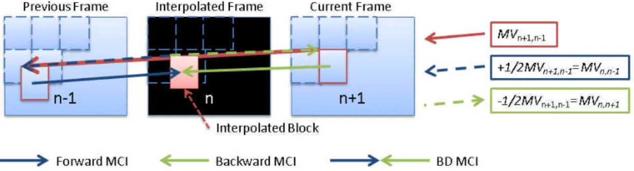
There have a lot of MCI models proposed for FRUC. Figure 2.1 shows three

different methods of MCI from the viewpoint of interpolation direction: forward MCI,

backward MCI and bi-directional MCI. In Figure 2.1, the MVn+1, n-1 is obtained after

using ME by block match algorithm from current frame to previous frame. The

forward MCI is taking the reference block as to-be-interpolated block along the half

forward motion vector (called MVn, n-2 in Figure 2.1) from previous frame. And the

backward MCI has the same concept as forward MCI, taking the reference block from

current frame along the half backward motion vector (called MVn, n+1 in Figure 2.1).

The bi-directional MCI considers both forward and backward motion vectors and gets

the averaging of two reference blocks as the to-be-interpolated block.

 

Figure 2.1 Non-alignment Motion Compensated Interpolation

 

5 

interpolated frame to have no or block artifacts such as a hole or an overlapped area

can occur on the interpolated frame. For this kind of the interpolation methods in MCI,

we call them “non-alignment MCI” in this paper because the block mapping to

interpolated frame may not have the same block position in the interpolated frame.

Figure 2.1 shows the non-alignment MCI.

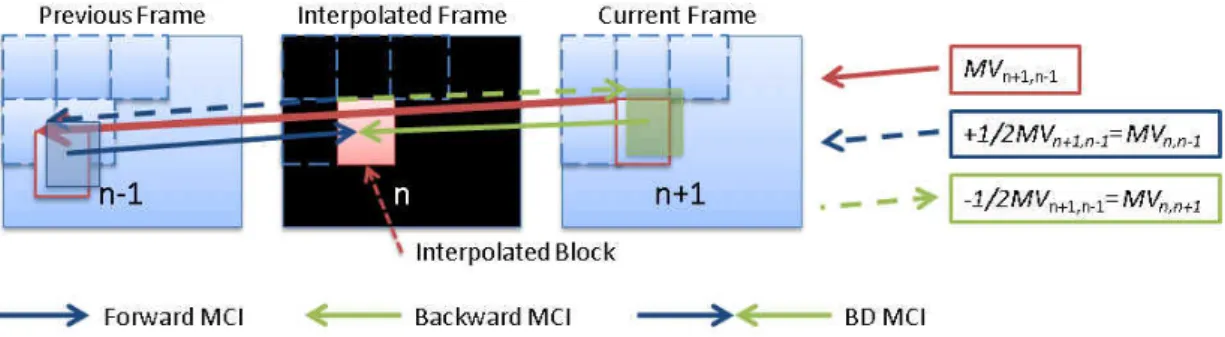
In contrast with non-alignment MCI, a number of researchers have proposed to

avoid the problems of holes and overlaps [1], [3]. These methods we call them

“alignment MCI” contrast to non-alignment MCI in this paper.

Figure 2.2 illustrates the MC-FRUC approach using bi-directional motion fields.

This approach divides the frame to be interpolated into blocks before it is actually

created. Each block has two motion vectors, one pointing to the previous frame and

the other to the next frame. The pixels in the block are interpolated by motion

compensation using these two motion vectors. The motion vectors are derived from

unidirectional motion estimation. The apparent advantage of the bi-direction approach

is that there is no need to handle holes and overlaps. But the MV which mapped to

interpolated frame is not real MV trajectory from current frame to previous frame.

 

Figure 2.2 Alignment Motion Compensated Interpolation

6 

video coding, the smaller block size produces a small amount of residual energy but

more computation. In contrast, the large block size obtains true MV for having higher

video quality. So whether it is in ME or MCI have a certain amount of computing cost.

Therefore, some research in MCI aim to reduce computation complexity and enhance

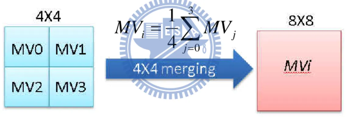
visual quality. In[4], [5], 8X8 block size is selected as basic processing unit to trade

off energy reduction of residual images and the correctness of obtained motion

vectors. For block large than 8X8, each constituent 8X8 block may have the same

motion vectors as that of original blocks. For block small than 8X8, it calculates the

average of the motion vectors of all its sub-blocks to be the new one. The Figure 2.3

shows, the MV after merging (i.e., MVi) is the average MV of 4 sub-MVs in block

4X4.

 

Figure 2.3 Average Motion Vector Merging

2.2 Spatial Interpolation Model

In [7], the spatial concealment utilizes the bilinear interpolation to conceal the

missing pixels. It reconstructs the missing pixels by averaging between adjacent

pixels. In Figure 2.4, to conceal the center missing pixel value, and the A, B, C, D,

and E neighboring pixels are all referenced. Equation 2.1 is the bilinear interpolation

algorithm for Figure 2.4.

Missing Pixel A

B

C

D

E 5

⁄ (2.1)

∑

=

=

3 0

4

1

j j i

MV

MV

7 

   

Figure 2.4 Neighbor pixel and missing pixel for Spatial interpolation

A non-linear interpolator, called edge sensing, is proposed for error concealment

in MDC application [7]. The edge sensing algorithm is based on gradient calculation

of the lost pixels. Figure 2.4 illustrates the center missing pixel is predicted by A, B, C

and D and two gradients will be calculated in horizontal and vertical directions. With

the two gradients, the more smooth direction can be determined, and averaging the

pixels in this direction has a better concealment effect than using a bilinear

interpolator.

2.3 Interpolation selection based on

gradient calculation

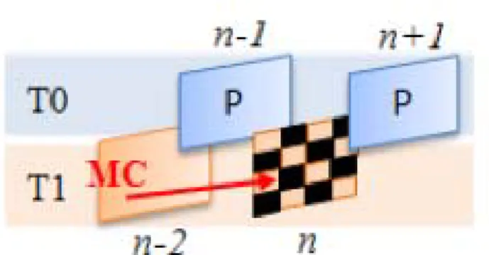
In [8], the interpolation selection utilizes the gradient calculation to conceal the

loss pixels in multiple description video coding (MDC). It segments video sequence

along spatial and temporal domain. Figure 2.5 shows the temporal segmentation

which splits the video into even and odd sub-sequences, called T0 and T1. Figure 2.6

shows the spatial segmentation which poly-phase permuted inside the block 8X8 and

then split to 2 blocks. The middle of Figure 2.6 shows the poly-phase permuting

results, then the splitting process is performed to split each 8X8 block into two 8X8

blocks, called R0 and R1. It produces 4 descriptions after video segmentation on

8 

 

Figure 2.5 Temporal Splitting in encoded side

 

Figure 2.6 Spatial Splitting in encoded side

 

Figure 2.7 Poly-phase inverse in decoded side

 

Figure 2.7 shows poly-phase inverse in decoded side when one description loss.

It can reconstruct loss pixel by bilinear interpolation as spatial interpolation (i.e.,

red-cross part in Figure 2.7) or motion compensated interpolation with previous frame

as temporal interpolation in the same description (i.e., MC from frame n-2 to n in

Figure 2.4). And it used spatial and temporal gradients to choose which interpolation

9 

,

_{, ,}

,

_{, ,}

(2.1)

where S, T denotes spatial and temporal interpolation, respectively. GSn(x, y)

and GTn(x, y) are spatial and temporal gradient of pixel (x, y) in frame n,

10 

Chapter 3 

Proposed Method

In this chapter, the relation between pixel gradients and visual quality is explored

using statistical approach first, then the mechanism of choosing interpolation methods

according pixel gradients is described, and finally, a FRUC method is proposed.

3.1 Exploring Relation Between Pixel

Gradient and Visual Quality

MC-FRUC methods typically exploit high correlation of motion information in

successive frames, namely, utilizing the relation in temporal domain. In addition to

temporal relation, the proposed FRUC method also exploits high relevance of the

adjacent pixels in the same frame, namely, utilizing the relation in spatial domain. To

determine which relation is more important to each individual pixel, pixel gradients

are used, as the error concealment method adopted in [7]. In this section, we first

propose how to measure pixel gradients in both temporal and spatial domains, and

then describe our observation on the relation between pixel gradients and visual

quality (i.e., Peak signal to noise ratio, PSNR) by using statistical method.

A non-linear interpolator, called edge sensing, is proposed for error concealment

in MDC application [7]. The edge sensing algorithm is based on gradient calculation

of the lost pixels. Figure 2.4 illustrates the center missing pixel is predicted by A, B, C

11 

the two gradients, the more smooth direction can be determined, and averaging the

pixels in this direction has a better concealment effect than using a bilinear

interpolator.

3.1.1 Pixel Gradient Measure

Instead of measuring pixel gradients as in [7] where the gradient is calculated by

horizontal and vertical directions, the more smooth direction can be determined, and

averaging the pixels in this direction. We consider six directions of pixel gradient in

spatial domain: horizontal direction (represented by the symbol “H”), vertical

direction (“V”), cross direction (“C”), 45-degree direction (“D1”), 135 degree

direction (“D2”) and cross of 45-degree and 135-degree directions (“D”), respectively.

Let the pixel in black denotes the to-be-interpolated pixel, Figure 3.1 illustrates the six

directions of pixel gradients for it.

 

Figure 3.1 6 type of spatial gradient for interpolated pixel

The pixel gradient (GP) in spatial domain is calculated as the average of the

difference between its two or more adjacent pixels in variable directions. Let Pn(i, j)

12 

this to-be-interpolated pixel at direction d is GPnd(i, j). The proposed six directions of pixel gradient are defined as:

, , ,

(3.1)

, , ,

(3.2)

, , , , ,

(3.3)

, , ,

(3.4)

, , ,

(3.5)

, , , , ,

(3.6)

 

In temporal domain, the motion compensated gradient (GMC) of a to-be-

interpolated pixel is measured as the difference between the motion-compensated

pixel in reference frame and the pixel at extrapolated location in the current frame. In

Figure 3.2, assume that the MV of each block in the to-be-interpolated frame (say

frame n) is the same to the MV of the co-located block in the current frame (i.e.,

frame n+1). The motion vector (i.e., MVn+1, n-1) from current frame to reference frame

(i.e., frame n-1) is divided into two, a forward MV denoted by (fx fy) which is defined

as +1/2MVn+1, n-1 and a backward MV denoted by (bx,by) which is defined as

-1/2MVn+1,n-1. The motion compensated temporal gradient of the to-be-interpolated

pixel is then defined as:

, , ,

(3.7)

13 

 

Figure 3.2 Temporal gradient of interpolated pixel

3.1.2 Gradient-PSNR relation

Intuitively, when the content of a video has the characteristics of simple textured

and high-motion, it is more appropriate to use spatial interpolation is. In contrast,

when the features of a video are slow-motion and complex textured, using temporal

interpolation would be better. In order to effectively choose appropriate interpolation

methods for above cases, we explore the relation between PSNR of different

interpolation methods and the gradient values by using statistical method. The

experiments were conducted for 2075 frames form 8 different QCIF sequences. All

frames are interpolated using the bi-direction MCI as temporal interpolation and six

different spatial interpolations from six different directions as proposed in previous

section. We calculate the average gradients per frame both in spatial and temporal

domains, which are denoted respectively as follows:

∑

∑

_,

(3.8)

∑

∑

_,

(3.9)

where GSn denotes the average spatial gradient of frame n, and GTn denotes the

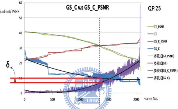
fram GT_ and Sim dire is d incr obse GS_ othe   me, respecti In Figure _PSNR. Th the averag milarly, the P ection is den denoted by reases, and erved that t _C_PSNR, er. Similar p In Figu PSNR and between th indicates th vely. 3.3, the PS he results of ge temporal PSNR of ea noted by G GS_C in F there is a si there is a si where on e phenomenon Figure 3. ure 3.4, by two gradie he two grad hat, by mo SNR of a fr f all frames gradient, G ach corresp GS_C_PSNR Figure 3.3. imilar trend ingle interse each side of n also happ .3 Relation using the ent curves, ient curves oving down 14  rame using s are sorted GT, of each onding fram R and the co As expect d between th ection for t f the interse ens on the t between gra quadratic p it is more on the inte n the GS_C temporal i d in a desce h correspon me using sp orrespondin ted, the GT he GS_C_P he two PSN ection, one two gradien adient value a polynomial clearly to ersection po C curve fo nterpolation ending orde nding frame patial interp ng average T_PSNR de PSNR and G NR curves, curve is alw nt curves, G and PSNR trend line

see the dif

oint of PSN or about δ n is denoted er of GT_PS e is also sho polation at c spatial grad ecreases as GS_C. It is GT_PSNR ways above T and GS_C to fit both fference (sa NR curves. units, the d by SNR own. cross dient GT also R and e the C.   two ay δ) This two

15 

intersection points will happen on the same frame. Then, almost all the frames

with GT lower than GS_C will have higher GT_PSNR than GS_C_PSNR,

indicating that temporal interpolation is preferred for these frames. On the other

hand, for those frames with GS_C lower than GT, spatial interpolation is preferred

because a higher PSNR can be obtained.

 

Figure 3.4 Differential value (delta) of spatiotemporal-gradient

 

 

16 

In Figure 3.5, there are 6 spatial gradient and PSNR curves obtained from spatial interpolation in 6 different directions, each of them have different delta value (i.e., δH,

δV,  δC, …), where only δC for cross direction is shown. The result in Figure 3.5 also

indicates that the priority of spatial interpolation directions can be determined

according to the position of intersections of PSNR curves. The GS_C_PSNR has first

intersection with GT_PSNR, and then is GS_H_PSNR, GS_V_PSNR, GS_D_PSNR,

GS_D2_PSNR, and GS_D1_PSNR, indicating that priorities of spatial interpolations

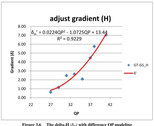
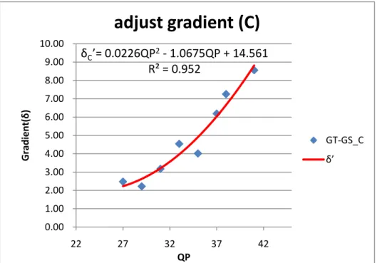
are C, H, V, D, D2 and D1. By conducting more experiments with more QPs, we found that δ is a function of QP. As depicted in Figure 3.6 to 3.11 where 8 different

QPs ranging from 27 to 41 in 6 directions are used, the relation between δ and QP can

be modeled using q quadratic equation as follows.

0.0224

1.0725

13.44 3.10

0.0044

0.147

6.4262 3.11

0.0226

1.0675

14.561 3.12

0.0301

1.2912

11.891 3.13

0.0106

0.0927

5.1688 3.14

0.0303

1.3125

13.35 3.15

17 

 

Figure 3.6 The delta-H (δH) with difference QP modeling

 

Figure 3.7 The delta-V (δV) with difference QP modeling

δ_H’ = 0.0224QP2_{‐ 1.0725QP + 13.44} R² = 0.9229 0.00  1.00  2.00  3.00  4.00  5.00  6.00  7.00  8.00  22 27 32 37 42 Gradient  ( δ ) QP

adjust gradient (H)

GT‐GS_H δ’ δ_V’ = 0.0044QP2_{+ 0.147QP ‐ 6.4262} R² = 0.9105 0.00  1.00  2.00  3.00  4.00  5.00  6.00  7.00  8.00  22 27 32 37 42 Gradient( δ ) QP

adjust gradient (V)

GT‐GS_V δ’

18 

   

Figure 3.8 The delta-C (δC) with difference QP modeling

   

Figure 3.9 The delta-D1 (δD1) with difference QP modeling

δ_C’= 0.0226QP2_{‐ 1.0675QP + 14.561} R² = 0.952 0.00  1.00  2.00  3.00  4.00  5.00  6.00  7.00  8.00  9.00  10.00  22 27 32 37 42 Gradient( δ ) QP

adjust gradient (C)

GT‐GS_C δ’ δ_D1’ = 0.0301QP2_{‐ 1.2912QP + 11.891} R² = 0.9407 ‐2.00  0.00  2.00  4.00  6.00  8.00  10.00  12.00  22 27 32 37 42 Gradient( δ ) QP

adjust gradient (D1)

GT‐GS_D1 δ’

19 

   

Figure 3.10 The delta-D2 (δD2) with difference QP modeling

   

Figure 3.11 The delta-D (δD) with difference QP modeling

Then, for each unreliable pixel, adjust its six spatial gradients (i.e., GSH, GSV,

GSC, GSD1, GSD2, and GSD) by using their corresponding delta values, , , ,

, , and , respectively. These delta values are predefined by statistic

method as described in Section 3.1. Let denote the GSx after adjustment by

δ_D2’ = 0.0106QP2_{‐ 0.0972QP ‐ 5.1688} R² = 0.8609 0.00  1.00  2.00  3.00  4.00  5.00  6.00  7.00  8.00  9.00  10.00  22 27 32 37 42 Gradient( δ ) QP

adjust gradient (D2)

GT‐GS_D2 δ’ δ_D’ = 0.0303x2_{‐ 1.3125x + 13.35} R² = 0.9308 0.00  2.00  4.00  6.00  8.00  10.00  12.00  22 27 32 37 42 Gradient( δ ) QP

adjust gradient (D)

GT‐GS_D δ’

20 

, i.e., , and ITPx denote interpolation method x, where x can be

H, V, C, D1, D2, or D. Then, the spatial interpolation method, ITPx, will be used

for an unreliable pixel Punreliable if the neighbor pixels required for interpolation

method x are all reliable and the equation 3.16 below is hold.

ITP

P

unreliable , 3.16

As an example in Figure 3.12, assuming that the center pixel in black is the

unreliable pixel to be interpolated, then it will be interpolated by ITPH only when its

left and right neighboring pixels are both reliable and . Similarly, it will be

interpolated by ITPD only when its right-up, right-down, left-up, and left-down

neighbor pixels are all available and . When multiple spatial interpolation

methods meet the conditions, the interpolation method is selected according to the

priority determined by Fig.3.5 as described in Section 3.1, where the interpolation

priorities from high to low are ITPC, ITPH, IPTV, ITPD, ITPD2, and ITPD1 ,

respectively.

 

Figure 3.12 selection of spatial interpolation type

21   

3.2 Proposed FRUC algorithm

The proposed FRUC method aims at doubling frame rate, namely, converts the

frame rate from n to 2n. Figure 3.13 shows the concept, where suppose that the

input sequence will become even frames of the up-converted sequence and we need to

produce all odd frames by the proposed method. We call these non-existing odd

frames as the to-be-interpolated frames.

Figure 3.13 Frame rate up-conversion from n to 2n

 

The proposed FRUC algorithm is summarized with following flow chart in

Figure 3.14. The proposed algorithm mainly divided into two parts. The first part

including steps 1, 2, and 3 is frame-based temporal interpolation to generate the initial

interpolated frame. The second part including step4 is pixel-based spatial

interpolation to improve visual quality with various non-linear interpolation methods

by pixel gradients determination. The detail of each step will be described in the

22 

 

Figure 3.14 Flow chart of proposed FRUC algorithm

23   

3.2.1 ME & Motion Vector Merging

Step1 of the proposed method includes a block-based unidirectional motion

estimation process which is applied to every adjacent frame of the input sequence by

using block matching algorithm for obtaining the best motion vectors for each block

as the Fig.3.15 shows.

 

Figure 3.15 Motion Estimation in proposed method

 

Step 2 of the proposed method includes a MV merging process. In the video

coding standard H.264, block sizes vary from 16x16 to 4x4. In our approach, for any

block which is smaller than 8x8, it will be merged with its neighbor blocks into an

8x8 block. The MV of the merged 8x8 block is chosen as the median of the motion

vectors of all its sub-blocks. Since the median MV should have minimal distances

between it and other three MVs, our median function is defined as: the median MV is

the one which has the minimum SAD (sum of absolute difference) between it and the

other three neighboring MVs. This is different from traditional MV merging which

adopts average MV as the merged MV. The Figure 3.16 shows an example of our MV

merging, where there are 4 neighboring 4x4 sub-blocks. Use the proposed median

function to determine the median one among the four motion vectors, MV0 ~ MV3. If

MVi is selected, then it will become the MV of the resulting 8x8 block. MV merging

processing not only can reduce MCI computation (because number of MVs is

24 

experimental results.

Figure 3.16 MV merging by median selection 

3.2.2 Temporal Interpolation model

In the step3 of the proposed algorithm, the initial interpolated frame is generated

by two bi-directional MCI methods. The non-aligned bi-directional MCI

(NA-BDMCI) is performed first, which produces interpolated pixels by averaging the

pixels on the adjacent frames along real motion trajectory. The real motion trajectory

is derived from the motion vectors of adjacent frames, obtained by motion estimation

process in step1. The NA-BDMCI is illustrated as the Fig.3.17 shows.

Figure 3.17 non-aligned bi-directional MCI (NA-BDMCI)

After NA-BDMCI, there may have some holes on the interpolated frame, due to

no motion trajectory on them. Thus, a aligned bi-directional MCI (A-BDMCI) is

)

(

_=0~3

=

_j

i

median

MV

25 

performed to overcome this problem. Different from NA-BDMCI which uses real

motion trajectory, A-BDMIC uses motion vectors of the co-located blocks on adjacent

frames as the motion vectors of the interpolated frame and thus, every aligned block

in the interpolated frame will have a motion vector. In our approach A-BDMIC is only

used to produce the pixels on the hole of the interpolated frame generated by

NA-BDMCI. The A-BDMCI is illustrated as the Fig.3.18 shows.

Figure 3.18 aligned bi-directional MCI (A-BDMCI)

Producing pixels by using BDMCI methods typically has the pixel overlapping

problem, that is, multiple pixels are interpolated corresponding to the same location.

There are two alternatives to be used in common: average selection and minimum

absolute difference (MAD) selection. The average selection uses the average pixel

value of all the overlapped pixels; while the MAD selection chooses the pixel value

from the one which has minimum absolute difference between the motion

compensated pixels on the two adjacent frames. In our solution, average method is

26 

3.2.3 Spatial Interpolation model

In the step4 of the proposed algorithm, a pixel-based spatial interpolation is

adopted. The flow chart is shown in Figure 3.19.

 

Figure 3.19 Flow chart of pixel-based spatial interpolation model

 

First, it calculates the gradients both in temporal and spatial (containing 6

different directions) domains for each pixel on the initial interpolated frame produced

by step3. Second, it distinguishes reliable and unreliable pixels according to temporal

gradient threshold (GT_TH) which is a value predefined by using statistic method.

For those pixels identified to be unreliable, they will be modified by using spatial

interpolation method because their initial values produced by temporal method are not

27 

Figure 3.20 shows how the threshold value of GT is defined. It is obtained by

using temporal interpolation and spatial interpolation respectively on all the pixels of

each frame for eight training sequences. The corresponding PSNR values and gradient

values (both in frame-based) are presented in the ascending order of PSNR value of

spatial interpolation and the descending order of PSNR value of temporal

interpolation. From Fig.3.20, it is observed that on the left side of the intersection of

two PSNR curves, the temporal interpolation has better results than spatial

interpolation. So the frames with temporal gradients (GT) falling in this region are

regarded to be reliable if temporal interpolation is used. Hence, we use the average of

GTs in this region as the GT_TH and use the equation (3.17) to determine whether a

pixel, p, at location (x, y) of frame n is reliable or not, where ‘1’ means the pixel is

reliable and ‘0’ means unreliable.

,

1,

_,

_

0,

(3.17)

 

28 

Chapter 4 

Experimental Results

To examine the performance of proposed methods, we use four test video

sequences with QCIF (176x144) resolution and split those test sequences into two

subsequences; one consisting of all odd frames and the other all even frames. Then,

we get reconstructed even frames by encoding the even sequence with H.264/AVC

reference software, JM 16.0 [9], and perform the proposed FRUC algorithm on the

reconstructed even frames to generate all odd frames. The performance is then

evaluated by comparing the interpolated odd frames with original odd frames. The

proposed methods are compared with MCI method for both objective and subjective

visual qualities. The objective quality is measured using Peak Signal-to-Noise Ratio

(PSNR) which is defined by Equation (4.1)

10

4.1

, where

∑ ∑ _{, ,}

4.2

, where height and width are the frame resolution in vertical and horizontal directions,

respectively; _, is the pixel value of the original sequence and _, is the pixel value

generated (or interpolated) by the decoder.

4.1 Environments & Model Parameters

29 

¾ Frame Rate: 30

¾ Encoded frames :125~300

¾ Training sequence: 8 sequences

¾ Test sequence: 4 sequences

Table 4.1 lists the test and training sequences used in our experiments. The eight

training sequences are used for determining temporal gradient threshold GT_TH and

the ’ in six directions. For test sequences, we take their reconstructed even frames

(i.e., 150 frames) as the input of our FRUC algorithm for producing odd frames.

training seq.  8  test seq.  4 

Frame No.   

training seq.  whole seq. half seq. (even) 

akiyo  300  150  container  300  150  hall  300  150  carphone  300  150  silent  300  150  stefan  300  150  football  125  62  soccer  150  75  test seq.      mobile  300  150  foreman  300  150  coastguard  300  150  news  300  150   

Table 4.1 Test sequences and training sequences

 

Three proposed methods as well as the conventional bi-directional MCI method

30 

For all methods, they have common process in step 1 for obtaining motion vectors by

motion estimation. For steps 2 to 4, different methods adopt different schemes as

listed in Table 4.2 below. As the table shows, MCI algorithm adopt average selection

for MV merging [4], deals with hole-region problem in [3] and MAD strategy for

solving pixel overlapping problem. Spatial interpolation is not used in the MCI

method. Compared with MCI, our proposed_1 method simply changes the MV

merging strategy in step2 by using median selection. Compared with proposed_1, the

proposed_2 solves the pixel overlapping problem in step 3 by using average instead of

MAD strategy. Compared with proposed_2, the proposed_3 method adds pixel-based

spatial interpolation in step4 for unreliable pixels.

 

Table 4.2 Four methods adopted for comparison.

 

4.2 Performance of Objective Quality

In this section, experimental result of objective quality is presented. Figure 4.1

depicted the average PSNR (dB) values of interpolated frames as a function of QPs

for four sequences: (a) mobile, (b) foreman, (c) coastguard and (d) news sequences. It

is clearly seen that all proposed methods perform better than MCI for 4 test sequences.

As expected, PSNR values decrease as the QP increases for all methods. Each of

proposed methods compared to MCI has average gains of 0.11dB, 0.16dB and 1.06

31 

proposed_2 and Proposed_3. The proposed_1 outperforms MCI method is due to that

the median selection used for MV merging is better than average selection. The result

of proposed_2 is close to proposed_1 (average gain 0.05dB), meaning that it makes

no much difference by using average or MAD in solving pixel overlapping problem.

Among all methods, proposed_3 has the best performance, indicating that the

proposed pixel-based spatial interpolation did perform well in improving the

performance produced by temporal interpolation. Since proposed_3 replaces the

unreliable pixels with interpolated neighboring pixels, the resulting frames are much

smother (with less blocking effects) than those using temporal interpolation only.

(a) 21.00  22.00  23.00  24.00  25.00  26.00  27.00  20 25 30 35 40 45 PSNR QP

mobile

MCI proposed_1 proposed_2 proposed_3

32  (b)     (c) 26.00  27.00  28.00  29.00  30.00  31.00  32.00  33.00  20 25 30 35 40 45 PSNR QP

foreman

MCI proposed_1 proposed_2 proposed_3 25 26 27 28 29 30 31 32 33 34 20 25 30 35 40 45 PSNR QP

coastguard

MCI proposed_1 proposed_2 proposed_3

33 

   

(d) 

Figure 4.1 PSNR of four sequences at Different QP. (a) Mobile. (b) Foreman. (c) Coastguard. (d)news

         

Table 4.3 gives the average PSNR of 5 test sequences at different QPs using MCI

and proposed FRUC algorithms. The values on the row of Gain denote the PSNR

gains of the proposed methods over MCI method.

 

Table 4.3 avg. PSNR of five sequences at different QP in MCI and proposed FRUC methods 26 27 28 29 30 31 32 33 34 20 25 30 35 40 45 PSNR QP

news

MCI proposed_1 proposed_2 proposed_3

34 

Figure 4.2 shows the frame-by-frame PSNR of (a) mobile and (b) foreman at

QP28. It is clearly seen that the proposed_3 yields an overall better performance than

the other three methods both in mobile and foreman sequence. The proposed_2 has

similar result with proposed_1, meaning that selecting MAD or average strategy for

solving pixel overlapping did not have much effect on the result.

   

(a)

   

(b) 

Figure 4.2 PSNR per frame of two sequences at QP28. (a) Mobile. (b) Foreman.

    21 22 23 24 25 26 27 28 29 0 10 20 30 40 50 PSNR Frame No.

Mobile @QP28

MCI proposed_1 proposed_2 proposed_3 25.5 27.5 29.5 31.5 33.5 35.5 0 10 20 30 40 50 PSNR Frame No.

Foreman @QP28

MCI proposed_1 proposed_2 proposed_3

35   

4.3 Spatial Interpolation ratio

In Fig.4.3, the percentage of the pixels interpolated by using spatial methods is

presented. It is observed that the percentage of spatial interpolation is decreased as the

QP increases. This holds for mobile, foreman and coastguard sequence. As for the

static sequence (with low-motion content), News, since its GT values are small, there

are only few unreliable pixels that will be used for spatial interpolation, resulting in

relatively low percentage.

 

Figure 4.3 Total percentage of spatial interpolation at difference QP in four sequences

 

In Figure 4.4 (a)-(d), the percentages of “H”, “V”, “D1” and “D2” conform to the

spatial interpolation priority. The type of spatial interpolation of “C” and “D” did not

follow the priority because the number of reliable neighboring pixels required for “C”

and “D” are more than the other four types, resulting much less percentage in type “C”

and type “D”, compared with other interpolation types.

0.00  1.00  2.00  3.00  4.00  5.00  6.00  7.00  8.00  24 28 32 36 40 % QP

Spacial Interpolation

mobile foreman coastguard news

36      (a)     (b) 0.00  0.20  0.40  0.60  0.80  1.00  1.20  1.40  1.60  1.80  2.00  24 28 32 36 40 % QP

mobile

Cross V H D D1 D2 total 5.42 5.00 3.21 3.37 3.18 0.00  0.20  0.40  0.60  0.80  1.00  1.20  1.40  1.60  24 28 32 36 40 % QP

foreman

Cross V H D D1 D2 total 4.88 3.77 3.23 3.84 3.85

37 

   

(c)

   

(d)

Figure 4.4 The percentage of 6 type spatial interpolation at difference QP in four sequences (a) Mobile. (b) Foreman. (c)coastguard. (d)news.

    0.00  0.50  1.00  1.50  2.00  2.50  24 28 32 36 40 % QP

coastguard

Cross V H D D1 D2 total 7.05 5.39 3.23 3.23 2.48 0.00  0.05  0.10  0.15  0.20  0.25  0.30  0.35  0.40  0.45  0.50  24 28 32 36 40 % QP

news

Cross V H D D1 D2 total 1.41 1.16 1.06 1.19 1.13

38   

4.4 Performance of Subjective Quality

 

Figure 4.5 (a)-(d) shows the images interpolated by using MCI, proposed_1,

proposed_2, and proposed_3, respectively. It can be seen that the images from MCI

and proposed_2 show obvious blocking artifacts around cap edge and the hypotenuse

of background buildings. Compared with MCI and proposed_1, the image by using

proposed_2 shows a little improvement on visual quality. Among all images, the one

produced by proposed_3 shows the best visual quality with neglect able blocking

artifacts.

(a) (b)

   

(c) (d)

Figure 4.5 Interpolated results of frame 18 of Foreman sequence at QP28 using

(a) MCI. (b) proposed_1. (c) proposed_2. (d) proposed_3.

 

39 

Chapter 5 

Conclusion

A frame rate up-conversion based on temporal and spatial interpolation had been

proposed. The temporal interpolation is a frame-based interpolation which combined

two MCI methods, one is non-aligned bi-directional MCI (NA-BDMCI) for real

motion concealment on to-be-interpolated frame, and the other is aligned A-BDMCI

for overcoming the hole-region problem. The proposed spatial interpolation is a

pixel-based non-linear interpolation method which considers the relationship between

PSNR and spatiotemporal gradient to interpolate unreliable pixels for improving

visual quality.

According to the experimental results, it is observed that, using median selection

in MV merging is more effective than using average selection. Besides, with the

average selection on solving pixel overlapping, there is only a little enhancement to

the quality of image; and with spatial interpolation, there is a significant improvement

40 

Reference

[1] T. Chen, "Adaptive temporal interpolation using bidirectional motion estimation

and compensation", IEEE International Conference of Image Processing 2002,

pp. 313-316.

[2] K. Hilman. H. W. Park, and Y. Kim, "Using motion-compensated frame-rate

conversion for the correction of 3:2 pulldown artifacts in video sequences," IEEE

Trans. Ciruits Syst. Video Technol., vol. 10, no. 6, pp. 869-877, Sept. 2000.

[3] B.-T. Choi, S.-H. Lee, and S.-J. Ko, “New frame rate up-conversion using

bi-directional motion estimation,” IEEE Trans. on Consumer Electronics, Aug.

2000, Vol. 46, No. 3, pp. 603-609.

[4] J. Zhai, K. Yu, J. Li, and S. Li, “A low complexity motion compensated frame

interpolation method,” in Proc. IEEE SCAS, May 2005,pp. 23–26.

[5] Y.-T. Yang , Y.-S. Tung and J.-L. Wu "Quality enhancement of frame rate

up-converted video by adaptive frame skip and reliable motion extraction", IEEE Trans. Circuit Syst. Video Technol., vol. 17, p.1700 , 2007.

[6] D. Wang "Motion-compensated frame rate conversionPart II: New algorithms

for frame interpolation", IEEE Trans. Broadcasting, vol. 56, , 2010.

[7] R. Bemardini, M. Durigon, R. Rinaldo, L. Celetto, and A. Vitali, “Polyphase

Spatial Subsampling Multiple Description Coding of Video Streams with H.264,”

Proceedings of IEEE International Conference on Image Processing(ICIP), 2004.

[8] J.-Y Chen, W.-J. Tsai, “Joint temporal and spatial multiple description coding for

H.264 video,” Proceedings of IEEE International Conference on Image

Processing (ICIP), 2010, pp. 1273-1276.